Other uses, including reproduction and distribution, or selling or licensing copies, or posting to personal, institutional or third party
websites are prohibited.
In most cases authors are permitted to post their version of the article (e.g. in Word or Tex form) to their personal website or institutional repository. Authors requiring further information
regarding Elsevier’s archiving and manuscript policies are encouraged to visit:
Mechanical Systems
and
Signal Processing
Mechanical Systems and Signal Processing 22 (2008) 1374–1394On the HHT, its problems, and some solutions
R.T. Rato, M.D. Ortigueira
,1, A.G. Batista
Campus da FCT da UNL, Quinta da Torre, 2825 - 114 Monte da Caparica, Portugal
Received 15 December 2006; accepted 30 November 2007 Available online 18 January 2008
Abstract
The empirical mode decomposition (EMD) is reviewed and some questions related to its effective performance are discussed. Its interpretation in terms of AM/FM modulation is done. Solutions for its drawbacks are proposed. Numerical simulations are carried out to empirically evaluate the proposed modified EMD.
r2007 Elsevier Ltd. All rights reserved.
Keywords:Empirical mode decomposition; Intrinsic mode function; Parabolic interpolation; Extrema detection; Amplitude–frequency modulation
1. Introduction
The empirical mode decomposition (EMD) [1] is a technique to decompose a given signal into a set of elemental signals called ‘‘intrinsic mode functions’’ (IMFs). The EMD is the base of the so-called ‘‘Hilbert–Huang transform (HHT)’’ [1] that comprises the EMD and the Hilbert spectral analysis that performs a spectral analysis using the Hilbert transform (HT) followed by an instantaneous frequency computation.
The algorithm is simple and gives good results in situations where other methods fail. However, it has some drawbacks, tied with some of the assumptions needed to implement the algorithm, leading to unexpected results. There have been several attempts to solve such problems. For example, Rilling et al.[2,3]made some algorithmic variations and proposed a new stopping criterion. Besides, they gave an interpretation in terms of filter banks. They also studied the influence of sampling[4]. On the other hand, Junsheng et al.[5]studied the behaviour of the decomposition algorithm and proposed an energy difference tracking method to define a coherent stopping criterion. In another attempt [6]they use the Teager–Kaiser [7]energy operator to extract the amplitude and instantaneous frequency of a multi-component amplitude-modulated and frequency-modulated (AM/FM) signals. The problem of envelope estimation is considered by Qin and Zhong who proposed the segment power function method [8].
In this paper, we make a global appreciation of the different aspects of the algorithm, considering its drawbacks and suggesting modifications to alleviate such problems. The most important is the extrema
www.elsevier.com/locate/jnlabr/ymssp
0888-3270/$ - see front matterr2007 Elsevier Ltd. All rights reserved. doi:10.1016/j.ymssp.2007.11.028
Corresponding author. Tel.: +351 1 2948520; fax: +351 1 2957786.
E-mail addresses:rtr@uninova.pt (R.T. Rato),mdo@fct.unl.pt (M.D. Ortigueira),agb@fct.unl.pt (A.G. Batista). 1
determination by using a parabolic approximation and the instantaneous amplitude and frequency computation that we propose to be done through an amplitude demodulation and first-order autoregressive (AR) approximation[9,10].
The paper outline is as follows. In Section 2 we describe the EMD algorithm as proposed in[1]and look inside it to understand the main difficulties and ways of avoiding them. In Section 3 we present the proposed solutions to such problems. In Section 4, we present some examples to illustrate the behaviour of the algorithm and to understand its features. Finally, we present some conclusions.
2. The EMD
2.1. Outline of the EMD algorithm
The EMD as proposed by Huang et al. [1] is a signal decomposition algorithm based on a successive removal of elemental signals: the IMFs. Given any signal,xðtÞ, the IMFs are found by an iterative procedure called sifting algorithm, which is composed of the following steps:
(a) Find all the local maxima, Mi;i ¼1;2;. . .; and minima, mk, k¼1, 2;. . .;in xðtÞ.
(b) Compute the corresponding interpolating signals MðtÞ:¼f
MðMi;tÞ, andmðtÞ:¼f
mðmk;tÞ. These signals are the upper and lower envelopes of the signal.
(c) Let eðtÞ:¼ðMðtÞ þmðtÞÞ=2.
(d) Subtract eðtÞ from the signal:xðtÞ:¼xðtÞ eðtÞ.
(e) Return to step (a)—stop when xðtÞremains nearly unchanged.
(f) Once we obtain an IMF,jðtÞ, remove it from the signalxðtÞ:¼xðtÞ jðtÞand return to (a) ifxðtÞhas more
than one extremum (neither a constant nor a trend).
The interpolating function is a cubic spline. By construction, the number of extrema should decrease when going from one IMF to the next, and the whole decomposition is expected to be completed with a finite number of IMFs (see [2]). We must remark that, at least conceptually, the algorithm:
is simple; appears naturally; does not assume anything about the signal, mainly stationarity; can be applied to a wide class of signals.2.2. The EMD as an AM/FM decomposition
Consider the sifting process. The first step finds two sets of points that constitute samples of two discrete-time signals. The interpolated signals give estimates of the upper and lower envelopes. If the envelopes were symmetric we would say thatxðtÞis an AM signal [11]. The sifting procedure is an iterative way of removing the dissymmetry between the upper and lower envelopes in order to transform the original signal into an AM signal. At least conceptually, this goal would be achieved in a few steps if:
The extrema were correctly determined. We had no problems with the interpolation at the extremities. We had no computational errors.These difficulties will be considered later.
In spectral terms, we can say that the bandwidth of the envelopes must be a fraction of the central frequency of
xðtÞ(normally called carrier). This means that when performing the sifting we are removing the low frequency components. So, we are leaving a high frequency signal. This explains why the IMFs appear in a high to low frequency order and why the EMD is essentially a time-frequency decomposition. This also explains why the EMD behaves like a bank of filters[3]. This also explains an interesting phenomenon: if we add two IMFs with non-intercepting bands, they will be decomposed without great distortion, but if the bands intercept, they will be decomposed into a set of several IMFs. We will show this later.
2.3. On the IMF
For the continuous case, an abstract IMF is defined as a signal that satisfies two conditions[1]:
In the whole signal segment, the number of extrema and the number of zero crossings must be either equal or differ at most by one. At any point, the mean value of the envelope defined by the local maxima and the envelope defined by the local minima is zero.This is the original definition of IMF presented in [1]. However, the first condition is redundant unless the function at hand is discontinuous. In fact, if a function verifies the second condition, it verifies the first also, because between a peak and a valley there is always a zero, since the envelopes are symmetric.
It is not difficult to see that sinusoidal signals sinð2pftÞor cosð2pftÞfor any realf and tare IMFs. It is not difficult to recognize that if FðtÞ is a continuous function, the same happens with sin½FðtÞ and cos½FðtÞ. These are well-known functions in telecommunications where they are studied under the name of ‘‘angle modulation’’ [11]. The instantaneous frequency is, aside a constant, the derivative of FðtÞ. Now, let us consider a function gðtÞ ¼AðtÞsin½FðtÞ. This is what is called ‘‘double side band’’ modulated sinusoid. In general, it is not an IMF, even if AðtÞ is also a sinusoid. But, if AðtÞ changes slowly when compared with the changes in sin½jðtÞ, we have really an IMF. So, we can say that a function of the typeAðtÞsin½FðtÞ
represents an IMF, provided thatAðtÞis a slowly varying function. This is the so-called envelope. But we must remark that the above definition of envelope may not be a true envelope. A simple example shows this. The functionxðtÞ ¼ejtjsinð2pftÞ has ejtj as envelope, but almost all the extrema points ofxðtÞ do not belong to
ejtj. In some signals this fact has as consequence that the function may have segments above (below) the envelope defined by the maxima (minima). As a conjecture, we can say that the extrema envelope coincides with the ‘‘true’’ envelope when this has extrema locations equal to those of the signal. However, there is no simple way of defining the ‘‘true’’ envelope and the extrema defining envelope seems to be suitable to our objectives.
We can conclude that the definition of IMF is tied with the definition of envelope that depends also on the interpolating function used to estimate it. So, the Huang et al. [1] IMFs correspond to the cubic spline interpolator. With other interpolator we may obtain a different set of IMFs. In our simulations we also used the Akima interpolator.2 The results were very similar.
2.4. Main drawbacks of the EMD
Let us take a look into the above described algorithm and consider the most important steps:
extrema locations; extrema interpolation; end effects; sifting stopping criterion; IMF removal.2
As we have seen in the earlier last sections, the algorithm has some implicit difficulties and the procedures used in previous papers[1–3]for the above steps create several drawbacks that originate ‘‘strange’’ decompositions. For example, when trying to decompose a sinusoidal segment, it is expected to obtain only one IMF and no residual. This may not happen with the available algorithm implementations[1–3].
We are going to look into each step and see why it creates difficulties. We begin by the extrema computation. This does not have an obvious solution. Although most data are originated by continuous-time processes, in practice, the algorithm operates on quantized discrete-time signals. When working with this kind of signals, some special attention is necessary because the extrema may not be correctly identified. Most, if not all, of the continuous waveform actual extrema will fall in between sampling instants and will not be correctly localized. To avoid this difficulty, Rilling et al.[2]proposed the use of a fair amount of oversampling.
We have considered before the interpolation problem and the interpolation function choice. However, even if we made a reasonable choice, the effectiveness of the approximation is highly dependent on the extrema computation and may lead to some undesirable results. One of them is the ‘‘overshoots’’: the signal crosses the envelope. This affects the IMF estimation.
The end effects appear when we have to decide what to do with the first and last samples. The solution will affect the final decomposition:
To consider them as maxima and minima simultaneously (this forces all the IMFs to be zero at those points). To consider them as maxima or minima according to the nearest extremum in order to guarantee the alternation between maxima and minima. To leave them free[1].The stopping criterion is another source of problems due to its degree of arbitrariness, since it may not guarantee a total signal removal to obtain a ‘‘true’’ IMF.
According to the above description, the final step is the removal of the IMF from the signal. However, if the IMF is not well computed, we may be ‘‘adding’’ to the remaining signal a component that will appear in the following IMF. This explains partially why we do not obtain only one IMF in the case of a pure sinusoid.
3. Some attempts to obtain a better algorithm
3.1. A framework for modifying the algorithm
The EMD does not have an analytical formulation: it is based on a computational algorithm. So it performs according to its implementation details. When the same signal is fed into different EMD implementations, different results are obtained, as we will see in Section 5.1. This is confusing and inadequate. To achieve consistency and to be able to compare results, different implementations should be equivalent. Our goal is to establish a framework for EMD implementation to avoid the referred drawbacks (Section 2.4).
Based on this rationale, we state the following guiding principles to be followed in the design, implementation and checking of EMD programs:
The IMF set obtained by multiplying a constant value to all the samples in the signal should be the IMF set of the original signal multiplied by the same constant. Changing the mean of the signal, it should only change the trend related IMF (the last one), leaving all the others unchanged. The EMD of an IMF should be the IMF itself. The IMF set obtained from a time reversed signal should be the time reversed IMF set of the original signal.33
These rules suggest us to:
Remove the mean. Normalize the signal to a unit power.This last procedure is important when dealing with signals with very low amplitudes as in the case of biomedical signals.
3.2. The proposed solutions
3.2.1. The extrema locations
In practice, the algorithm operates on discrete-time signals. This deserves some special attention because the extrema definition cannot be based on a continuous neighbourhood, as in calculus. It is necessary to define a classificatory function to assert whether a given sample is, or is not, an extremum. The classification of a sample as an extremum must be based on the relation of the actual sample and its left and right neighbours. Except for the first and last samples, all samples vicinity will have just those two values. Larger vicinities, with more than two values, will distress the algorithm’s local feature. So, the classificatory function must receive as input just these three values. According to principle (d), commuting the preceding sample with the subsequent sample should not change a sample classification. A classification based solely on ‘‘4’’ and ‘‘X’’ type relations will adhere naturally to principles (b) and (c) seen in the previous section. For a given sample, x½n, the used classificatory function is
If ððx½n4x½n1ÞAND ðx½nXx½nþ1ÞÞ
ORððx½nXx½n1Þ AND ðx½n4x½nþ1ÞÞ Then Return (‘‘Is a Maximum’’)
Else if ððx½nox½n1ÞAND ðx½npx½nþ1ÞÞ
ORððx½npx½n1Þ AND ðx½nox½nþ1ÞÞ Then Return (‘‘Is a Minimum’’) Else Return (‘‘Not an extrema’’);
However, the envelope fitting depends on the extrema accuracy (position and value). As referred above, dealing with a discrete-time signal produces an error in the location of an extremum that can be equal to half the sampling interval. To alleviate this problem, we interpolate the signal in the interval defined by the two neighbours to obtain a better extremum location and individualization [4]. Classic interpolation for band limited signals relies on the computationally demanding sinc function as the interpolation kernel. This has the disadvantage of needing a lot of samples on the right and on the left.
In agreement with our comments in Section 2.3, we are expecting that the IMFs have some degree of smoothness, mainly near the extrema. In particular, they may also have a null derivative at the extrema. This means that, near the extrema, it can be approximated by a parabola. So, parabolic interpolation comes into sight as a practical compromise between no interpolations at all and sinc based interpolations, for better location of the extrema values. Using parabolic interpolation, each extremum is estimated from only the above defined three samples. A new interpolated extremum sample is obtained, usually with no integer abscissa, and this new sample is fed into the EMD algorithm, replacing the integer abscissa extremum sample as an envelope defining point. To see what happens, assume the situation where we have an extremum near timet¼n, and let
yð1Þ ¼x½n1, yð2Þ ¼x½n, and yð3Þ ¼x½nþ1. The interpolating parabola is defined by yðkÞ ¼ak2þb
kþc ðk¼1;2;3Þ. We have
yð1Þ
yð2Þ
yð3Þ
2 6 4 3 7 5¼
1 1 1 4 2 1 9 3 1
2 6 4 3 7 5 a b c 2 6 4 3 7 5 and a b c 2 6 4 3 7 5¼
1=2 1 1=2
5=2 4 3=2 3 3 1
2 6 4 3 7 5
yð1Þ
yð2Þ
yð3Þ
2
6 4
3
7
5. (1)
the extremum obtained from the interpolating parabola will be
tp¼
b
2a; yp ¼ b
2tpþc. (2)
If 1:5otpo2:5, we will have an extremum with a true location point att¼n2þtp; otherwise, there will not
be an extremum.
As simple reasoning shows, this procedure gets round the use of the above classificatory function. In fact, we can run the interpolation algorithm just described for all the tripletsx½n1,x½n, andx½nþ1formed with the samples of the signal. The first and last samples were not considered, leaving them as not extrema. This option was taken according to the procedure described in the next section.
3.2.2. The end effects
In Section 2.4 we referred the end effects. These appear due to the fact that a given interpolator may not be a good extrapolator (see Fig. 1). In fact, unless we consider the initial and final points as maximum and minimum simultaneously, we have at least one extremum in each side that must be free. This means that the envelope near that point will be obtained by extrapolation. This extrapolation is poorer according to the distance to the first (last) extremum. To be more concrete, let us assume that the first extremum calculated as described in the previous section is a maximum. Then, the first point must be a minimum. So, we are not constraining the upper envelope estimator near the first point to be an extrapolator. This gives a poor result. To avoid this problem, several attempts were made such as repetition or reflection of the signal. The results were not encouraging, because we were really extrapolating the signal. Instead we decided to extrapolate the maxima and the minima. This has an important effect: the envelope estimator always behaves as an interpolator. As we will see later the end effects are almost invisible. Let us consider the beginning of the signal that we assume to be at timet¼0. The extrapolation of the extrema as done using the following procedure:
(a) Find the first maximum,M1, and minimum,m1, and their time locations,T1andt1. Assume, for example,
thatT14t1.
(b) Insert a new maximum, M0¼M1, located at T0¼ t1, and a new minimum, m0¼m1, located a t0¼ T1.
To the end of the signal the extrapolation is similar. This procedure is correct in the face of our comments in Section 2.3: the envelope is a low pass signal in face of the original signal.
3.2.3. The mean envelope removal
This is an important aspect of the algorithm, since we may be adding a non-existing component that can distort the actual IMF and will appear in, at least, one of the following IMFs. To attenuate this we modified step (d) in Section 2.1 by introducing a step size 0oao1:xðtÞ:¼xðtÞ aeðtÞ. This increases the iteration time
duration, but the algorithm becomes more reliable. In principle, the parameter a can be arbitrary, but we found it better to choose it according to an acceptable criterion: minimize the energy of the resulting signal. This criterion leads to aequal to the correlation coefficient between xðtÞ and eðtÞ.
3.2.4. The stopping criterion
To state a stopping criterion in the sifting procedure, we will define a resolution factor by the ratio between the energy of the signal at the beginning of the sifting,xðtÞ, and the energy of average of the envelopes, eðtÞ. If this ratio grows above the allowed resolution, then the IMF computation must stop. This criterion gives a scale independent stopping way, as opposed to criteria based on iteration count. Only the practice and the particular problem can give a good insight into the resolution to be used. In some experiments with filtered ECG we used 40 dB, but in the analysis of EEG we used a resolution around 50 dB.
to perform a side by side analysis. There is interdependence between the number of IMFs and resolution. When conducting signal analysis, if the resolution is fixed, the number of IMFs is allowed to vary from signal to signal. If the number of IMFs is to be fixed, then the resolution must be adjusted on a per signal basis.
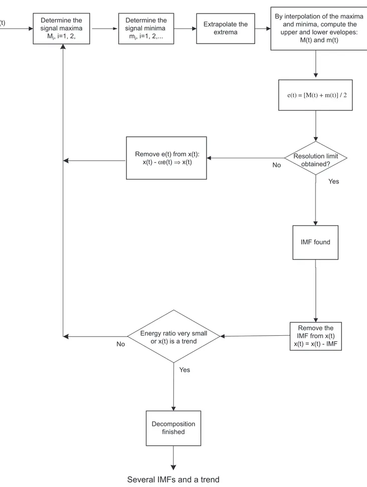
3.2.5. Flowchart of the algorithm
The EMD algorithm proposed here is summarized in the flowchart shown inFig. 2.
0 500 1000 1500 2000 2500 3000 3500 4000 4500
-10 0 10
0 500 1000 1500 2000 2500 3000 3500 4000 4500
-2 0 2
0 500 1000 1500 2000 2500 3000 3500 4000 4500
-2 0 2
0 500 1000 1500 2000 2500 3000 3500 4000 4500
-10 0 10
0 500 1000 1500 2000 2500 3000 3500 4000 4500
-10 0 10
0 500 1000 1500 2000 2500 3000 3500 4000 4500
-5 0 5
0 500 1000 1500 2000 2500 3000 3500 4000 4500
-10 0 10
x(t) Determine the signal maxima Mi, i=1, 2,
Determine the signal minima
mi, i=1, 2,...
Extrapolate the extrema
By interpolation of the maxima and minima, compute the upper and lower evelopes:
M(t) and m(t)
e(t) = [M(t) + m(t)] / 2
Resolution limit obtained?
Yes No
Yes No
IMF found
Remove the IMF from x(t) x(t) = x(t) - IMF Energy ratio very small
or x(t) is a trend
Decomposition finished
4. On the Hilbert spectral analysis
Spectral estimation is the second step of the HHT. This consists in computing the instantaneous amplitude and frequency for each IMF by using the HT and the analytic signal concept. This is another drawback of the HHT, because the HT uses the whole signal (theoretically from1toþ1). As we have a finite segment of a signal, the window effect will distort its spectrum and as a consequence its HT. As we will show later, this can give poor frequency estimation. Besides, it is not easy to accept a global operator as base for a local estimation. On the other hand, we do not need to estimate an instantaneous amplitude, because we already have it, as we will see next.
4.1. Demodulating the IMF
Let jðtÞbe an IMF andyðtÞthe corresponding analytic signal. So,
jðtÞ ¼RefjyðtÞjejargðyðtÞÞg ¼ jyðtÞjcos½yðtÞ, (3) where yðtÞ ¼arg½yðtÞ. So, we obtained an the instantaneous amplitude and an oscillating function that is a constant AM/FM signal (not necessarily a sinusoid). If jyðtÞj is known, we can perform an amplitude demodulation and obtain
sðtÞ ¼cos½yðtÞ, (4)
such that
jsðtÞjp1. (5)
sðtÞcan be considered as an FM signal. Its demodulation leads us to the instantaneous frequency. This will be considered in the next section. Now we will consider the amplitude demodulation.
At the end of the sifting procedure leading to the referred IMF,jðtÞ, we also have its envelopes, MðtÞand
mðtÞ. If these were the ‘‘true’’ envelopes, they would be symmetric and its difference would be the estimate of the amplitude modulating signal
jðtÞ ¼AðtÞ sðtÞ (6)
and
AðtÞ ¼ jyðtÞj ¼MðtÞ mðtÞ. (7) As MðtÞ and mðtÞ are not truly symmetric, we must look for a more reliable estimate of AðtÞ. This can be achieved by the following procedure:
(a) Make gðtÞ ¼ jjðtÞj.
(b) Compute the maxima of gðtÞ and extrapolate them as described in Section 3.2.2. (c) Interpolate those maxima to obtain an estimate ofAðtÞ.
Now, it is enough to divide jðtÞ byAðtÞ to obtain an FM signal,sFMðtÞ.
4.2. On the instantaneous frequency
Assume that the instantaneous frequency ofsFMðtÞis a slowly time varying signal, so that we may consider it
to be constant over small time intervals. Moreover, sample it to obtain a discrete-time signal that we can express in the format
sFMðnÞ cos½2pfðn0Þ:n (8)
valid for n0Npnpn0þN. So, we assume that the frequency is constant in a window with length 2Nþ1,
obtained from
cos½2pfðn0Þ ¼ PL1
2 sFMðnÞ½sFMðn1Þ þsFMðnþ1Þ
2PL1 2 s2FMðnÞ
, (9)
whereLis the number of available samples. In the case of a pure sinusoid this formula gives the correct value, provided we have at least three samples. For an FM signal we substitute L¼2Nþ1, as referred above. It defines the window of validity of the approximations. The choice ofNdepends on the practical application. In the case of the chirp signal presented in Section 5.2.1, we usedN ¼10. We have used values from 20 to 40 in EEG applications.
5. Illustrating results
5.1. EMD
5.1.1. Adding two IMFs
To illustrate the behaviour of the proposed algorithm and compare it with the original, we computed the corresponding decompositions for a signal that is a sum of two IMFs:
1. x1ðnÞ ¼sinð2pf0nÞ,
2. x2ðnÞ ¼2jsinð2pf1nÞj 1
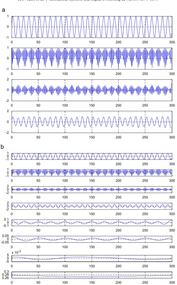
with n¼0;1;. . .;299, f1¼0:23 Hz. We made two trials withf0¼0:1 and 0.3 Hz. For comparison, we also
present the results obtained with Rilling’s routine [12]. In the following two figures, the signals in the upper two strips are the original signals. In Fig. 3, we present the results corresponding to the case of f0¼0:1 Hz. While our algorithm gives two IMFs, Rilling’s gives six.
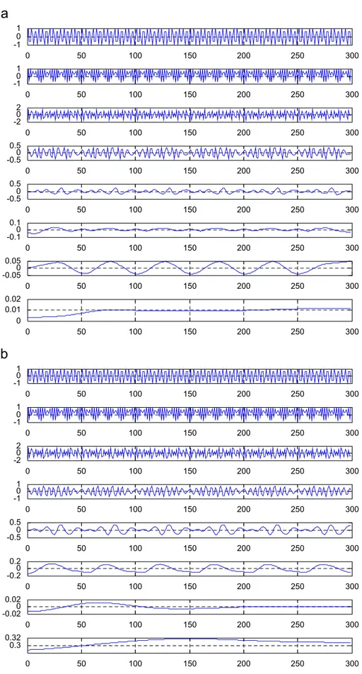
InFig. 4we show the results obtained with the same algorithms, but now with f0¼0:3 Hz. Now the results are similar: both decompose into six IMFs.
5.1.2. The chirp case
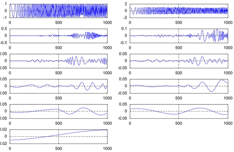
Another signal naturally fitting the IMF definition is the constant amplitude chirp signal. As the sampling period is fixed and the chirp frequency is time dependent, there is no way of obtaining a sequence with all the maxima with the same amplitude. We present the example of the chirp signal: cosð2pn2=4507þ2pn=213Þ, with
0pnp999. The chirp rests undecomposed under our modified EMD, but under Rilling’s EMD, a set of 10
IMFs is released as illustrated in Fig. 5. This is a non-desirable feature, because a signal already fitting the IMF definition should not be further decomposable.
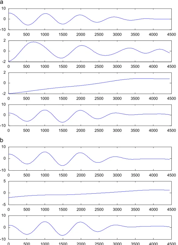
5.1.3. A robot movement signal
In the first strip of Fig. 6, we present the Y component of a horizontal movement of a robot and the corresponding EMD obtained with our and Rilling’s algorithms. Again, the results with our algorithm seem more plausible.
5.2. Frequency estimation
Each IMF appears as an AM/FM modulated signal. In Huang et al. papers [1,2] a Hilbert spectral estimation is used to estimate the instantaneous frequency. As said before, we suggest here the use of a local AR approximation to estimate the frequency through the first reflection coefficient.
5.2.1. Chirp signal
0 50 100 150 200 250 300 -1
0 1
0 50 100 150 200 250 300
-1 0 1
0 50 100 150 200 250 300
-2 0 2
0 50 100 150 200 250 300
-2 0 2
0 50 100 150 200 250
-1
300 0
1
0 50 100 150 200 250 300
-10 1
0 50 100 150 200 250 300
-20 2
0 50 100 150 200 250 300
-20 2
0 50 100 150 200 250 300
-0.10 0.1
0 50 100 150 200 250 300
-0.050 0.05
0 50 100 150 200 250 300
-50 5 x 10
-3
0 50 100 150 200 250 300
0.26 0.280.3
Fig. 3. Decomposition of the signal sinð2pf0nÞ þ2jsinð2pf1nÞj 1 using our and Rilling’s algorithms withf0¼0:1 Hz andf1¼0:23 Hz.
0 50 100 150 200 250 300 -10
1
0 50 100 150 200 250 300 -10
1
0 50 100 150 200 250 300 -20
2
0 50 100 150 200 250 300 -0.50
0.5
0 50 100 150 200 250 300 -0.50
0.5
0 50 100 150 200 250 300 -0.10
0.1
0 50 100 150 200 250 300 -0.050
0.05
0 50 100 150 200 250 300 0
0.01 0.02
0 50 100 150 200 250 300 -10
1
0 50 100 150 200 250 300 -10
1
0 50 100 150 200 250 300 -20
2
0 50 100 150 200 250 300 -10
1
0 50 100 150 200 250 300 -0.50
0.5
0 50 100 150 200 250 300 -0.20
0.2
0 50 100 150 200 250 300 -0.020
0.02
0 50 100 150 200 250 300 0.3
0.32
Fig. 4. Decomposition of the signal sinð2pf0nÞ þ2jsinð2pf1nÞj 1 using our and Rilling’s algorithms withf0¼0:3 Hz andf1¼0:23 Hz.
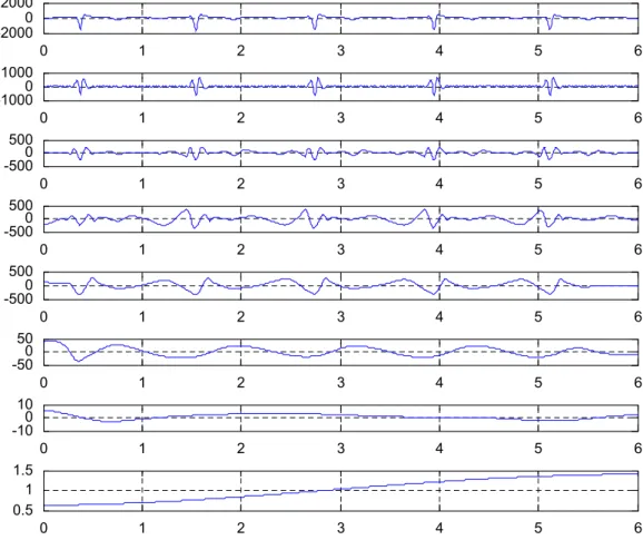
5.2.2. An ECG signal
In the following we will present the results concerning the analysis of a segment of an ECG signal with five beats. In Fig. 8 we present the original signal and the corresponding IMFs obtained with the algorithm we propose here.
For comparison we are going to present the results of the time–frequency analysis, using two algorithms:
Ours, that consists in the IMF amplitude demodulation followed by a frequency estimation using the AR modelling. Huang’s approach based on the HT.The energy operator demodulation proposed by Junsheng et al. [6] is not suitable to be used with short length signals since it cannot assure that the energy operator assumes only non-negative values.
As expected from our considerations in Section 4.1 the amplitudes are not very different (Fig.9). This does not happen with the frequency estimates. It is clear that our approach gives more realistic and convincing results, mainly in the frequency computation (Fig. 10).
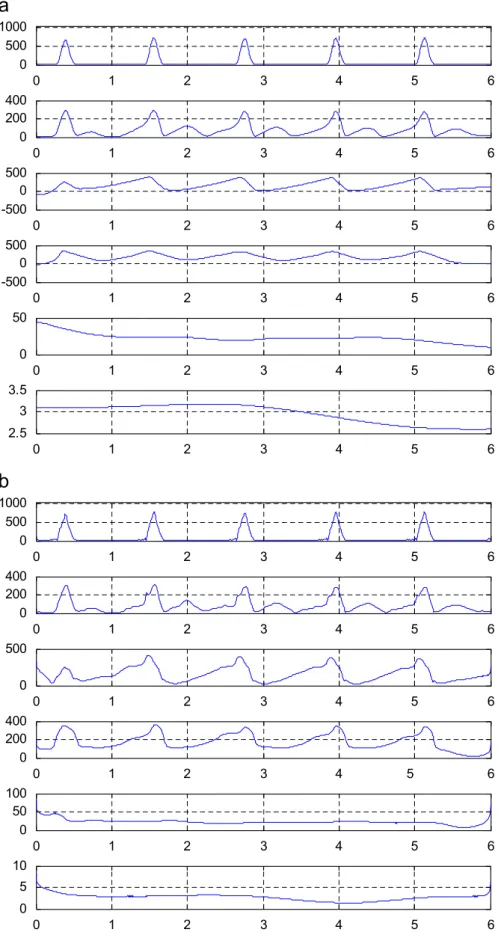
5.2.3. The temperature in a dryer
In Fig. 11 we present the time evolution of the temperature inside a dryer and its EMD using ours and Rilling’s algorithms.
Similar to the last example, we computed the amplitudes and frequencies for both the decompositions. In
Fig. 12 we present the results in a time–frequency plot. It seems clear that our algorithm seems to describe better the behaviour of the signal.
It is clear that the results stated inFig. 12a seem more plausible when we look at the signal we are studying.
0 500 1000
-1 0 1
0 500 1000
-2 0 2
0 500 1000
-0.5 0 0.5
0 500 1000
-0.1 0 0.1
0 500 1000
-0.05 0 0.05
0 500 1000
-0.05 0 0.05
0 500 1000
-0.05 0 0.05
0 500 1000
-0.05 0 0.05
0 500 1000
-0.05 0 0.05
0 500 1000
-0.05 0 0.05
0 500 1000
-0.02 0 0.02
Fig. 5. Original Rilling’s EMD of chirp signal cospn2=4507þ2pn=213, with 0pnp999. The interaction between the extrema locations
0 0.2 0.4 0.6 0.8 1 1.2 1.4 1.6 1.8 2 -0.1
0 0.1
0 0.2 0.4 0.6 0.8 1 1.2 1.4 1.6 1.8 2 -0.05
0 0.05
0 0.2 0.4 0.6 0.8 1 1.2 1.4 1.6 1.8 2 -0.02
0 0.02
0 0.2 0.4 0.6 0.8 1 1.2 1.4 1.6 1.8 2 -0.02
0 0.02
0 0.2 0.4 0.6 0.8 1 1.2 1.4 1.6 1.8 2 -0.05
0 0.05
0 0.2 0.4 0.6 0.8 1 1.2 1.4 1.6 1.8 2 -0.02
0 0.02
0 0.2 0.4 0.6 0.8 1 1.2 1.4 1.6 1.8 2 -0.1
0 0.1
0 0.2 0.4 0.6 0.8 1 1.2 1.4 1.6 1.8 2 -0.010
0.01
0 0.2 0.4 0.6 0.8 1 1.2 1.4 1.6 1.8 2 -0.050
0.05
0 0.2 0.4 0.6 0.8 1 1.2 1.4 1.6 1.8 2 -0.020
0.02
0 0.2 0.4 0.6 0.8 1 1.2 1.4 1.6 1.8 2 -0.050
0.05
0 0.2 0.4 0.6 0.8 1 1.2 1.4 1.6 1.8 2 -0.10
0.1
0 0.2 0.4 0.6 0.8 1 1.2 1.4 1.6 1.8 2 -0.020
0.02
0 0.2 0.4 0.6 0.8 1 1.2 1.4 1.6 1.8 2 -0.02
0 0.02
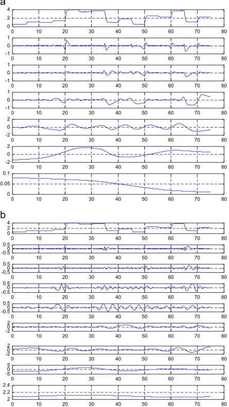
5.3. A brief comparison
The above results show that:
Our algorithm gives a small number of IMFs. Even at a glance, they seem to be more plausible as it is clear in the dryer case.0 100 200 300 400 500 600 700 800 900 1000 -4
-3 -2 -1 0 1 2 3 4
0 100 200 300 400 500 600 700 800 900 1000 0
0.05 0.1 0.15 0.2 0.25 0.3 0.35 0.4 0.45
Fig. 7. Estimation of the instantaneous frequency with Hilbert transform (a) and AR methods (b).
0 1 2 3 4 5 6
-2000 0 2000
0 1 2 3 4 5 6
-1000 0 1000
0 1 2 3 4 5 6
-5000 500
0 1 2 3 4 5 6
-5000 500
0 1 2 3 4 5 6
-500 0 500
0 1 2 3 4 5 6
-50 0 50
0 1 2 3 4 5 6
-100 10
0 1 2 3 4 5 6
0.5 1 1.5
0 1 2 3 4 5 6 0
500 1000
0 1 2 3 4 5 6
0 200 400
0 1 2 3 4 5 6
0 500
0 1 2 3 4 5 6
0 200 400
0 1 2 3 4 5 6
0 50 100
0 1 2 3 4 5 6
0 5 10
0 1 2 3 4 5 6
0 500 1000
0 1 2 3 4 5 6
0 200 400
0 1 2 3 4 5 6
-500 0 500
0 1 2 3 4 5 6
-500 0 500
0 1 2 3 4 5 6
0 50
0 1 2 3 4 5 6
2.5 3 3.5
0 1 2 3 4 5 6 -100
0 100
0 1 2 3 4 5 6
-100 0 100
0 1 2 3 4 5 6
-20 0 20
0 1 2 3 4 5 6
-10 0 10
0 1 2 3 4 5 6
-10 0 10
0 1 2 3 4 5 6
-10 0 10
0 1 2 3 4 5 6
0 20 40
0 1 2 3 4 5 6
0 10 20
0 1 2 3 4 5 6
0 20 40
0 1 2 3 4 5 6
0 50
0 1 2 3 4 5 6
0 2 4
0 1 2 3 4 5 6
0 1 2
6. Conclusions
The empirical mode decomposition as a data driven alternative approach to the analysis of non-stationary signals was described. We studied it and revealed its features and some drawbacks. Here we proposed
0 10 20 30 40 50 60 70 80
0 2 4
0 10 20 30 40 50 60 70 80
-0.50 0.5
0 10 20 30 40 50 60 70 80
-0.50 0.5
0 10 20 30 40 50 60 70 80
-0.50 0.5
0 10 20 30 40 50 60 70 80
-0.50 0.5
0 10 20 30 40 50 60 70 80
-20 2
0 10 20 30 40 50 60 70 80
-20 2
0 10 20 30 40 50 60 70 80
-50 5
0 10 20 30 40 50 60 70 80
2 2.2 2.4
0 10 20 30 40 50 60 70 80
0 2 4
0 10 20 30 40 50 60 70 80
-1 0 1
0 10 20 30 40 50 60 70 80
-1 0 1
0 10 20 30 40 50 60 70 80
-1 0 1
0 10 20 30 40 50 60 70 80
-2 0 2
0 10 20 30 40 50 60 70 80
-2 0 2
0 10 20 30 40 50 60 70 80
0 0.05 0.1
solutions for such difficulties in order to obtain an algorithm with better performances. We also criticized the use of the Hilbert transform for spectral estimation, presenting an alternative based on an AR local approximation. We also presented some simulation results.
Appendix A
Consider the signalsFMðtÞintroduced in Section 4.1. Assume that its instantaneous frequencyfðtÞis a slowly
time varying signal, so that we may consider it to be constant in small intervals. We can write
sFMðtÞ cos½2pfðt0Þ t (A.1)
for tin a small interval around t0. Sampling this signal we can express it in the format
sFMðnÞ cos½2pfðn0Þ:n (A.2)
valid forn0Npn0pn0þN. So, we assume that the frequency is constant in a window with length 2Nþ1.
In practice, we used N¼15. Here, we propose an instantaneous frequency estimator based on a local AR approximation. It is known that, if xn¼cosð2pfnþjÞ, with f 2 ð0;1=2 and j2(-p,p], it verifies an AR equation. In fact, we have
cos½2pfnþj ¼cos½2pfðn1Þ þjcosð2pfÞ sin½2pfðn1Þ þjsinð2pfÞ
and
cos½2pfðn2Þ þj ¼cos½2pfðn1Þ þjcosð2pfÞ þsin½2pfðn1Þ þjsinð2pfÞ. Adding both equations, we obtain
cos½2pfnþj þcos½2pfðn2Þ þj ¼2 cos½2pfðn1Þ þjcosð2pfÞ
and
cos½2pfnþj 2 cos½2pfðn1Þ þjcosð2pfÞ þcos½2pfðn2Þ þj ¼0 giving
xðnÞ 2 cosð2pfÞxðn1Þ þxðn2Þ ¼0 (A.3)
time (ms)
frequency (Hz)
0 10 20 30 40 50 60 70
0 0.005 0.01 0.015 0.02 0.025
time (ms)
frequency (Hz)
0 10 20 30 40 50 60 70
0 0.005 0.01 0.015 0.02 0.025 0.03
that leads to an AR model with polynomial
12 cosð2pfÞz1þz2. (A.4)
This polynomial is obtained using the Levinson recursion (see below) with the reflection coefficients:
C1 ¼ cosð2pfÞ (A.5)
and
C2¼1.
So, computing the first reflection coefficient in a window centred in the reference sample, we can obtain an estimate of the frequency.
Eq. (A.3) is a special case of the AR model
XN0
i¼0
aixðniÞ ¼vðnÞ, (A.6)
where vðnÞ is white noise andai,i¼0;1;. . .;N0, witha0 ¼1 are the AR parameters. These can be computed
from a set of reflection coefficients by means of the Levinson recursion (see below).
To compute the reflection coefficient estimates, we use a modified Burg method [10]. We are going to introduce it in the following steps. LetxðnÞ be a discrete time signal. ForN¼1;. . .;N0.
1. Define the forward and backward prediction errors by
fNn ¼X
N
i¼0
aNi xðniÞ (A.7)
and
bNn ¼X
N
i¼0
aNi xðnN1þiÞ (A.8)
and the error prediction power by
PN ¼ 1 2ðLNÞ
XL
Nþ1
½ðfNnÞ2þ ðbNnÞ2. (A.9)
2. Use the Levinson recursion[10]
aiN ¼aNi 1þCNaNN1i; i¼0;. . .;N (A.10) to obtain
fNn ¼fNn1þCNbNn1 (A.11)
and
bNn ¼bNn11þCNfNn11 (A.12)
withf0n¼xðnÞand b0n¼xðn1Þ.
3. With the above recursions, transformPNinto a function of a unique variable—the reflection coefficientCN:
PN ¼ 1 2ðLNÞ
XL
Nþ1
½ðfNn1þCN bNn11Þ
2þ ðbN1
n1 þCNfNn1Þ
2. (A.13)
4. DerivePN relative to CN and equate to zero to obtain
CN ¼
PL
Nþ2½f
N1
n b N1
n þf N1
n1b
N1
n1
PL
Nþ2½ðf
N1
n1Þ
2þ ðbN1
n Þ
2 . (A.14)
References
[1] N.E. Huang, Z. Shen, S.R. Long, M.L. Wu, H.H. Shih, Q. Zheng, N.C. Yen, C.C. Tung, H.H. Liu, The empirical mode decomposition and Hilbert spectrum for nonlinear and non-stationary time series analysis, Proceedings of the Royal Society of London A 454 (1998) 903–995.
[2] G. Rilling, P. Flandrin, P. Gonc-alves, On empirical mode decomposition and its algorithms, in: IEEE-EURASIP Workshop on
Nonlinear Signal and Image Processing NSIP-03, Grado (I), 2003.
[3] P. Flandrin, G. Rilling, P. Gonc-alves, On empirical mode decomposition as a filter bank, IEEE Signal Processing Letters 11 (2)
(2004).
[4] G. Rilling, P. Flandrin, On the influence of sampling on the empirical mode decomposition, in: Proceedings of the International Conference on Acoustics, Speech and Signal Processing, ICASSP 2006, pp. III-444–III-447.
[5] C. Junsheng, Y. Dejie, Y. Yu, Research on intrinsic mode function (IMF) criterion in EMD method, Mechanical Systems and Signal Processing 20 (2006) 817–824.
[6] C. Junsheng, Y. Dejie, Y. Yu, The application of the energy operator demodulation approach based on EMD in machinery fault diagnosis, Mechanical Systems and Signal Processing 21 (2007) 668–677.
[7] P. Maragos, J.F. Kaiser, T.F. Quatieri, On amplitude and frequency demodulation using energy operators, IEEE Transactions on Signal Processing 41 (4) (1993).
[8] S.R. Qin, Y.M. Zhong, A new envelope algorithm of Hilbert–Huang transform, Mechanical Systems and Signal Processing 20 (2006) 1941–1952.
[9] R.T. Rato, M.D. Ortigueira, A modified EMD algorithm for application in biomedical signal processing, in: Proceedings of the International Conference on Computational Intelligence in Medicine and Healthcare, CIMED 2005, Costa da Caparica, June 29–July 1, 2005 (CD edition).
[10] M.D. Ortigueira, J.M. Tribolet, Global versus local minimization in least-squares AR spectral estimation, Signal Processing 7 (3) (1984) 267–281.