A Work Project, presented as part of the requirements for the Award of a Master Degree in Economics from the NOVA School of Business and Economics
Euro Area Monetary Policy and Financial Stress Regimes:
A Threshold VAR Approach
Daniela Soares Martins
33081
A Project carried out on the Master in Economics Program under the supervision of Professor Luís Catela Nunes
1
Euro Area Monetary Policy and Financial Stress Regimes: A Threshold VAR Approacha
Abstract
We investigate how the state of financial conditions affects the transmission of monetary policy to the euro area macroeconomy. Our main goal is to analyze the responses of output growth and inflation to monetary policy shocks during periods of low and high financial stress. Results from a Threshold Vector Autoregression model show that monetary policy is of negligible importance to the real economy during normal times. However, an effective tool to ease the state of financial conditions when the economy is already facing strains. Empirical evidence also suggests that in the short-run monetary policy cannot significantly influence the inflation rate.
Keywords: Eurozone; Financial Stress Regimes; Monetary Policy Shocks; Threshold Vector Autoregression.
This work used infrastructure and resources funded by Fundação para a Ciência e a Tecnologia (UID/ECO/00124/2013, UID/ECO/00124/2019 and Social Sciences DataLab, Project 22209), POR Lisboa (LISBOA-01-0145-FEDER-007722 and Social Sciences DataLab, Project 22209) and POR Norte (Social Sciences DataLab, Project 22209).
a While assuming full responsibility for any error or omission, the author thanks Cynthia Wu for sharing their estimations for the ECB’s shadow rate, and Martín Saldías for suggesting the Krippner’s shadow short rate to the euro area along with the CISS as threshold variable. We are also grateful for Jasmine Zheng’s attention regarding the nonlinear estimation, and for the add-in from EViews’ community able to generate a Threshold VAR, following the seminal work of Balke (2000).
2
I. Introduction
Two well-known events of systemic stress in financial markets, the global financial crisis of 2007 and the sovereign debt crisis of 2010, have marked the brief history of the European Monetary Union. Both episodes helped to reverse a decade of steady economic growth and prompted deflationary pressures, threatening the ECB’s mandate for price stability. Worldwide, in the aftermath of the crises, macroeconomists turned their attention to the spillover effects of financial stress on the real economy as well as to what extent it can affect the transmission mechanism of monetary policy and, consequently, its effectiveness. Within this context, authors have been studying the effects on the transmission channels through which monetary policy acts (Dahlhaus, 2017), and how monetary policy was effective in “getting in the cracks”, albeit through nonstandard measures (Wu and Xia, 2016, and Inoue and Rossi, 2018).
In a theoretical framework, central banks follow monetary policy decisions, which in turn affect a wide range of financial variables that, afterward, act to transmit the policy changes to the real economy. It is pertinent to quote Bernanke (2007), “Monetary policy works in the first instance by affecting financial conditions, including the levels of interest rates and asset prices. Changes in financial conditions, in turn, influence a variety of decisions by households and firms, including choices about how much to consume, to produce, and to invest.”, which briefly summarizes the macro-financial linkages explored in this study.
The present study aims to extend current knowledge of potential nonlinear effects between monetary policy and financial stress to the euro area economy. Given this setting, we propose a nonlinear approach to capture how the state of financial conditions affects the transmission of monetary policy shocks to macroeconomic variables, namely output growth and inflation rates. Regarding the econometric methodology, a Threshold Vector Autoregression is estimated to model financial frictions and address three main questions:
3
2. How does the state of financial conditions react to unexpected changes in the monetary policy stance?
3. Is the price stability target for the inflation rate of below, but close to, 2 percentage points successfully attained through monetary policy shocks in the short-medium run?
Complementing the lively debate about the identification of monetary policy shocks in the aftermath of the zero nominal lower bound period and conduct of unconventional measures, we chose a shadow short rate as the monetary variable instead of a policy rate, monetary aggregates or, as more recently in the literature, the size of ECB’s balance sheet.
In this study, the threshold variable is included in the model and its critical value is estimated endogenously. Therefore, a shock to the financial conditions index, as well as to any of the other variables, can induce a switch in the regime. For the baseline model, we turn to a broad measure of financial stress, the ECB’s Composite Indicator of Systemic Stress (CISS), which places more importance in periods with stress prevailing in several market segments at the same time. Following this reasoning, an increase in the index corresponds to a deterioration in overall financial conditions, whereas a decrease reflects an improvement.
Our first set of results is obtained from a linear benchmark VAR model. Here we have an initial insight into the effectiveness of monetary policy to affect the state of financial conditions, with both variables, the shadow rate and the financial stress index, displaying a positive relationship in the medium-run. In addition, the qualitative response of inflation rate to monetary policy shocks introduces the concept of a cost channel effect of monetary policy, where a decrease in the external cost of funding (reflecting an easing of monetary conditions) passes through production, with output prices expected to decrease in return. Moreover, without even considering the role of financial frictions as a source of nonlinearities, output growth follows a delayed conventional response to monetary policy shocks.
Since all nonlinearity tests rejected the null hypothesis of linearity, there are reasons to believe that the data may present, in fact, nonlinear dynamics. The regime-dependent impulse response
4
functions derived from a Threshold-VAR model provide the second set of results. Here, the response of monetary policy to its own shock is amplified during stress periods than in normal times, supporting the estimation of nonlinear impulse response functions. We also find evidence that output growth responds in a greater extent to monetary policy shocks in the presence of financial strains. Once again, the results show an important role of monetary policy in easing financial stress when the economy is already in a state of deteriorating conditions.
The nonlinear impulse responses provide the last set of results, reflecting a mixed view from the previous two specifications. In line with empirical literature, there is evidence that output growth is more responsive to monetary policy shocks when the economy is initially in the high-stress regime. To that end, an intensification of the financial accelerator mechanism may be in place during stress periods, through the inverse relationship between a borrower’s creditworthiness and the “external finance premium”. This macro-financial linkage is also relevant to explain why monetary decisions are more powerful in affecting financial conditions when the economy is initially in a stress state. Once more, the response of inflation to a monetary shock is found to be quantitatively negligible. Empirical evidence suggests then a sluggishness of the prices in the euro area and an incapacity of monetary policy to affect the inflation rate in the short-medium run.
The remainder of this work is organized as follows. In section II we review literature on the linkages between financial frictions, monetary policy, and macroeconomy, along with a summary of recent research contemplating different measures for the monetary policy stance. Section III describes the followed empirical strategy, which includes a linear benchmark VAR model, and the model of interest, the Threshold-VAR. In section IV we define the dataset used and specification issues. Section V presents the estimated threshold value and the results from three specifications of impulse response functions on the relationship between monetary policy shocks and the state of financial conditions, along with a set of robustness checks. Section VI concludes with some policy implications from our empirical findings and some limitations of the pursued econometric
5
methodology. The method for computing the nonlinear impulse response functions is presented in Appendix A.
II. Revision of the literature
As remarked in Dahlhaus (2017), even though macroeconomists have not yet reached a consensus on the effects of financial stress, the last two crises for sure rekindled the motivation to analyze how a deteriorating state of financial conditions can impair a normal transmission of monetary policy to the real economy. Nonetheless, regarding macro-financial linkages exists a more consolidated literature to look upon.
Silvestri and Zaghini (2015) review some influential studies on the relationships between financial markets, and the rest of the economy. To that end, the authors highlight linkages, of which any appears to be present in the economic and financial history of the Eurozone and to be a plausible mechanism for our findings. One linkage refers to the inverse relationship between the (countercyclical) “external finance premium” and the (procyclical) net worth of borrowers, introducing the concept of the “financial accelerator” mechanism. As stated in Morley (2016), this mechanism supports the hypothesis that monetary policy can be an effective tool to offset financial or economic shocks.
The other linkage expands the previous mechanism to the financial intermediation channel, introducing agency problems into the model. The authors find empirical evidence that financial intermediaries act as important propagators of financial frictions. In this framework, Hartmann et al. (2015) critically appraise the CISS series’ construction since it includes a measure of instability in a market-segment of financial intermediation especially relevant in the euro area, retail banking. In an economy with an essentially bank-centered financial system, retail banks play a key role de facto in the transmission process of monetary policy, with the potential to enhance financial turmoil. After the recent financial crisis hit the Eurozone, one could observe a momentary blocking of ECB’s responses to alleviate stress and defend the Euro. At an early stage, the interest rate pass-through channel was being narrowed as policy changes were not being transmitted to the real
6
economy, leading to an unstable deviation in the retail rates from the policy ones (Holton and d’Acri, 2018).
There is a vast amount of literature on nonlinearities in the relationship between financial stress and monetary policy applied to the U.S. economy (Fry-McKibbin and Zheng, 2016, and Dahlhaus, 2017) and other economies with earlier established currencies (Li and St-Amant, 2010, and Saldías, 2017). Yet, previous work with nonlinear models applied to the euro area has focused on credit (Calza and Sousa, 2006) or financial conditions shocks (Hartmann et al., 2015; Silvestrini and Zaghini, 2015; and Tsagkanos, 2018).
When modeling nonlinear dynamics in monetary models, there exist several options for a switching variable, from the state of economic activity (Peersman and Smets, 2001, and Avdjiev and Zeng, 2014) to credit conditions (Balke, 2000, and Atanasova, 2003). However, the present study extends the works of Li and St-Amant (2010), Fry-McKibbin and Zheng (2016), and Saldías (2017) to the euro area, using a financial conditions index as the threshold variable. These studies found empirical evidence of threshold effects yet reached some conflicting conclusions.
For the U.S. economy, Fry-McKibbin and Zheng (2016) conclude a greater response from output to monetary policy shocks in the presence of financial strains. However, Saldías (2017) shows an opposite response, with the effect on output growth being stronger during normal times when the transmission mechanism of monetary policy is not impaired. In Canada, Li and St-Amant (2010) confirm the latter response only for contractionary monetary policy shocks. For expansionary monetary policy shocks, Fry-McKibbin and Zheng (2016) highlight the intensification of the cost channel effect in the short-run during periods of high financial stress, which results in a price puzzle with a decline of the inflation rate.
Regarding the response of financial conditions to monetary policy shocks, Saldías (2017) concludes that the effect is stronger in the stress regime. However, Li and St-Amant (2010), and Fry-McKibbin and Zheng (2016) converge on the same result: monetary policy displays a larger impact on the state of financial conditions when the economy is financially sound. Nonetheless,
7
Fry-McKibbin and Zheng (2016), and Saldías (2017) remark the effectiveness of expansionary monetary policies in easing financial conditions when the economy is in the high-stress state.
Concerning the choice of the baseline threshold variable, a considerable range of macro-financial literature uses the ECB’s Composite Indicator of Systemic Stress (CISS) as a measure of the state of financial conditions (Mittnik and Semmler, 2013; Hartmann et al., 2015; Tsagkanos et al., 2018; among others). In the present study, similar to Hubrich and Tetlow (2015), although a threshold value for the financial conditions index is estimated to distinguish periods of low- and high-stress, the interest does not lie in the level of the variable but on its interaction with the proposed macro and monetary variables.
In line with recent research, we stand out from the traditional identification of monetary policy shocks, turning to a well-known shadow rate (Wu and Xia, 2019). As key policy rates approached zero and unconventional monetary measures were implemented, an array of alternative measures has emerged to better capture the overall changes in the monetary policy stance.
For instance, Wu and Xia (2016) propose a shadow rate for the U.S. economy in order to overcome the inertia of the federal funds rate at the zero lower bound (ZLB).b The authors
concluded that their artificial interest rate displays dynamic correlations with macroeconomic variables after the Great Recession similar to the ones from before with the policy rate. This result is particularly useful nowadays since it enables the update of previous empirical models that relied on short-term interest rates to identify monetary policy shocks. Following the same research question, Damjanović and Masten (2016) focus on the euro area, specifying a VAR model with the shadow short-term interest rate of Krippner (2015) as the measure for policy stance.
Francis et al. (2019) compare different alternatives for the identification of monetary policy shocks from the short-term rate to the Fed’s balance sheet size and shadow rates, testing for both
8
Wu-Xia and Krippner.c Their results conclude no relevant differences between the two artificial
rates, but either one performed better than the policy rate when considering the ZLB period. Considering other works in the literature, Saldías (2017) resorts to the yield curve slope, whereas Inoue and Rossi (2018) identify monetary policy shocks as shifts in the whole term structure of government bond yields, focusing on more two factors: the level and the curvature.
III. Methodology
In this section, we describe our econometric methodology, which is divided into two subsections: the estimation of a benchmark VAR and the model of interest, the Threshold-VAR. Here, the standard VAR is a system of four regressions estimated by OLS with each set of variables regressed on its lagged values and the ones from the other three variables.
A. Benchmark VAR
Following Atanasova (2003), before nonlinear modeling, we estimate a Linear Vector Autoregression model as a starting point to analyze the relationships between the proposed variables, specified as:
𝑌 = 𝑐 + 𝐴𝑌 + 𝐵(𝐿)𝑌 + 𝑢 (1)
where 𝑌 is the vector of endogenous variables, 𝑐 the vector of intercepts, 𝐴 the matrix of structural contemporaneous relationships, 𝐵 the matrix of lagged coefficients and 𝑢 the vector of structural shocks.d Accounting for potential structural breaks, several specifications of the VAR model are
estimated for robustness purposes. First, we estimate the model solely with three variables (output growth, inflation, and the shadow rate) excluding the market stress. The estimation is done for the whole sample and for the periods preceding and succeeding the hit of the global financial crisis, not capturing yet nonstandard monetary policies. Second, the stress variable is introduced in the model, and the previous estimation procedure is followed again.
c As a robustness check, the same procedure was pursued in the present study. The results did not significantly differ between the two specifications.
9
i. Linear impulse response functions
In order to analyze how shocks to monetary policy affect the economy in the short-medium run, we calculate the impulse response functions. One describes the response of a variable 𝑦 throughout the horizon of response to a one-time impulse at time t in our structural shock with all the other variables held constant. The computation of the linear impulse response functions is of less complexity than nonlinear and can be defined as the change in the conditional expectation of y as a result of a shock 𝑢 :
𝐼𝑅𝐹 (𝑛, 𝑢 ) = 𝐸[y |𝑢 ] − 𝐸[y ] (2)
Assuming a recursive (Cholesky) ordering for the identification scheme as real output growth (it), inflation rate (ht), Wu-Xia shadow rate (rt), and the financial stress index (st), we identify the
structural disturbances by shocks to the shadow rate equation in the VAR system, corresponding to the unexpected changes in the stance of monetary policy.
it → ht → rt → st (3)
A similar causal ordering to (3) is applied in Fry-McKibbin and Zheng (2016), Silvestrini and Zaghini (2015), and Mallick and Sousa (2013) who also include a measure of financial market stress in their models. Hence, the present study remains faithful to conventional shock identification with the form: output, prices, monetary policy, and financial market variables. Under this ordering, a monetary policy shock has an instantaneous impact on the financial stress index, however, output growth and inflation react with a lag. It is worthwhile noting that ordering the stress indicator last corroborates the idea that the ECB’s mandate does not impose an instantaneous response to shocks in the financial market stress.e
B. Threshold VAR
In order to study how the state of financial conditions affects the transmission of monetary policy shocks to macroeconomic activity, a multivariate Threshold Vector Autoregression (TVAR)
e Following Kremer (2016), we tested the model with an alternative structural ordering, where the shadow rate is ordered last. The results remained consistent. Nevertheless, it should be noted that the construction of the FCI incorporates individual indicators likely related to unexpected changes in monetary policy, which corroborates ordering it after the monetary variable.
10
model is estimated, which allows for regime-dependent and asymmetric responses to the shocks. Given the limited amount of usable observations, only two regimes associated with changes in the financial conditions index are assumed, “low-stress” and “high-stress”.f
Following the notation of Balke (2000), the “structural” Threshold VAR model can be specified as:g
𝑌 = 𝑐 + 𝐴 𝑌 + 𝐵 (𝐿)𝑌 + (𝑐 + 𝐴 𝑌 + 𝐵 (𝐿)𝑌 )𝛪(𝑠 > 𝜏) + 𝑢 (4)
where 𝑌 is the vector of endogenous variables, 𝐵 (𝐿) and 𝐵 (𝐿) the lag polynomial matrices representing the dynamics of the Threshold-VAR system, 𝑐 and 𝑐 the vectors of intercepts and 𝑢 structural errors. The threshold variable (𝑠 ) is a financial conditions index, reflecting the two states of financial stress. 𝛪(𝑠 > 𝜏) is an indicator function that equals 1 if 𝑠 is greater than a threshold value 𝜏 (high-stress regime), and 0 otherwise (low-stress regime). As proposed in Holló et al. (2012), the maximum threshold lag d can be of two months.h Besides allowing lag
polynomials to change across regimes, the “structural” contemporaneous relationships 𝐴 and 𝐴 can vary as well. To identify the structural Threshold-VAR model, we assume the same recursive structure as mentioned before in (3).
The model is estimated by ordinary least squares for each equation of the VAR and the chosen lag length is four, determined by minimizing the Akaike Information Criterion (AIC). The threshold value τ is not known beforehand and is estimated as the one that maximizes the log determinant of the “structural” residuals. For this purpose, the grid search over the possible values of τ is restricted to ensure that each regime contains at least 15% of total observations.
f See Avdjiev and Zeng (2014) for a three-regime Threshold-VAR describing the interactions between credit market, monetary policy, and macroeconomic activity over the business cycle.
g Balke (2000) defines the model as “structural” because it imposes a block-recursive structure based on a standard Cholesky decomposition.
h The model was tested for both specifications, however the differences between the two were irrelevant. Thus, in order to be more parsimonious, we stuck with the default value of 1 for the delay lag. Also note, since the CISS series is not too erratic, only a moving average of order 1 is considered. We found that it properly distinguishes “stress events” from “normal times”.
11
i. Nonlinear impulse response functions
Once the TVAR model is estimated, we derive the nonlinear impulse response functions, which allow for regime-switching throughout the horizon of response to the shock. Therefore, these differ from the linear ones since the responses are not bound to symmetry and are dependent on the history of shocks as well as on the sign and size of the shock.
Following Balke (2000), the generalized impulse response functions (GIRF) are computed through bootstrap simulations.i These may be defined as the difference between the forecasted
path at horizon n of the variable in the presence and in the absence of a shock to the variable of interest, dependent on the initial conditions at the time of the shock falling under one of the two regimes (Tsagkanos, 2018). The nonlinear impulse responses can be specified as:
𝐺𝐼𝑅𝐹 (𝑛, 𝑢 , Ω ) = 𝐸[y |𝑢 , Ω ] − 𝐸[y |Ω ] (5)
where 𝑛 is the forecasting horizon, Ω is a particular history at time 𝑡 − 1 and 𝑢 an unexpected one-time shock at time 𝑡 to the endogenous variable of interest.
In the results section, we present the GIRFs for shocks to the shadow rate of different sign and magnitude, namely of ±1 standard deviation and ±2 standard deviation, and conditional on the two possible initial regimes of low and high financial stress.
IV. Data and specification issues
Our assessment focus on the euro area with a fixed country composition (EA-12) – the 11 original countries plus Greece. The subsequent enlargement countries were excluded from the analysis given their late entry in the euro area and relatively small GDP-weight in the EA-19. Thus, the aggregate data is computed as GDP-weighted averages of individual statistics.
The baseline model is estimated using monthly series of real output growth, inflation rate, the Wu-Xia shadow rate, and the preferential stress variable, the Composite Indicator of Systemic Stress (CISS). The sample starts in 1999M01 since the CISS series is not available before the official launch of the euro. For the output growth, we use the index of industrial production
12
collected from OECD.Stat. For inflation, we use the annual growth rate of the Harmonized Index of Consumer Prices (HICP) excluding energy prices from the ECB’s Statistical Data Warehouse.j
Both series are seasonally adjusted and transformed by taking annual natural logarithmic differences, as in Kremer (2016).
Even though the inflation and shadow rates series have a unit root, they were not transformed to attain stationarity.k To overcome the concern of possible spurious results, our approach was
based on Ashley and Verbrugge (2009). Through Monte Carlo simulations, the authors show that VAR models in levels, instead of differencing I(1) variables, perform adequately when retrieving the impulse response functions.l
A. Measuring the monetary policy stance
In the aftermath of the financial crisis of 2007, the ECB started to reduce policy interest rates, complementing with nonstandard monetary policy measures.m The subsequent sovereign debt
crisis of 2010 reinforced the easing of monetary conditions, providing further liquidity in order to reduce the strains in financial markets. Thus, in the past decade, the short-term policy rate has become insufficient to capture the major changes in the stance of monetary policy. Using it as a solo instrument would risk undervaluing the ECB’s actions, which aimed to contain market frictions and, consequently, revert an economic slowdown that was threatening the price stability mandate through deflationary pressures.
For the purpose of identifying the stance of monetary policy, Wu-Xia shadow rate for the euro area was used as a proxy, capturing not only the conventional instruments but also forward
j To this date, the range of seasonally adjusted HICP series is solely available for the euro area with changing composition. Therefore, in order to consider the weight of Greece before 2001M01, first we collect the HICP series from Eurostat, which is available for each country; second, we treat it through the X-12 ARIMA procedure to remove seasonality; and, finally, weighted-adjust the ECB’s overall statistic for the Greece’s now seasonally weighted-adjusted HICP series. The same procedure is followed with the purpose of extracting the weighted enlargement’s statistics after 2007M01.
k As a robustness check, the model is estimated with the I(1) variables transformed in first differences. These results can be found in Appendix C. Figure 5 and Figure 6.
l See also Toda and Yamamoto (1995), and the seminal contributions of Eric Sims (2011) for a validation of the use of VARs in levels if one wants to recover impulse responses. The VAR model (or the threshold alternative) should have at least two autoregressive lags in order to allow for standard tests and confidence intervals on the coefficients, which are later on an input to the estimation of the impulse response functions (Dolado and Lütkepohl, 1996).
13
guidance and large-scale asset purchase programs (APP).n Wu and Xia (2016) show, after the
Great Recession, a similar interaction of shocks to the shadow rate with the economy, as the policy rate exhibited before. This result is of extreme importance in the present study since it requires a series able to identify monetary policy shocks in a sample with a long period characterized by extremely low and inert policy rates, and packages of unconventional measures.
As a robustness check, our model was also estimated with the shadow short-term rate proposed in Krippner (2015).o Both shadow rates approximate the policy rate during normal times, having
the possibility however to turn negative in the presence of the zero nominal lower bound or unconventional measures.p Although the latter satisfies the stability condition in the proposed
linear VAR models (see Section III. A), we believe that the shadow rate by Wu and Xia (2019) represents more accurately the orientation and concrete decisions of ECB’s monetary policy, particularly in the past three years (see Appendix C. Figure 2). Notwithstanding, the results between the two specifications are not qualitatively different.q
B. Measuring financial stress
The baseline model uses ECB’s Composite Indicator of Systemic Stress (CISS) in the financial system as the threshold variable. As stated in Duprey et al. (2017), it represents the benchmark FCI for the Eurozone and aims to measure the financial instability in the main sources of funding in the euro economy. More specifically, the CISS explores the role of the banking sector, especially relevant in the euro area where it still plays a crucial role in economic activity.
Even though being a nonstationary series, the variable chosen as the threshold was not transformed. r Taking the first differences would result in a too erratic series, thus not appropriate
n To this date, the Wu-Xia SR is only available after 2004M09. However, prior to 2009, it is closely followed by the EONIA market rate (see Appendix C. Figure 2). Assuming that, before 2004M09, the ECB’s policy rate was transmitted to the overnight interbank rate without disturbances, the missing data is computed through interpolation. Also note that Wu and Xia (2016) rely on an overnight rate to construct the SR for the U.S., making it logical for the euro SR to follow the EONIA.
o The SSR developed by Krippner (2015)is publicly available on the Reserve Bank of New Zealand website.
p Even though in June 2004 an ECB’s key interest rate (MDF) entered negative territory, we gave preference to a shadow rate. The latter presents a behavior not so inert and enables us to capture the unconventional dimension of monetary policy.
q There is a minor difference in the high-stress regime: the response of stress to a shock on the Krippner rate only after ten months follows the one resulting from the baseline model.
14
to define accurately regime-switches. Moreover, as presented in the section of robustness analysis, the estimated model with I(1) variables in first differences, even considering a moving average of higher-order to smooth the fluctuations, still identified some high-stress events that from a historical perspective were not reasonable.
FIGURE 1. The Composite Indicator of Systemic Stress (CISS), its estimated threshold value (0.231634), and historical systemic stress events in the Eurozone.
Source: ECB’s Statistical Data Warehouse and authors’ calculations. From Figure 1, which plots the CISS raw series and its estimated threshold value, we conclude that the stress variable in levels is the most appropriate to incorporate in the baseline model, to test for threshold effects and to identify financial stress events. One can see that the vertical lines, which highlight historical systemic stress events in the Eurozone, coincide with the increases and peaks of the financial conditions index raw series. Yet, when using FCIs as indicators of financial stress, robustness checks with other indexes are recommended. Therefore, in the section of robustness analysis, we analyze the model with two other alternatives: the Bloomberg FCI for the euro area and the Country-Level Index of Financial Stress.s
V. Empirical results
Before proceeding to the analysis of the results, note that the variables in rates are displayed as number (for the first three variables, a response of 0.001 equals 0.1%), and the IRFs are displayed with a 68% confidence level which corresponds to one-standard error confidence bands. The latter procedure is not uncommon in VAR literature. The following results are divided into five
15
subsections: A) the estimated threshold value and the results of linearity tests; B) the impulse response functions from the benchmark VAR model; C) the regime-dependent impulse response functions derived from the baseline TVAR model; D) the generalized nonlinear impulse response functions for the TVAR; E) robustness analysis.
A) Estimating the threshold value and testing for nonlinearity
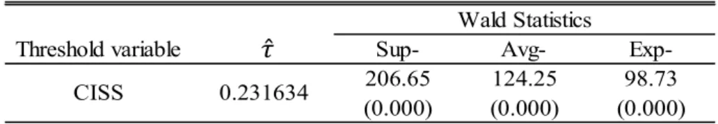
Table 1 reports the estimated threshold value for the CISS and the results of three nonlinearity tests. All tests reject the null hypothesis of linearity in the relationships between the times series. Since threshold effects appear to be present, a constant-parameter VAR reflecting a single-regime may not be the most adequate specification to describe the dynamics in financial stress, monetary policy, and economic activity.
TABLE 1. The estimated threshold level and Wald tests for nonlinearity.
NOTE: Ho: No difference between a linear VAR model and a threshold specification. The values in brackets are the asymptotic p-values computed when a parameter is not identified under the null hypothesis, through the simulation method of Hansen (1996).
When the level of the financial conditions index surpasses 0.231634, the euro area economy is in a regime of “high” financial stress; otherwise, it is in a regime of “low” financial stress (or “normal conditions”). From Figure 1 in the previous section, one can see that the estimated model is in the low-stress regime for most of the sample considered. From a long historical perspective, stress events are rather infrequent; therefore, this result does seem plausible. It can also be noted that the estimated threshold value accurately identifies the main systemic events in the history of the euro area, from the Subprime Mortgage Crisis in 2007, and subsequent fall of Lehman Brothers in 2008, to the Eurozone Debt Crisis in 2010.t
B) Linear impulse responses
Figure 2 shows the IRFs to a monetary policy shock for the benchmark specification, which admits no distinct states of the economy and no regime-switching. It considers a negative one standard
t Following the definition proposed in Holló et al. (2012), “systemic” stress reflects the materialization of the risk in which financial instability is not market-specific and becomes so widespread that impairs the “normal functioning” of financial markets. The distorted transmission channels from the financial system, consequently, affect the health of real economic activity, through the decisions of consumption and investment.
Threshold variable Sup- Avg- Exp-CISS 0.231634 206.65 (0.000) 124.25 (0.000) 98.73 (0.000) Wald Statistics 𝜏̂
16
deviation shock to the shadow rate (here, interpreted as an unanticipated easing of monetary policy) over a two and half years’ horizon of response. According to the first plot, the output growth follows a hump-shaded path, with the expected expansionary effect only occurring one year and three months after the shock.
The estimated response of the inflation rate seems “counterintuitive” as, after four months of the shock, the variable starts a declining path throughout the forecasted horizon, achieving a maximum break one and half years after the shock. The reason for the response of inflation to the monetary policy shock may lie on cost channel effects, which may be dominating the demand channel of monetary transmission.u The latter channel is the one that supports the conventional
response of prices to monetary policy, where an easing of monetary conditions induces an expansion of aggregate demand that afterward increases inflation. Nevertheless, note that the effects on the inflation rate are quantitatively negligible, with the maximum impact corresponding to an absolute difference of 0.04 percentage points relative to what would be expected in the absence of the shock.
From the last plot, one can see that monetary policy has relevant effects on financial conditions. The easing of monetary conditions leads to a decrease in financial stress, with the response turning significant after ten months. The benchmark VAR provides an insight that expansionary monetary policies appear to be an effective tool in containing financial stress. Our results reflect then a short-run positive relationship between the two variables. One should also note that the CISS series is a measure of systemic risk that has already materialized, and so it does not fully capture the build-up of potential financial vulnerabilities that may be allied with a monetary policy too much loose. This caveat explores a topic that goes beyond the scope of this study but is introduced on Saldías (2017). The author ponders if engaging in “lean against the wind” policies, as a means to contain the heating of the economy, is or not beneficial.
u Exists empirical literature which justifies the use of a commodity price index in order to overcome the “price puzzle” normally encountered between monetary shocks and prices. However, in the present study, we applied the order proposed in Mallick and Sousa (2013), with the ECB’s Commodity Price Index ordered after the inflation rate, and the results did not differ.
17
The IRFs remained robust with the different specifications for the linear VAR as proposed in Section III. A. However, when splitting the sample in the pre- and post-crisis periods, a slight difference was found in the response of output growth to monetary policy shocks.v For the
post-crisis model, the conventional response of output to monetary policy is more sluggish relative to the benchmark specification. Here, the expected response only happens in twenty months after the time of the shock instead of fifteen months as mentioned above.w One possible reason for this
difference could be an impairment of the transmission channel of monetary policy shocks to output growth, after the hit of the global financial crisis of 2007, through uncertainty or distrust issues from economic agents (Saldías, 2017).
FIGURE 2. Impulse response functions from a linear VAR(4): Impact of a one standard deviation negative shock to the shadow rate over 30 months.
NOTE: The model is estimated from 1999M01 to 2019M08. Dotted lines are the respective one-standard error confidence bands, corresponding to a 68% confidence level.
C) Regime-dependent impulse responses
As a second step, Figure 3 shows the estimated conditional linear impulse responses derived from the Threshold-VAR model for each financial stress state. These still do not allow for asymmetric responses or regime-switching, i.e., the economy is bound to stay in the same regime as it initially was at the time of the shock. Therefore, the shocks are history independent and the responses are linear inside each regime.
v The impulse response functions for the different specifications can be shared upon request.
wThe pre-crisis model retrieves faster the conventional response of output to monetary policy. With this model, only after six months of the time of the shock, the IRF of output growth to the shadow rate shock displays the expected response, instead of the longer period of fifteen months from the benchmark specification.
18
FIGURE 3. Regime-dependent impulse response functions derived from a TVAR(4): Impact of a one
standard deviation negative shock to the shadow rate conditional on a regime of low or high financial stress over 30 months, admitting no regime-switching and no asymmetric responses to an expansionary monetary policy shock.
NOTE: The low-stress regime shock was rescaled to equate the size of the shock in the high-stress regime. Black lines refer to the low-stress regime. Grey lines refer to the high-stress regime. Dotted lines are the respective one-standard error confidence bands.
In order to facilitate comparisons, the responses of the shadow rate to its own shocks were normalized across regimes by rescaling the size of the low-stress regime shock (0.23 p.p.) to that of the high-stress regime (0.34 p.p.). If the behavior of the system within each regime significantly differs from one another, the conditional linear impulse responses give a first impression into the usefulness of estimating the nonlinear functions. From the four plots, differences across regimes can be perceived. Even before normalization, the shadow rate is detected to be more sensitive in the high-stress regime than in the low one, reflecting a more active response of monetary policy when the economy is experiencing financial strains than in “normal times”.
Regarding output growth, the effects are negligible in the low financial stress regime. This result highlights a short-run monetary neutrality where, in the absence of high financial stress, monetary policy cannot influence the course of the real economy. However, when the economy is in a deteriorating state of financial conditions, output growth is predicted to follow a hump-shaded path, with the expected effect of a monetary policy expansion lagged in eight months. Thereafter, one and a half years past the time of the shock, output growth reaches a maximum difference of
19
0.63% as would be in the absence of the shock. Here, there is a first insight that output growth reacts in a greater extent to monetary policy shocks in periods of high financial stress.
Concerning the response of the inflation rate in the low-stress regime, inflation seems to follow the conventional response only until a year after the shock. Afterward, the response becomes minimal relative to the one from the high-stress regime. For the high-stress regime, it seems to follow with a lag of four months the response of economic activity to the shock. Therefore, in the presence of financial strains, the conventional response of prices to monetary policy happens only one year after the time of the shock. This last result reflects a lagged dominance effect of the monetary transmission demand channel over the cost channel (Fry-McKibbin and Zheng, 2016). Nevertheless, as mentioned in the previous subsection, the effects on inflation are again quantitatively negligible.
Once more, monetary policy proves to be a useful tool to contain financial stress when the economy is already in the high-stress regime. The declining response of financial stress to an expansionary monetary shock turns significant half a year past the time of the shock. With low-stress, one can notice a peak response on impact of financial stress to a loosening of monetary conditions. This result may reveal a build-up of financial vulnerabilities coming from a well-functioning economy allied to a much-eased monetary policy that is momentarily noticed by financial markets. Overall, the four variables are more responsive to monetary policy shocks in the high financial stress regime than in the low-stress regime, which gives us reasons to estimate the nonlinear impulse responses.
D) Nonlinear impulse responsesx
Admitting that a shock to monetary policy can induce a switch in the regime through its effects on the financial conditions variable, Figure 4 and Figure 5 plot the generalized impulse response functions, for different specifications of the direction and magnitude of the shock, conditional on an initial regime of low- or high-stress, respectively.
x Unfortunately, concerning the nonlinear impulse response functions, confidence bands cannot be displayed in this study for software’s unavailability. Therefore, only an analysis of the responses is followed, without referring to the results’ significance.
20
FIGURE 4.Generalized impulse response functions from a TVAR(4): Impact of a ±1 and ±2 standard
deviation shock to the shadow rate over 30 months conditional on an initial regime of low financial stress.
NOTE: Grey lines refer to expansionary monetary policy shocks (decline). Black lines refer to contractionary monetary policy shocks (increase). Dotted lines reflect a shock-width of ±1 standard deviation. Solid lines reflect a shock-width of ± 2 standard deviation.
FIGURE 5. Generalized impulse response functions from a TVAR(4): Impact of a ±1 and ±2 standard deviation shock to the shadow rate over 30 months conditional on an initial regime of high financial stress.
NOTE: Grey lines refer to expansionary monetary policy shocks (decline). Black lines refer to contractionary monetary policy shocks (increase). Dotted lines reflect a shock-width of ±1 standard deviation. Solid lines reflect a shock-width of ± 2 standard deviation.
21
Even though the responses are nearly symmetrical regarding the sign and size of the monetary policy shock, they differ for each initial state of the financial conditions index. The overall responses are more sensitive in the initial state of high-stress than in normal times, with financial strains empowering the shocks to monetary policy. For the initial regime of low-stress, the conventional response of the output growth to monetary policy only happens two years after the shock. Nevertheless, monetary policy seems unable to stimulate or deprive real economic activity in "normal times”, as the responses are quantitatively minimal. For the initial regime of high-stress, the expected effect of a contractionary monetary policy happens earlier, only eight months after the shock. Thereafter, output growth is expected to be less than it would be in the absence of the shock.
Qualitatively, in the high-stress regime, the cost channel effect of monetary policy dominates the demand channel throughout the forecasted horizon (Fry-McKibbin and Zheng, 2016). In the low-stress regime, the cost channel effect only takes over one year after the shock. Nonetheless, as remarked in Moccero et al. (2014), for the majority of the sample considered, prices in the euro area have been sluggish. In the present study, that remark is called for attention since the inflation responses to the shadow rate shocks are quantitatively negligible for both regimes. One can then induce that monetary policy shocks seem incapable to influence the inflation rate in the short-medium run.
Also with this specification, the empirical evidence suggests monetary policy as a determinant instrument to ease stressed financial conditions.y Similar to the conclusions in Dahlhaus (2017)
and Saldías (2017), our results show that the responses of the financial conditions index to monetary policy shocks are more reactive in the high-stress regime than in the low one. This result can be linked to the financial accelerator mechanism, which is strengthened in the presence of financial frictions and, consequently, empowers the decisions of monetary policy (Fry-McKibbin
22
and Zheng, 2016). When the economy is facing financial strains, consumption and investment are more constrained through a decline in cash flows, but also the option of leverage is more restricted. More specifically, the cost of external funding increases as the borrowers’ creditworthiness decreases and the risk perceived is normally higher than in “normal times” of credit. As the net worth of borrowers decreases, with the cash flows’ decline deteriorating the balance sheets and, consequently, the borrowers’ financial positions, the size of the “external finance premium” increases. Therefore, changes in the stance of monetary policy during stress events, through the provision of liquidity to money markets or cuts in the policy rates, reduce the liquidity risk and stimulate credit growth, directly translating into large changes in the cost of credit to households and firms. From a historical perspective, as mentioned in the literature section, retail banks and other financial intermediaries were initially reluctant to transmit directly the cuts in policy rates to loan rates; however, the implementation of unconventional measures of monetary policy helped to reduce the perception of risk and build more optimistic macroeconomic projections, therefore easing the stressed credit conditions. The actions of quantitative easing and forward guidance were also important in reducing the pressures from financial markets on the most distressed sovereigns in the Eurozone, avoiding then a bigger compromise of public budgets in order to repay debt or pay unsustainable debt services.
The estimated nonlinear impulse responses to shocks in monetary policy display symmetrical behavior within each regime, therefore the transition probability appears not relevant here, counterpointing similar studies where the sign (Li and St-Amant, 2010) or size of the monetary shocks (Fry-McKibbin and Zheng, 2016) revealed disproportional effects on output, inflation, and financial stress. Here, the responses to monetary policy shocks reveal no asymmetrical differences between expansionary or contractionary monetary policy shocks (Weise, 1999, and Atanasova, 2003), neither between small or large shocks (Li and St-Amant, 2010). Yet, the estimated model highlighted a variable whose shocks are more likely to induce a regime-transition, the stress variable. Relative to monetary shocks, the impulse response functions to shocks in the financial
23
conditions index are asymmetrical (Appendix C. Figure 3 and Figure 4). It appears that an unexpected change in the financial conditions index resembling an increase in financial stress is more likely to induce a switch in the low-stress regime to the high-stress than the other way around, suggesting an asymmetrical response to bad news over the state of financial conditions relative to good ones. To sum up, if one were to consider the financial conditions index as the variable of interest, the transition probability would be extremely valuable.
E) Robustness analysis
The model with the I(1) variables transformed in first differences also detected threshold effects, the nonlinearity tests for this specification can be found in Appendix B. Table 1. To compare the results with the baseline model, the cumulative response functions are calculated. Figure 5 and Figure 6 in Appendix C. plot the responses for the model with stationary variables conditional on each initial state. The main qualitative conclusions remain with this specification; however, slight differences appear before the responses cross the horizontal axis.
Regarding other threshold alternatives, Appendix C. Figure 1. (A) shows the estimated threshold level for the Bloomberg FCI, where the indicator function equals 1 if the threshold variable 𝑠 is less than the threshold 𝜏, and 0 otherwise. The results remain robust considering this specification for the threshold variable (Figure 7 and Figure 8 in Appendix C.); however, the responses’ asymmetry between regimes appears not as enhanced as with the CISS specification. Appendix C. Figure 1. (B) plots the threshold structure identified for the CLIFS specification and one can see that it does not spot well the marked historical stress events.z Consequently, we chose
not to display the estimated impulse response functions for this specification. VI. Concluding remarks
We parted from a standard linear VAR model, with the Threshold development afterward in order to cover nonlinearities that, according to economic theory, may be present in macroeconomic times
z Since the CLIFS is a measure of systemic stress only available for singular countries, the presented failure may rise from a weighted-average of individual statistics. By essentially capturing country-specific features, it is not appropriated to describe the overall stress felt in the euro area.
24
series. Resorting to Wald tests for linearity, there is empirical evidence that the euro area is subject to occasional switches into stress events. In this way, an econometric model with constant parameters will likely miss relevant information about the dynamics of the euro’s economy.
The main policy implication from our econometric analysis is that changes in the monetary policy stance are intensified during stress events. The financial accelerator mechanism may be the reason behind this result. With the pressures of financial stress, the latter is strengthened and, consequently, monetary policy decisions empowered.
Since there is an evident link between monetary policy and financial conditions, our findings support the idea that maintaining macro-financial stability should appear as a policy goal alongside the pursuit of stable inflation. This linkage could be supported through a possible inclusion in Taylor rules of the divergence between the actual state of financial conditions and its estimated threshold value. From the opposite perspective, our benchmark financial conditions index shows a positive relationship with monetary shocks in the medium-run, with the three specifications of our model supporting monetary policy as an effective instrument to contain financial stress. When the economy is initially in the high-stress regime, the effect appears to be even stronger.
The ECB’s actions to affect inflation do not appear to be successfully attained through monetary shocks in the short-medium run. The empirical evidence showed minimal effects of shadow rate shocks to the inflation rate. This suggests that if one aims to effectively increase or decrease inflation, one should resort to another type of policy, such as proactive fiscal ones (Bernanke, 2012 a., b.; 2017). In the euro area, even if authorities compromise with an easing of monetary conditions into the near future, the expansion of fiscal policies seems essential to ensure the best policy mix and attain the target of inflation below, but close to, 2 percentage points. Nonetheless, one should bear in mind that, fiscal policies need to be carefully weighed and supervised, in order to not trigger mistrust runs in sovereigns and rekindle another crisis.
Exist other theories for the behavior of the inflation rate, which appears to have an upper ceiling, even though monetary conditions have never been so loose. However, these theories go
25
beyond the scope of a short-run study. One could analyze a possible cointegration relationship and relate the tendency observed in inflation to the one from nominal interest rates, as a co-movement between the two. For this purpose, Uribe (2019) analyzes how monetary policy shocks can have possible permanent effects on the inflation rate.
To conclude, from an econometric position, the problem with Threshold models is still the high dimensionality required allied to relatively short samples of available data. To this date, the twenty years of euro’s history have been marked by three distinct periods. One of stable economic growth, with normal interest rates and prices close to the target. One of economic downturn, with low-interest rates and prices too below the target; and other of recovering economic growth, with interest rates close to zero and prices approaching the target. Following this reasoning, future research could allow for coefficient-switching between three regimes for the euro’s economy, including a middle one of medium-stress; bearing in mind, however, that the lack of observations is a challenge for such models.
26
References
[1] Ashley, Richard and Randal Verbrugge. 2009. “To difference or not to difference: a Monte Carlo investigation of inference in vector autoregression models.” International Journal of Data Analysis Techniques and Strategies, 1(3): 242-274.
[2] Atanasova, Christina. 2003. “Credit Market Imperfections and Business Cycle Dynamics: A Nonlinear Approach.” Studies in Nonlinear Dynamics & Econometrics, 7(4): 1-22.
[3] Avdjiev, Stefan and Zheng Zeng. 2014. “Credit growth, monetary policy and economic activity in a three-regime TVAR model.” Applied Economics, 46(24): 2936-2951.
[4] Balke, Nathan S. 2000. “Credit and Economic Activity: Credit Regimes and Nonlinear Propagation of Shocks.” The Review of Economics and Statistics, 82(2): 344–349.
[5] Bernanke, Ben. S. 2007. “Ben S. Bernanke: Globalization and monetary policy.” BIS Review 21/2007. [6] Bernanke, Ben. S. 2012. “Monetary Policy since the Onset of the Crisis.” Federal Reserve Speech. [7] Bernanke, Ben. S. 2012. “The Economic Recovery and Economic Policy.” Federal Reserve Speech. [8] Bernanke, Ben. S. 2017. “Monetary Policy In A New Era.” Brookings Institution.
[9] Calza, Alessandro and João Sousa. 2006. "Output and Inflation Responses to Credit Shocks: Are There Threshold Effects in the Euro Area?" Studies in Nonlinear Dynamics & Econometrics, 10(2): 1-21.
[10] Dahlhaus, Tatjana. 2017. “Conventional Monetary Policy Transmission During Financial Crises: An Empirical Analysis.” Journal of Applied Econometrics, 32: 401-421.
[11] Damjanović, Milan and Igor Masten. 2016. “Shadow short rate and monetary policy in the Euro area.” Empirica, 43(2): 279-298. [12] Dolado, Juan J. and Helmut Lütkepohl. 1996. “Making Wald Tests Work for Cointegrated VAR Systems.” Econometric Reviews, 15:4:
369-386.
[13] Duprey, Thibaut, Benjamin Klaus, and Tuomas Peltonen. 2017. “Dating systemic financial stress episodes in the EU countries.” Journal of Financial Stability, 32: 30-56.
[14] Francis, Neville R., Laura E. Jackson, and Michael T. Owyang. 2019. “How has empirical monetary policy analysis in the U.S. changed after the financial crisis?” Economic Modelling, 0264-9993 (Article in press).
[15] Fry-Mckibbin, Renée and Jasmine Zheng. 2016. “Effects of the US monetary policy shocks during financial crises – a threshold vector autoregression approach.” Applied Economics, 48(59): 5802-5823.
[16] Hansen, Bruce E. (1996). “Inference When a Nuisance Parameter Is Not Identified Under the Null Hypothesis.” Econometrica, 64(2): 413-430.
[17] Hartmann, Philipp and Frank Smets. 2018. "The first twenty years of the European Central Bank: monetary policy." European Central Bank, Working Paper 2219.
[18] Hartmann, Philipp, Kirstin Hubrich, Manfred Kremer, and Robert J. Tetlow. 2015. “Melting Down: Systemic Financial Instability and the Macroeconomy.” Working Paper.
[19] Holló, Dániel, Manfred Kremer, and Marco Lo Duca. 2012. "CISS - A Composite Indicator of Systemic Stress in the Financial System." European Central Bank, Working Paper 1426.
[20] Holton, Sarah and Costanza Rodriguez d’Acri. 2018. “Interest rate pass-through since the euro area crisis.” Journal of Banking & Finance, 96: 277-291
[21] Hubrich, Kirstin and Robert J. Tetlow. 2015. “Financial stress and economic dynamics: The transmission of crises.” Journal of Monetary Economics, 70: 100-115.
[22] Inoue, Atsushi and Barbara Rossi. 2018. "The effects of conventional and unconventional monetary policy: A new approach." Universitat Pompeu Fabra, Department of Economics and Business, Working Paper 1638.
[23] Kremer, Manfred. 2016. “Macroeconomic effects of financial stress and the role of monetary policy: a VAR analysis for the euro area.” International Economics and Economic Policy, 13(1): 105–138.
[24] Krippner, Leo. 2015. “Zero lower bound term structure modeling.” Palgrave Macmillan, New York.
[25] Li, Funchun and Pierre St-Amant. 2010. “Financial stress, Monetary Policy, and Economic Activity.” Bank of Canada, Staff Working Paper 10-12.
[26] Mallick, Sushanta K. and Ricardo M. Sousa. 2013. “The real effects of financial stress in the Eurozone.” International Review of Financial Analysis, 30: 1-17.
[27] Mittnik, Stefan and Willi Semmler, 2013. “The real consequences of financial stress.” Journal of Economic Dynamics and Control, 37(8): 1479-1499.
[28] Moccero, Diego N., Matthieu D. Pariès, and Laurent Maurin. 2014. “Financial Conditions Index and Identification of Credit Supply Shocks for the Euro Area.” International Finance, 17: 297-321.
[29] Morley, James. 2016. “Macro‐Finance Linkages.” Journal of Economic Surveys, 30: 698-711.
[30] Peersman, Gert and Frank Smets. 2001. “Are the Effects of Monetary Policy in the Euro Area Greater in Recessions than in Booms?” European Central Bank, Working Paper 52.
[31] Powell, David J. 2013. “The Trader's Guide to the Euro Area: Economic Indicators, the ECB and the Euro Crisis.” Bloomberg Financial Series, 35-56.
[32] Saldías, Martín. 2017. "The Nonlinear Interaction Between Monetary Policy and Financial Stress.” International Monetary Fund, Working Paper 17/184.
[33] Silvestrini, Andrea and Andrea Zaghini. 2015. “Financial shocks and the real economy in a nonlinear world: From theory to estimation.” Journal of Policy Modeling, 37(6): 915-929.
[34] Sims, Eric. 2011. “Graduate Macro Theory II: Notes on Time Series”. University of Notre Dame.
[35] Toda, Hiro Y. and Taku Yamamoto. 1995. “Statistical inference in vector autoregressions with possibly integrated processes.” Journal of Econometrics, 66(1–2): 225-250.
[36] Tsagkanos, Athanasios, Anastasios Evgenidis, and Konstantina Vartholomatou. 2018. “Financial and monetary stability across Euro-zone and BRICS: An exogenous threshold VAR approach.” Research in International Business and Finance, 44: 386-393.
[37] Uribe, Martín. 2019. “The Neo-Fisher Effect: Econometric Evidence from Empirical and Optimizing Models.” Columbia University and NBER, Working Paper.
[38] Weise, Charles L. 1999. “The Asymmetric Effects of Monetary Policy: A Nonlinear Vector Autoregression Approach.” Journal of Money, Credit and Banking, 31(1): 85-108.
[39] Wu, Jing Cynthia and Fan Dora Xia. 2016. "Measuring the Macroeconomic Impact of Monetary Policy at the Zero Lower Bound." Journal of Money, Credit, and Banking, 48(2-3): 253-291.
27
Appendix A – The Computation of Nonlinear Impulse Responses
The nonlinear model and subsequent GIRFs were estimated through an add-in in EViews, “Threshold SVAR”, which replicates the seminal paper of Balke (2000). Regarding the nonlinear impulse response functions, the response of a variable y at horizon n can be computed as the difference between two conditional expectations due to a shock a time t dependent on an initial regime, low- or high-stress.
The estimation procedure requires a random draw of shocks from n = 1, …, N from the variance-covariance matrix of the residuals from the estimated TVAR model. The first step is simulating the evolution of the VAR system conditional on a particular history, falling under one of the two regimes, and in the absence of the shock. Following Calza and Sousa (2006), the simulated path provides an estimate of 𝐸[y |Ω ] which is later subtracted from the next computed conditional expectation. The second step is simulating the evolution of the VAR system conditional on the same history, but in the presence of the shock. It provides one estimate of 𝐸[y |𝑢 , Ω ]. The difference between the simulated forecasts provides one GIRFy simulated
value. The iterative procedure is repeated 500 times. The resulting average of the simulated GIRF is the responses of the system with a particular history (for a given initial regime) conditional only on the shock for horizon n.
Appendix B – Estimates and Tables
TABLE 1. The estimated threshold level and nonlinearity tests for the model with the I(1) variables
transformed in first differences.
NOTE: Ho: No difference between a linear VAR model and a threshold specification. The values in brackets are the asymptotic p-values computed when a parameter is not identified under the null hypothesis through the simulation method of Hansen (1996). Since the CISS series transformed in first differences becomes too erratic, we use a moving average of order 6 (mean of six months) to smooth the fluctuations. The delay lag imposed is the default 1. For this specification of the CISS series, the estimated threshold value still identified stress events that are not logical from a historical perspective. Nonetheless, the results do not differ significantly.
Threshold variable Sup- Avg-
Exp-∆CISS 0.007816 122.67 (0.000) 85.49 (0.000) 56.89 (0.000) Wald Statistics
𝑡̂
28
Appendix C – Estimates and Figures
FIGURE 1. Alternative measures for the threshold variable and the respective estimated threshold value.
(A) Bloomberg Financial Conditions Index for the euro area and its estimated threshold value (-0.896000).
(B) Country-Level Index of Financial Stress and its estimated threshold value (0.139969).
Source: Bloomberg, ECB’s Statistical Data Warehouse, and authors’ calculations.
NOTE: As a benchmark, the CISS comprises 15 individual financial stress indicators equally split into five market segments: financial intermediaries; money markets; bond markets; equity markets; and foreign exchange markets. The Bloomberg FCI for the euro area is an equally weighted sum of three major sub-indices, which combine yield spreads from the bond, money and equity markets (Powell, 2013). The index is expressed as a z-score, reflecting the number of standard deviations from the long-term average, which is computed for the period pre-Crisis from 1999 to 2008. The CLIFS combines data capturing three financial market segments: equity markets, through the stock price index (STX); bond markets, through the 10Y government yields; and foreign exchange markets, through the real effective exchange rate (Duprey et al., 2017). The CLIFS statistic for the euro area is computed as a GDP-weighted average of the statistics of individual countries.
29
FIGURE 2.The overnight interbank rate in the euro area and two alternative shadow rates.
Source: ECB’s Statistical Data Warehouse, Cynthia Wu and Reserve Bank of New Zealand.
NOTE:The vertical lines mark the major ECB’s monetary policy actions until recently, as proposed in Hartmann and Smets (2015). VLTRO stands for “Very Long-Term Refinancing Operations” and APP stands for “Asset Purchase Program”.
30
FIGURE 3. TVAR(4): Impact of a ±1 and ±2 standard deviation shock to the financial conditions
index over 30 months conditional on an initial regime of low financial stress.
NOTE: Grey lines refer to a loosening of financial conditions (decrease in financial stress). Black lines refer to a tightening of financial
conditions (increase in financial stress). Dotted lines reflect a shock-width of ±1 standard deviation. Solid lines reflect a shock-width of ± 2 standard deviation.
FIGURE 4. TVAR(4): Impact of a ±1 and ±2 standard deviation shock to the financial conditions
index over 30 months conditional on an initial regime of high financial stress.
NOTE:Grey lines refer to a loosening of financial conditions (decrease in financial stress). Black lines refer to a tightening of financial conditions (increase in financial stress). Dotted lines reflect a shock-width of ±1 standard deviation. Solid lines reflect a shock-width of ± 2 standard deviation.
Shadow Rate Financial Conditions Index Shadow Rate Financial Conditions Index
Output Growth Inflation
31
FIGURE 5.TVAR(4): Cumulative responses to a ±1 and ±2 standard deviation shock to the ∆(shadow
rate) over 18 months conditional on an initial regime of low financial stress.
NOTE: Grey lines refer to expansionary monetary policy shocks (decline). Black lines refer to contractionary monetary policy shocks
(increase). Dotted lines reflect a shock-width of ±1 standard deviation. Solid lines reflect a shock-width of ± 2 standard deviation. Model with the (1) variables in first differences. For the output growth, the GIRF is computed.
FIGURE 6. TVAR(4): Cumulative responses to a ±1 and ±2 standard deviation shock to the ∆(shadow
rate) over 18 months conditional on an initial regime of high financial stress.
NOTE: Grey lines refer to expansionary monetary policy shocks (decline). Black lines refer to contractionary monetary policy shocks (increase). Dotted lines reflect a shock-width of ±1 standard deviation. Solid lines reflect a shock-width of ± 2 standard deviation. Model with the (1) variables in first differences. For the output growth, the GIRF is computed.
Output Growth ∆Inflation
∆Shadow Rate ∆Financial Conditions Index
Output Growth ∆Inflation
32
FIGURE 7. TVAR(4): Impact of a ±1 and ±2 standard deviation shock to the shadow rate over 30
months conditional on an initial regime of low-stress with the Bloomberg FCI as the threshold.
NOTE: Grey lines refer to expansionary monetary policy shocks (decline). Black lines refer to contractionary monetary policy shocks (increase). Dotted lines reflect a shock-width of ±1 standard deviation. Solid lines reflect a shock-width of ± 2 standard deviation. Model with the BFCI_EA as threshold variable.
FIGURE 8. TVAR(4): Impact of a ±1 and ±2 standard deviation shock to the shadow rate over 30 months conditional on an initial regime of high-stress with the Bloomberg FCI as the threshold.
NOTE: Grey lines refer to expansionary monetary policy shocks (decline). Black lines refer to contractionary monetary policy shocks (increase). Dotted lines reflect a shock-width of ±1 standard deviation. Solid lines reflect a shock-width of ± 2 standard deviation. Model with the BFCI_EA as threshold variable.
Output Growth Inflation Output Growth Inflation
Shadow Rate Bloomberg Financial Conditions Index