BÁRBARA ANDREIA DOS SANTOS DE SOUSA E SÁ
TROPHIC DYNAMICS BETWEEN
PHYTOPLANKTON AND
MICROZOOPLANKTON IN THE RIA
FORMOSA COASTAL LAGOON SYSTEM
UNIVERSITY OF ALGARVE
Faculty of Science and Technology
i
BÁRBARA ANDREIA DOS SANTOS DE SOUSA E SÁ
TROPHIC DYNAMICS BETWEEN
PHYTOPLANKTON AND
MICROZOOPLANKTON IN THE RIA
FORMOSA COASTAL LAGOON SYSTEM
Thesis to obtain the degree of Master in Marine Biology
Thesis was done under the guidance of:
Dr. Professor Ana Barbosa, Faculty of Sciences and Technology, Center of
Marine and Environmental Investigation, University of Algarve.
Dr. Rita B. Domingues, Center of Marine and Environmental Investigation,
University of Algarve.
UNIVERSITY OF ALGARVE
Faculty of Science and Technology
ii
TROPHIC DYNAMICS BETWEEN
PHYTOPLANKTON AND MICROZOOPLANKTON IN
THE RIA FORMOSA COASTAL LAGOON SYSTEM
Thesis authorship declaration
I declare to be the author of this thesis which is original and inedited. The authors and articles consulted are properly cited in the text and are included in the references list.
__________________________________________________ (Bárbara Andreia dos Santos de Sousa e Sá)
iii
Copyright Bárbara Andreia dos Santos de Sousa e Sá
The University of Algarve reserves to itself the right, in accordance with the provisions of the Copyright Code and Related Rights, of archive, reproduce and publish the work, regardless of the method used, as well as disclose it through scientific repositories and allows the copy and distribution for purely educational or research and not commercial purposes, while it is given due credit to the author and respective editor.
iv
Acknowledgments and Dedication
To Dr. Professor Ana Barbosa and Dr. Rita Domingues by the orientation.
To Vanessa Viegas and Dr. Professor Duarte Duarte for the help in the field and laboratory.
To Joana Duarte by the friendship, support, motivation and the laughs. To my parents by the patience, support, motivation and friendship.
v
Resumo
O fitoplâncton constitui a base da rede alimentar da maior parte dos ecossistemas aquáticos, e apresenta um importante contributo na produção de oxigénio e consumo de dióxido de carbono, sendo por isso um grupo planctónico com grande relevância. A sua abundância reflete a interação entre dois modos distintos de regulação, o bottom-up e o
top-down (como por exemplo, a herbivoria). A predação exercida pelo
microzooplâncton é atualmente considerada a principal fonte de mortalidade do fitoplâncton. Assim, a compreensão da dinâmica trófica entre estes dois grupos planctónicos é essencial para um melhor entendimento do funcionamento e variabilidade dos ecossistemas aquáticos. A dinâmica trófica entre o fitoplâncton e o microzooplankton no sistema costeiro lagunar Ria Formosa (sul de Portugal) foi analisada por uma amostragem sazonal, durante um ano. A Ria Formosa é um sistema costeiro lagunar raso, e um dos ecossistemas mais importantes e vulneráveis em Portugal, devido a ser influenciado por diferentes fatores que afetam a sua produtividade primária. No entanto, é um ecossistema muito produtivo e que consegue fornecer serviços ecológicos, económicos e culturais. A metodologia aplicada nas experiências foi a técnica de diluição, com e sem adição de macronutrientes inorgânicos, em dois locais distintos da Ria Formosa (zona interior do sistema lagunar e zona de contacto com a região costeira adjacente), e em diferentes períodos do ano (primavera e outono). A análise da biomassa fitoplanctónica foi realizada por fluorimetria, enquanto as análises da composição e abundância de fitoplâncton e microzooplâncton foram por microscopia de epifluorescência (< 20 µm), e microscopia de inversão (> 20 µm). Os dados obtidos foram usados na determinação das taxas de crescimento instantâneo potencial e in situ do fitoplâncton, a produção fitoplanctónica e a herbivoria, sob a comunidade geral e grupos funcionais específicos de fitoplâncton. A temperatura e salinidade tiveram variações sazonais, não se correlacionaram positivamente e não ocorreu estratificação da coluna de água. No entanto, os seus
valores estiveram dentro dos padrões normais da Ria Formosa.A estação interior da Ria
Formosa teve elevados valores de turbidez e de PAR, enquanto a estação exterior teve valores reduzidos. A nínel sazonal, a turbidez foi superior no outono e o PAR foi superior na primavera. A Chl a teve grandes variações sazonais e entre estações de amostragem, de tal forma que os valores obtidos durante a primavera de 2015 seguiram os padrões de Chl a para a Ria Formosa, enquanto os valores da primavera de 2016 não seguiram de todo os padrões. As Cianobactérias dominaram a comunidade fitoplanctónica em ambas as estações do ano. Das seis experiências realizadas, quatro resultaram em respostas inesperadas relativamente à relação entre o crescimento aparente da comunidade fitoplanctónica e os fatores de diluição, tendo sido obtidas regressões lineares não significativas ou regressões lineares positivas. A abundância das Cianobactérias correlacionou-se positivamente com a temperatura, no entanto, as taxas de crescimento e de predação foram inferiores aos restantes grupos fitoplanctónicos, assim as Cianobactérias não foram uma presa preferencial para o microzooplânton. No entanto, o impacto do microzooplâncton na produção das Cianobactérias foi superior a 100%, logo a predação por protistas fagotróficos é suficiente para controlar o crescimento destes organismos. O Picofitoplâncton eucariótico teve taxas de crescimento e de predação semelhantes às das Cianobactérias, no entanto as Cianobactérias foram dominantes. As Criptofíceas foram pouco abundantes e apresentaram a menor taxa de crescimento fitoplanctónica. Para além disso, a diluição teve um efeito negativo no seu crescimento. A sua predação foi superior na primavera, tal como a predação dos outros nanoflagelados plastidicos, então parece que a
vi preferência de nanoflagellados plastídicos ocorre apenas na primavera, quando a abundância destes organismos é maior. Dos flagelados plastídiscos, os outros nanoflagelados foram os que tiveram maior taxa de crescimento, porém esta taxa foi inferior à das diatomáceas. A abundância dos outros nanoflagelados plastidicos correlacionou-se positivamente com a abundância de Ciliados, por isso este grupo foi um exemplo de que a predação pode estimular o crescimento do fitoplâncton. A abundância de Euglenofíceas foi maior na primavera e correlacionou-se positivamente com a temperatura e intensidade luminosa. A sua taxa de crescimento foi inferior à dos restantes grupos fitoplanctónicos, excepto as Criptofíceas. E relativamente à taxa de predação houve uma variação sazonal, dado que na primavera o impacto do microzooplâncton foi de 70%, enquanto durante o outono foi superior a 100%, assim durante a primavera outros processos de remoção de biomassa deverão ter ocorrido. Os Dinoflagelados Plastidicos foram dominados por um Gymnodinoide, provavelmente tóxico. A abundância de dinoflagelados plastidicos correlacionou-se positivamente com a temperatura e intensidade luminosa, e negativamente com as diatomáceas. O impacto do microzooplâncton foi superior na estação exterior, no entanto a abudância destes fitoplanctontes foi inferior no interior da Ria Formosa, então provavelmente, outros processos de remoção de biomassa terão ocorrido na estação interior. As taxas de crescimento e predação dos dinoflagelados plastidicos foram inversamente proporcionais às das Euglenofíceas, então parece que entre estes grupos específicos, o microzooplâncton prefere o mais abundante, sendo por isso oportunista. As diatomáceas cêntricas e pinuladas foram os fitoplanctontes com a maior variabilidade sazonal. A taxa de crescimento das diatomáceas cêntricas foi superior no outono e coincidiu com um declínio de dinoflagelados aplastidicos, demonstrando que estes predadores são essenciais para controlar as diatomáceas cêntricas. A taxa de predação corelacionou-se positivamente e significativamente com a abundâncias de Ciliados, demostrando que estes foram os principais predadores das diatomáceas cêntricas. A abundância e a taxa de crescimento das diatomáceas pinuladas correlacionaram-se positivamente com a temperatura e com um declínio de dinoflagelados aplastidicos, demonstrando que estes predadores são essenciais para controlar as diatomáceas pinuladas. As diatomáceas pinuladas tiveram uma taxa de crescimento superior à das cêntricas, a nível sazonal, no entanto a abundância de cêntricas foi superior. Para além disso, o impacto do microzooplâncton foi superior nas cêntricas, logo outros processos de remoção de biomassa terão ocorrido sobre as pinuladas para justificar a abundância inferior apesar do elevado crescimento. Geralmente, os predadores preferem pequenos fitoplanctontes, no entanto neste estudo, as diatomáceas cêntricas e pinuladas foram o grupo fitoplanctónico mais predado. O microzooplâncton removeu entre 44.83% e valores superiores a 100% da produção fitoplanctónica por dia. A taxa de crescimento do
fitoplâncton foi entre 0.05 d-1 e 2.22 d-1.
Palavras-chave:
fitoplâncton, microzooplâncton, mortalidade, predação, método devii
Abstract
Phytoplankton is a planktonic group with great importance to the aquatic ecosystems, because constitutes the base of the food web, and have an important play role in the oxygen production and carbon dioxide consumption. Grazing by phagotrophic protists (microzooplankton) is considered the major mortality source of phytoplankton in the oceans. Thus, understanding the trophic dynamics between these two planktonic groups is essential for a better understanding of the functioning and variability of aquatic ecosystems. Trophic dynamics between phytoplankton and microzooplankton in the Ria Formosa coastal lagoon system (south Portugal) was studied through a seasonal sampling, with a period of one year. The methodology used in the experiments was the dilution technique, with and without enrichment of inorganic macronutrients, in two distinct places of Ria Formosa (inner station of the lagoon system and an outer station which is in contact with the adjacent coastal region) and in different periods of time (spring and autumn). The analyses of phytoplankton biomass were done through fluorimetry, while the phytoplankton and microzooplankton composition and abundance were through epifluorescence microscopy (< 20 µm) and inverted microscopy (> 20 µm). The temperature and salinity values were under the Ria Formosa normal standers. Chl a had high seasonal variations, such that values obtained during the spring of 2015 followed the Chl a standards for the Ria Formosa, while values for the spring of 2016 did not. Cyanobacteria dominated the phytoplankton community in both seasons. It were performed six sets of experiments, and four of them had unexpected responses regarding the relationship between dilution factors and the apparent growth rate of phytoplankton. It was obtained non-significant linear regressions and positive linear regressions, showing that sometimes the dilution has a negative effect on phytoplankton. Microzooplankton removed, daily, between 44.83% and more than 100% of phytoplankton production. The growth rate of phytoplankton was between 0.05
d-1 and 2.22 d-1.
Keywords:
phytoplankton, microzooplankton, mortality, grazing, dilution method,viii
Contents
1. Introduction
1.1. Phytoplankton 2
1.2. Microzooplankton 3
1.3. Techniques for measuring microzooplankton grazing 4
1.4. Ria Formosa: processes and plankton 6
1.5. Study objectives 8
2. Materials and Methods
2.1. Study area 11
2.2. Sampling strategy 12
2.3. Experimental design 13
2.4. Quantification of phytoplankton and microzooplankton
2.4.1. Chlorophyll a concentration 14
2.4.2. Abundance and composition of phytoplankton and
microzooplankton 15
2.5. Phytoplankton community and group-specific growth rate and
microzooplankton grazing 17
2.6. Statistical analyses 19
3. Results
3.1. Initial conditions
3.1.1. Temperature, salinity and water transparency 21
3.1.2. Chlorophyll a concentration 22
3.1.3. Abundance and composition of phytoplankton and
microzooplankton 23
3.2. Final conditions
3.2.1. Phytoplankton community growth rate and
microzooplankton grazing 27
3.2.2. Phytoplankton group-specific growth rates and
microzooplankton grazing 33
3.2.3. Microzooplankton growth 39
4. Discussion
4.1. Critical evaluation of the experimental strategy 43
4.2. Initial conditions
4.2.1. Temperature, salinity and water transparency 44
4.2.2. Chlorophyll a concentration 46
4.2.3. Abundance and composition of phytoplankton and
microzooplankton 48
4.3. Final conditions
4.3.1. Phytoplankton community growth rate and
microzooplankton grazing 49
4.3.2. Phytoplankton group-specific growth rates and
microzooplankton grazing 52
4.3.2.1. Cyanobacteria Synechococcus 55
4.3.2.2. Eukaryotic Picophytoplankton 57
4.3.2.3. Cryptophyceae 59
ix 4.3.2.5. Euglenophyceae 63 4.3.2.6. Plastidic Dinoflagellates 64 4.3.2.7. Centric Diatoms 67 4.3.2.8. Pennate Diatoms 69 4.3.3. Microzooplankton growth 72 4.3.3.1. Aplastidic Nanoflagellates 72 4.3.3.2. Ciliates 74 4.3.3.3. Aplastidic Dinoflagellates 76 5. Conclusions 79 6. References 86 Annex 115
x
List of figures
Chapter 2
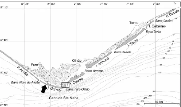
Figure 2.1 – Location of the two sampling stations in the Ria Formosa coastal
lagoon (image adapted from Barbosa. 2006). The arrow indicates the inner station and the rectangle the outer station.
12
Figure 2.2 – Schematic representation of experimental treatments with different
proportions of diluent (white) and sample (blue). The four different sample dilutions were (A) +0.10, (B) +0.25, (C) +0.50, (D) +1.00 and (E) -1.00. The (+) means enriched with nutrients and the (-) means no addition of nutrients (from Barbosa & Domingues, 2009).
14
Chapter 3
Figure 3.1 – Chlorophyll a concentration with the standard error in the two
station of Ria Formosa at the sampling day. NA: not available. 23
Figure 3.2 – (A) Annual percentage of phytoplankton group specific in the
inner station of Ria Formosa at the sampling day. (B) Annual percentage of phagotrophic protists in the inner station of Ria Formosa at the sampling day.
25
Figure 3.3 – (A) Annual percentage of phytoplankton group specific in the
outer station of Ria Formosa at the sampling day. (B) Annual percentage of phagotrophic protists in the outer station of Ria Formosa at the sampling day.
26
Figure 3.4 – (A) Apparent growth rate of phytoplankton community and
dilution factors in the inner zone of the Ria Formosa in spring 2015. (B) Apparent growth rate of phytoplankton community and dilution factors in the outer zone of the Ria Formosa in spring 2015. The open circles represent data that was not used to adjust the regression lines.
28
Figure 3.5 – (A) Apparent growth rate of phytoplankton community and
dilution factors in the inner zone of the Ria Formosa in autumn 2015. (B) Apparent growth rate of phytoplankton community and dilution factors in the outer zone of the Ria Formosa in autumn 2015.
30
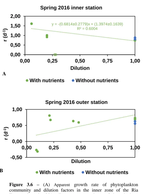
Figure 3.6 – (A) Apparent growth rate of phytoplankton community and
dilution factors in the inner zone of the Ria Formosa in spring 2016. (B) Apparent growth rate of phytoplankton community and dilution factors in the outer zone of the Ria Formosa in spring 2016.
32
Figure 3.7 – (A) Potential instantaneous growth rate of phytoplankton
group-specific in the Ria Formosa in spring 2015. (B) Grazing rate of phytoplankton group-specific in the Ria Formosa in spring 2015. NA: not available.
34
Figure 3.8 – (A) Potential instantaneous growth rate of phytoplankton
group-specific in the Ria Formosa in autumn 2015. (B) Grazing rate of phytoplankton group-specific in the Ria Formosa in autumn 2015. NA: not available.
xi
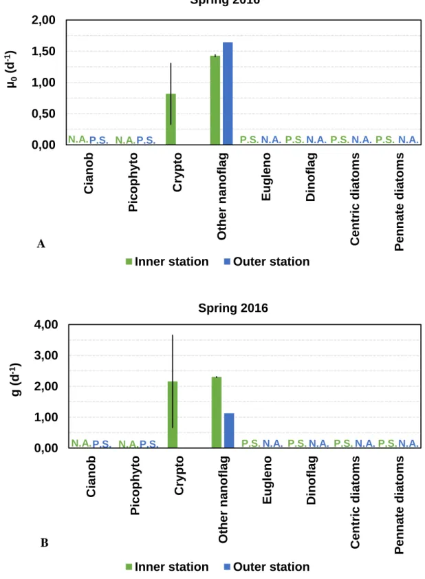
Figure 3.9 – (A) Potential instantaneous growth rate of phytoplankton
group-specific in the Ria Formosa in spring 2016. (B) Grazing rate of phytoplankton group-specific in the Ria Formosa in spring 2016. NA: not available.
38
Figure 3.10 – (A) Microzooplankton growth in the inner station of the Ria
Formosa during spring 2015. (B) Microzooplankton growth in the outer station of the Ria Formosa during spring 2015. NA: not available.
39
Figure 3.11 – (A) Microzooplankton growth in the inner station of the Ria
Formosa during autumn 2015. (B) Microzooplankton growth in the outer station of the Ria Formosa during autumn 2015.
40
Figure 3.12 – (A) Microzooplankton growth in the inner station of the Ria
Formosa during spring 2016. (B) Microzooplankton growth in the outer station of the Ria Formosa during spring 2016. NA: not available.
41
Chapter 4
Figure 4.1 – Five types of responses between the apparent growth of
phytoplankton and dilution factors: (A) insignificant, (B) negative linear, (C) negative saturated, (D) saturated increasing and (E) positive linear (from Dix & Hanisak, 2015).
xii
List of tables
Chapter 3
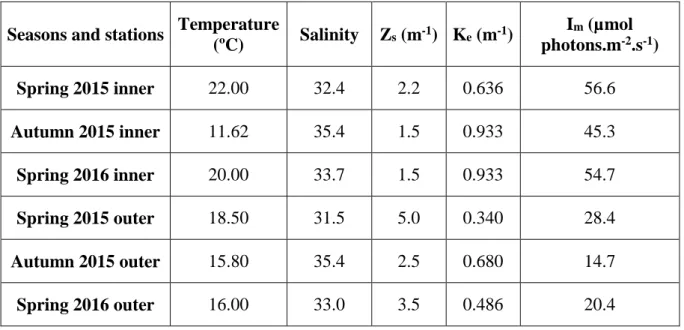
Table 3.1 – Physical and chemical variables in situ and estimated in the two
stations of Ria Formosa at the sampling day. 22
Table 3.2 – Group specific composition of phytoplankton and
microzooplankton and abundance. N.A.: not available. All the numbers must be
multiple by 103 to have the real value (cel.L-1).
xiii
List of abbreviations
Chl a Chlorophyll a
DON Dissolved organic nitrogen
DOP Dissolved organic phosphate
Im Average light intensity in the mixed layer
1
2
1. Introduction
1.1. Phytoplankton
Phytoplankton is a group of prokaryotic and eukaryotic photosynthetic organisms that drift in the water column with the currents (Bidle & Falkowski, 2004; Ajani & Rissik, 2009). Phytoplankton includes Cyanobacteria, diatoms, dinoflagellates, coccolithophore and others flagellates (Ajani & Rissik, 2009). Phytoplankton can also be classified according to cell size, as Picophytoplankton (0.2 to 2.0 µm), Nanophytoplankton (2 to 20 µm) and microphytoplankton (20 to 200 µm). Nevertheless, some taxa attain up to 4000 µm (Ajani & Rissik, 2009). Cell dimensions are relevant because they control, directly and indirectly, the pathways and efficiencies of energy transfer from primary producers to consumers (aquatic food webs), including those sustaining upper trophic levels (Cloern & Dufford, 2005). This microscopic algae have many distinct biochemical contents (Cloern & Dufford, 2005), thus they can be organized into functional groups, pico-autotrophs, nitrogen-fixers, calcifiers, silicifiers and dimethyl sulfide (DMS) producers (Nair et al., 2008).
Phytoplankton is the main primary producer of marine ecosystems, that is, the producers of autochthonous organic material that will fuel aquatic food webs. However, they are as well important to the Earth’s primary production, because phytoplankton can fix about 50 Gt of carbon per year, as much as the tropical rainforests, thus representing almost half of global primary production of the planet (Falkowski et al., 2004). So, phytoplankton is a key player for aquatic systems’ functioning. Besides this function, phytoplankton has significant impacts on water quality and play vital roles in many ecosystem processes, such as in biogeochemical processes, mediating cycling, sequestration and exportation of inorganic and organic compounds. Moreover, phytoplankton is an excellent model systems to address fundamental ecological questions (Litchman & Klausmeier, 2008; Pereira Coutinho et al., 2012), and paleoenvironmental reconstructions (Barbosa, 2009). Then this planktonic group plays a key role in regulating the ecological conditions and changes, and can be used to understand and predict the functioning and production of aquatic ecosystems and the possible responses to natural and anthropogenic-induced changes (Cloern & Dufford, 2005; Smetacek & Cloern, 2008).
3 Even though phytoplankton is biologically and functionally very diverse, it is regulated in the same way, by environmental factors that regulate phytoplankton growth (bottom-up regulation) or phytoplankton loss (top-down regulation). However, it is also affected by anthropogenic activities, such as eutrophication and climate change. Thus the spatial and temporal variability of phytoplankton in aquatic ecosystems reflects the interaction between abiotic and biotic factors (Domingues, 2010).
Bottom-up regulation of phytoplankton includes the effects of resources that control cell replication, such as nutrients, light, temperature, pH, salinity and oxygen concentration, and phytoplankton cells compete among each other for these resources (Domingues, 2010). Nutrients are usually considered the most important factor regulating phytoplankton growth, because they are essential for cell growth, some in relatively large amounts, the macronutrients (e.g., C, H, O, N, P, Si, Mg, K, Ca), and others in much smaller quantities, the micronutrients or trace elements (e.g., Fe, Mn, Cu, Zn, Ba, Na, Mo, Cl, V, Co) (Parsons et al., 1984). Most of these elements are available in sufficient amounts in marine and freshwaters, but others, particularly nitrogen (N), phosphorus (P) and silicon (Si, required only by Si-containing cells such as diatoms), may occur in natural waters in extremely low concentrations for phytoplankton growth. Therefore, these elements, which are taken up by cells mostly in their inorganic form, will often limit phytoplankton growth (Parsons et al., 1984; Domingues, 2010).
Top-down regulation of phytoplankton involves mortality and other loss processes that decrease the number of phytoplankton cells by mortality or removal (Reynolds, 1997). These processes include grazing, cell lyses, viral lyses, cell apoptosis, advection and sinking. Grazing by phagotrophic protists (microzooplankton) are considered the major mortality source of phytoplankton in the oceans (Calbet & Landry, 2004).
1.2. Microzooplankton
Microzooplankton is a group of heterotrophic and mixotrophic organisms that attain up to 200 µm. Includes protists (e.g., ciliates), dinoflagellates and ameboid forms (e.g., foraminifera), small metazoans (e.g., copepods nauplii), and some meroplanktonic larvae (Redden et al., 2009).
4 Usually, microzooplankton is classified as a primary consumer (herbivore), because these organisms occupy a key position in marine food webs as large consumers of primary production (Calbet & Landry, 2004), consuming, on average, 62% of the daily production of phytoplankton (Schmoker et al., 2013), is an important link between primary producers and higher trophic levels (e.g. copepods) in sub-polar and polar waters as well as in temperate and tropical waters (Levinsen & Nielsen, 2002; Calbet & Saiz, 2005; Campbell et al., 2009; Sherr et al., 2013), and as key components of the microbial loop (Sherr & Sherr, 2002).
The temporal variability of microzooplankton herbivory can determine the onset, duration and termination of phytoplankton blooms, sometimes dominated by relatively large and/or toxic cells (Sautour et al., 2000; Strom et al., 2001; Calbet et al., 2003; Odate & Imai, 2003; Clough & Strom, 2005; Sun et al., 2013).
1.3. Techniques for measuring microzooplankton grazing
The impact of the microzooplankton grazing on marine phytoplankton started to be measured through an indirect estimation, from production budgets of phytoplankton (Riley, 1956) and energetic requirements of organisms based on their size (Beers & Stewart, 1971). Then the direct estimations were developed, like the extrapolation from laboratory-determined feeding relationships to field situations of known species abundance of microzooplankton and size composition of potential prey (Heinbokel & Beers, 1979). However, this approach is only viable in cases of well-known feeding rates, behavior and prey preferences, and the available data is not extensive neither accurate, therefore the method is laborious and unsuited for the estimation of total microzooplankton impact on phytoplankton (Landry & Hassett, 1982).
A more direct technique was presented by Capriulo and Carpenter (1980), where the natural assemblage of plankton is divided into two size components, one fraction contains a few microzooplankton, but the majority is their preferred food and serves as a control, and the other fraction contains only plankton with more than 35 µm. Then grazing rates are measured, relative to the control, in a mixture of the smaller and larger size fractions. Nevertheless, this method has two limitations, one is that phytoplankton abundance and size composition differ between experimental and control containers,
5 thus the interpretation of grazing impact from general measures of phytoplankton biomass is ambiguous. The second is that the technique measures grazing impact only for the microzooplankton community bigger than 35 µm (Landry & Hassett, 1982).
According to Landry and Hassett (1982), the techniques developed until then to determine the grazing exerted by microzooplankton were problematic. Therefore they developed a new technique to estimate the herbivory by microzooplankton in natural seawater communities, the dilution method. This approach is the most commonly used, and is a useful method to assess the microzooplankton grazing impact and phytoplankton growth rates (Strom et al., 2001; Moigis & Gocke, 2003; Calbet & Landry, 2004; McManus et al., 2006; Paterson et al., 2007 and 2008).
This technique consists in the manipulation of the encounter rates between phytoplankton and their microzooplankton grazers through a series of different dilutions, which is prepared using particle-free water from the same source, to estimate potential and in situ instantaneous growth rate of phytoplankton, and grazing rate exerted by microzooplankton (Landry & Hassett, 1982).
Also the changes in phytoplankton abundance can be determined by the instantaneous coefficients of population growth and mortality by predation. This is a common assumption in most studies when regarding grazing of phytoplankton. Taking this information into account, it is expected to obtain an inverse relationship between the dilution factor and the growth rate of phytoplankton. This inverse relationship will generate a negative slope, which is the predation coefficient.
The approach relies on three basic assumptions concerning the nutrients, phytoplankton and microzooplankton. The first states that individual phytoplankton growth rate is limited neither by density dependent nor by nutrients during the course of the experiment, which implies that instantaneous growth rate of the prey community is assumed to remain constant throughout the dilution series. For that reason, in the dilution series, nutrients were added in the samples to compare and to correct for nutrient-replete growth rates. The second assumes that phytoplankton grow is exponential. The third assumption arrogates that the probability of a phytoplankton cell being consumed is directly related to the rate of contact between consumers and preys.
6 This means that consumers are not saturated with natural density of prey and the number of prey ingested by a particular consumer is linearly related to prey density (Landry & Hassett, 1982). Other implication is that grazer abundance relative to dilution level does not change over the incubation period (Dix & Hanisak, 2015).
The advantages of the dilution method are that is a simple method and requires little manipulation of the natural communities, except the dilution itself and the addition of nutrients to satisfy the assumption that the phytoplankton growth rate is not limited by nutrients nor by density dependence (Dolan et al., 2000). Furthermore, with the development of this technique it was possible the determination of the phytoplankton saturation, this is when grazing by microzooplankton becomes irrelevant (Redden et al., 2002). Another possible study is the observation of specific mortality of phytoplankton by grazing. In studies of Obayashi and Tanoue (2002), it was found that the microzooplankton has a preference for green microalgae.
Since its introduction, the dilution technique has been widely applied and used in combination with taxon-specific pigment analysis by high-performance liquid chromatography (HPLC) (e.g. Burkill et al., 1987; Latasa et al., 1997; Landry et al., 1998; Obayashi & Tanoue, 2002; Selph et al., 2011) and with flow cytometry (e.g. Landry et al., 1995a; Kuipers & Witte, 2000; Liu et al., 2002; Selph et al., 2011). Both combinations can provide growth and mortality rates associated with specific groups of phytoplankton, which allows the understanding of trophic interactions in complex food webs and subsequent carbon dynamics. However in this study, neither combination was used.
1.4. Ria Formosa: processes and plankton
The Ria Formosa is a shallow coastal lagoon system (Andrade et al., 2004; MCOA, 2008), located at the interface between land and sea, consequently is influenced by different factors that affect the primary productivity of these systems, such as nutrients inputs (Brito et al., 2010). Shallow coastal lagoons are dynamic and highly valuable systems in the land-sea interface, and normally have a strong salinity range from salty to brackish waters, depending on the freshwater inputs and the level of water exchange with the sea (Kjerfve et al., 1996). There are occasions when lagoons have hypersaline
7 waters due to evaporation, which is very common in systems such as Ria Formosa (Kjerffve et al., 1996; Brito et al., 2010).
Given the dynamic conditions of the coastal lagoons, especially in terms of the physical characteristics and salinity regime, the number of species present in these lagoons is very restricted when compared to more stable habitats, such as the marine habitats (Joint Nature Conservation Committee: JNCC; Pecqueur et al., 2011). This kind of habitat can provide valuable ecosystem services and, in conjugation with the fact that shallow coastal lagoons are relatively uncommon in Europe, justify the classification of coastal lagoons as priority habitats in the European Union (Gönenç and Wolfin, 2005).
Ria Formosa is a very productive ecosystem (Santos et al., 2004; Newton & Icely,
2006; Cunha & Duarte, 2007), with an average primary production of ~1400 g C m-2.yr
-1 (Sprung et al., 2001), and the phytoplankton is the main contributor to this mean
(Duarte et al., 2008). Due to its high productivity, this lagoon system can provide many ecological, (e.g. a breeding, wintering and staging area for various species of water birds and nursery for aquatic species), economical (e.g. nursery for aquatic commercial species like cephalopods, fishes, crustaceans and bivalves, aquaculture and salt extraction) and cultural (e.g. esthetic value for tourism) goods and services (MCOA, 2008; Ribeiro et al., 2008; Anthony et al., 2009; Barbosa, 2010; Brito et al., 2010).
The multiple services which Ria Formosa can offer, allows an increase of urban development, tourism and agriculture, and that can lead to a deterioration of the water quality (decreased oxygen saturation, increased concentration of fecal coliform and others, and increased organic matter) and eutrophication (increased concentration of dissolved inorganic nutrients in the water column), due to the discharge of untreated or partially treated domestic and industrial sewage, and agricultural runoff (Dionísio et al., 2000; Newton et al., 2003; Newton & Mudge, 2003; Santos et al., 2004; Mudge et al., 2007; Mudge et al., 2008; Cabaço et al., 2008). However, the status of this lagoon system can vary from “bad” to “good” depending on the criteria. Based on the European Environmental Agency (nutrients concentration) has a “poor” to “bad” status, but according with the United States Estuarine Eutrophication Assessment has a “good” status (Newton et al., 2003). Other two criteria to classify the status of the lagoon is
8 with the diversity of benthic macrofauna and the dissolved oxygen, and to have a “good” status, they have to be high (Gamito, 2008; Newton et al., 2009).
The processes that reduce the abundance of phytoplankton in the Ria Formosa include pelagic and benthic predation and exportation with tidal currents. However, predation by microzooplankton is the main source of mortality of phytoplankton, and their impact is more significant for the Eukaryote Picophytoplankton and Plastidic Nanoflagellates (Barbosa, 2006). When this reduction processes fails, and there is no limitation of nutrients, it may occur a harmful algal bloom (HAB). Which will increase the toxins concentration in the water column, and consequently the capture of bivalves will be prohibited, because the intake of contaminated bivalves can cause serious health problems (FAO, 2011).
Despite the relevance, there are only two studies addressing microbial trophic dynamics, including phytoplankton herbivory, in the Ria Formosa: Thiele-Gliesche (1992) and Barbosa (2006). Other studies addressing phytoplankton in the Ria Formosa were regarding the stressed spatial and seasonal variability of phytoplankton composition, biomass and production (Loureiro et al., 2006), the influence of nutrient enrichment (Falcão & Vale, 2003; Edwards et al., 2005; Loureiro et al., 2005; Newton & Mudge, 2005) and the phytoplankton growth and microzooplankton grazing under increased temperature (Barreto, 2012).
1.5. Study objectives
The objectives of this study were to determine the phytoplankton group-specific growth and grazing rates and the grazing impact of microzooplankton on phytoplankton in the Ria Formosa coastal lagoon, a protected coastal ecosystem. In order to have a better analysis of the trophic dynamics in Ria Formosa, it were chosen two distinct zones, an inner zone of the lagoon system and outer zone, and two different seasons, spring and autumn. What makes these zones so distinct are their locations, one is more protected while the other is not, and is therefore more influenced by the adjacent coastal zone. This factor will change the biotic and abiotic conditions between seasons. For the seasons, only spring and autumn were chosen because the study period was not
9 sufficient for an annual study but also because these seasons are distinct periods of time, excellent for seasonal comparison. The method used was the dilution technique.
10
11
2. Materials and Methods
2.1. Study area
The Ria Formosa is located on the south coast of Portugal and extends approximately 55 km from east to west, and 6 km from north to south, and has an average depth of 2 m (Andrade et al., 2004; MCOA, 2008). It is characterized by a semi-closed aquatic ecosystem with a semi-diurnal tidal regime and a mesotidal system of multiple water inlets, thus being very dynamic, and is partially separated by barriers Ocean Islands (Newton & Mudge, 2003; Barbosa, 2010). This coastal lagoon is considered priority area for conservation within the international legislation, being part of the Ramsar and the Natura 2000 European conservation networks (Ramsar; European Comission).
The climate of the study area is Mediterranean, with wet winters and hot dry summers. The atmospheric temperature varies between 8°C and 30°C, with average values between 16ºC and 20ºC. The annual insolation ranges between 3000 and 3200 hours, while the precipitation is concentrated from November to February, ranging between 400 and 600 mm (Serpa et al., 2005). This ecosystem is in a region that was classified by the Intergovernmental Panel on Climate Change (IPCC, 2007) as being very vulnerable to climate change.
The Ria Formosa is one of the most important and vulnerable ecosystems in Portugal (Domingues et al., 2015), and it is strongly subjected to anthropogenic activities and natural nutrient inputs. The various anthropogenic factors are urbanization, intensive agriculture, aquaculture and coastal engineering (Newton et al., 2003). The natural nutrient inputs are due to regular upwelling events that occur in the coastal area adjacent to the lagoon system, and which influence the outer area of the Ria Formosa and may extend to the inland areas. These events are most often between March and October (Loureiro et al., 2006; Relvas et al., 2007; Barbosa, 2010; Cravo et al., 2014).
12
2.2. Sampling strategy
Sampling was conducted between May 2015 and May 2016, and two stations were sampled: an inner zone and an outer zone (see Fig.2.1). The inner station is located in a confined area of the western sector of the Ria Formosa (Faro beach), has an average depth of 2.5 m and is located in an area of subtidal stands of Cymodocea nodosa. The outer station is located at the main inlet (Barra Faro-Olhão), next to the navigation buoy nº 2, in contact with the adjacent coastal zone and presents an average depth of 15 m. The samples were collected in different tidal stages ebb-tide for the inner station and flood-tide for the outer station.
Figure 2.1 – Location of the two sampling stations in the Ria Formosa coastal lagoon (image
adapted from Barbosa. 2006). The arrow indicates the inner station and the rectangle the outer station.
The Ria Formosa has a reduced depth and has an absence of stratification of the water column (Benoliel, 1984, 1985, 1989; Newton & Mudge, 2003), so the samples were collected only at the surface level, about 10 cm from the surface. Water samples were collected with the aid of a plastic collector of 5 L, previously washed 3 times with water from the station, sealed and transported to the laboratory. During the transportation, the bottles were protected from the sun light and turbulence. For each sampling, in situ water temperature and salinity were measured with a multiparameter sensor and the
13 Secchi depth was measured for subsequent determination of the average photosynthetic
active radiation (PAR) light intensity in the mixed layer (Im).
The Im was considered as a percentage of the light intensity in the surface (I0), using
values of the mixed layer depth (Zm) and the vertical light extinction coefficient (Ke), as
the equation 1 (Kirk, 1986). So, for the outer station it was used the equation 2
(non-turbid, Zs > 5 m; Poole & Atkins, 1929) and for the inner station was the equation 3
(turbid aquatic systems, Zs < 5 m; Holmes, 1970), because the stations have different
values of turbidity. Im= (I0× (1 − e−Ke×Zm)) × ( 1 Ke× Zm) Equation 1 Ke = 1.7 Zs Equation 2 Ke = 1.4 Zs Equation 3 Where:
I0 – PAR intensity at the surface (units: µmol photons.m-2.s-1)
Im – Average light intensity in the mixed layer (units: µmol photons.m-2.s-1)
Ke – Vertical light extinction coefficient (units: m-1)
Zm – Mixed layer depth (units: m-1)
Zs – Secchi disk depth (units: m-1)
2.3. Experimental design: dilution method
The entire procedure was performed under low light conditions. Two different methods of filtration were used to prepare particle-free water (diluent), Whatman GF/F glass fiber filters with a pore of 0.7 µm and a cartridge. Four different sample dilutions were prepared (Dil. 0.10, 0.25, 0.50 and 1.0) in 10 L Thermo Scientific Nalgene bottles, and in order to avoid differences in nutrient concentration among dilutions during the experiment, the treatments were enriched with inorganic macronutrients (+5 µM of
14
orthophosphate (PO43-)). In a second set of samples, nutrients were not added to allow
the analysis of the significance of them.
After the homogenization of the experimental treatments (sample dilutions), they were transferred to duplicate 2L polycarbonate bottles (see Fig.2.2), and sealed with parafilm. The bottles were placed randomly inside an incubation tank in a vertical position. The tank was placed outside the laboratory so it could be under natural insolation conditions, and was covered with nets, to simulate the average light intensity in the mixed layer (see equation 1), creating conditions similar to in situ. The incubation period was 24 hours. All water aliquots were drawn from a well-mixed carboy, including samples for initial concentrations of chlorophyll and microorganisms abundances.
Figure 2.2 – Schematic representation of experimental treatments with different proportions of diluent
(white) and sample (blue). The four different sample dilutions were (A) +0.10, (B) +0.25, (C) +0.50, (D) +1.00 and (E) -1.00. The (+) means enriched with nutrients and the (-) means no addition of nutrients (from Barbosa & Domingues, 2009).
2.4. Quantification of phytoplankton and microzooplankton 2.4.1. Chlorophyll a concentration
Chlorophyll a concentration (Chl a), as indicator of the total phytoplankton biomass, in
all experimental treatments, at the beginning (t0) and at the end of the incubation period
(t24), was analyzed using two methods, a semi-quantitative (Chl a in vivo fluorescence)
and a quantitative (extracted Chl a). Chl a in vivo fluorescence was evaluated using a fluorimeter 10-AU-005-CE of Turner Designs Instruments and was analyzed only to have an estimation of the Chl a concentration. To quantify the Chl a concentration it was used the Lorenzen (1966) method. After sample filtration through a Whatman GF/F glass fiber filters (0.7 µm pore), filters were macerated with 5 mL of acetone 90%, then more 5 mL were added, and stored in a refrigerator. After 24 hours, the samples were centrifuged and analyzed in a fluorimeter, 10-AU-005-CE of Turner Designs
15 Instruments, before and after the addition of hydrochloric acid (HCl) to correct for phaeopigments. These pigments are Chl a degradation products, which are indicators of grazing activity (Jeffrey, 1980). To determined Chl a concentration it was used the equation 4 (see JGOFS, 1994).
𝐶ℎ𝑙 𝑎 (µ𝑔. 𝐿−1) = ( 𝐹𝑚 𝐹𝑚− 1) × (𝐹0− 𝐹𝑎) × 𝐾𝑥× ( 𝑉𝑜𝑙𝑒𝑥 𝑉𝑜𝑙𝑓𝑖𝑙𝑡) Equation 4 Where: Fm – Acidification coefficient
F0 – Reading before acidification
Fa – Reading after acidification
Kx – Door factor from calibration calculations
Volex – Extraction volume
Volfilt – sample volume
2.4.2. Abundance and composition of phytoplankton and microzooplankton
It was taken two subsamples, before and after incubation period, then it was added the fixers, glutaraldehyde solution (final concentration of 1%) in one subsample, and lugol solution (0.3 mL per 100 mL of sample) in the other. The samples with glutaraldehyde solution were stored in dark glass bottles and placed in a refrigerator, while the ones with lugol solution were stored in plastic bottles and in the dark.
Afterwards, it was proceeded the preparation of the samples, with glutaraldehyde, to identify and quantify the abundance of Picophytoplankton, nanophytoplankton and phagotrophic nanoprotists (zooplankton) using the epifluorescence microscope of Zeiss Axio Observer.A1, with the addition of proflavine (20 µL per 1 mL of sample). This preparation had to be performed until 24h after the fixation of the sample.
The filters used were a cellulose acetate with 0.4 µm of pore (support filter to ensure homogeneous distribution), and a black polycarbonate membrane with 0.4 µm of pore. It was pipetted a given volume of sample, proflavine was added, and waited 3 min. Completing this period, the sample with proflavine was filtered with a pressure lower
16 than 100 mm, in order to minimize damage or loss of cells. It was placed into a slide a non-fluorescent oil drop, followed by the polycarbonate membrane which contained the cells, an extra non-fluorescent oil drop and a coverslip (Haas, 1982). The obtained preparations were stored into the freezer for later observation. During the observation, the phytoplankton was integrated into the following groups, Cyanobacteria
Synechococcus, Eukaryotic Picophytoplankton and Plastidic Nanoflagellates, while the
phagotrophic protists were into Aplastidic Nanoflagellates.
As for the samples with lugol solution, a known volume was settled in a sedimentation column (graduated cylinders) for 72h (4h per 1 cm). During the observation it was analyzed the microphytoplankton, such as plastidic dinoflagellates and diatoms, and the microphagotrophic protists (zooplankton), such as ciliates and aplastidic dinoflagellates, on the inverted microscope of Zeiss Axio Observer.A1(Sournia, 1978).
Both in epifluorescence and inverted microscopy were counted at least 400 cells in total, to have only 10 % error (Sournia, 1978). To identify the planktonic organisms it were used different identification books and websites. Phytoplankton was identified according to the Swedish Meteorological and Hydrological Institute (SMHI), and Dodge (1982). Microzooplankton was identify through an online guide from Strüder-Kypke et at., Corliss (1979 and 1985), Dodge (1982), and Margulis et al. (1993).
To calculate the abundance of each of phytoplankton and microzooplankton species/group it was necessary different equations, one for the epifluorescence microscope (see equation 5) and another for the inverted microscope (see equation 6).
𝐴𝑏𝑢𝑛𝑑𝑎𝑛𝑐𝑒 (𝑐𝑒𝑙. 𝐿−1) =𝑋 × 𝐴 × 𝑑
𝑎 × 𝑛 × 𝑉 Equation 5
Where:
X – Total number of enumerated cells
A – Area of the polycarbonate filter (mm2)
d – Correction factor for sample dilution induced by the preservative
a – Area of field observed (mm2)
17 V – Volume of the filtered preserved sample (L)
𝐴𝑏𝑢𝑛𝑑𝑎𝑛𝑐𝑒 (𝑐𝑒𝑙. 𝐿−1) =𝑋 × 𝐴 × 𝑑
𝑉 × 𝑛 × 𝑎 Equation 6
Where:
X – Total number of enumerated cells
A – Area of the sedimentation chamber (mm2)
d – Correction factor due to sample dilution by the preservative V – Volume of the sedimented fixed sample (L)
n – Number of observed microscopic fields
a – Area of the microscopic field (mm2)
2.5. Phytoplankton community and group-specific growth rate, microzooplankton grazing
The exact dilution factors were estimated based on the in vivo fluorescence of Chl a obtained at the beginning of the experiments (IVF0 observed). The apparent growth rate of phytoplankton community for each experimental treatment and replicate was determined assuming that the growth is exponential, as in equation 7. An identic strategy, based on abundance, was used to calculate the specific rates.
r =ln 𝐼𝑉𝐹24− ln 𝐼𝑉𝐹0
𝑡 Equation 7
Where:
IVF24 – In vivo fluorescence of Chl a at the end of the incubation period
IVF0 – In vivo fluorescence of Chl a at the beginning of the incubation period
t – Incubation period (1 day)
A scatter plot was generated using the exact dilution factor represented on the x-axis, and the apparent growth rate of phytoplankton (r) in the y-axis, and alinear regression line was adjusted for each data set (sample, date and/or phytoplankton taxa). On the scatter plot it were used both set of samples, with and without nutrients. The potential
18
instantaneous growth rate of phytoplankton (µ0) and microzooplankton grazing rates (g)
were estimated as the regression intercept and regression slope, respectively.
The in situ instantaneous growth rate of phytoplankton (µis) of phytoplankton was
determined according to the equation 8.
𝜇𝑖𝑠= 𝜇0− (𝑟𝐷𝑖𝑙.1.0+− 𝑟𝐷𝑖𝑙.1.0−) Equation 8
Where:
µ0 – Potential Instantaneous growth rate of phytoplankton (after nutrient addition; d-1)
rDil.1.0+ – Apparent growth rate of phytoplankton in the non-diluted sample with nutrients
rDil.1.0- – Apparent growth rate of phytoplankton in the non-diluted sample without nutrients
Net primary production of phytoplankton (NPP) was calculated according to equation 9.
Phytoplankton biomass (B0) was estimated using Chl a in non-manipulated samples
assuming an C:Chl a ratio of 49 mg C for both the inner station and outer station (Barbosa, 2006; Domingues et al., 2008).
𝑁𝑃𝑃(𝜇𝑔𝐶. 𝐿−1. 𝑑−1) = 𝐵
0× (𝑒𝜇×𝑡− 1) Equation 9
Where:
B0 – Phytoplankton biomass in the non-diluted samples (t0; µgC.L-1)
µ – In situ instantaneous growth rate of phytoplankton (d-1)
t – Time (d-1)
The grazing impact of microzooplankton on phytoplankton (I) was estimated as the percentage of the daily production of phytoplankton removed by microzooplankton, in accordance with equation 10.
𝐼 = 100 ×(𝐵0× 𝑒 𝜇𝑡− 𝐵 0) − (𝐵0× 𝑒(𝜇−𝑔)𝑡− 𝐵0) 𝐵0× 𝑒𝜇𝑡− 𝐵0 Equation 10 Where:
B0 – Phytoplankton biomass in the non-diluted samples (t0; µgC.L-1)
19 g – Microzooplankton grazing rate
2.6. Statistical analyses
All the statistical tests and numerical analysis were carried out using statistical program for Windows. The notation for the statistical parameters follows the normally used,
where n is the number of observations, x the average, SE the standard error, R2 the
determination coefficient, F the statistical test of the analysis of variance and p the
probability of a given null hypothesis (H0), rejected for p < 0.05 (Sokal & Rohlf, 1995).
The mean values were presented with the respective standard errors, preceded by the signal ± (x ± SE).
20
21
3. Results
3.1. Initial conditions
3.1.1. Temperature, salinity and water transparency
The water temperature in the inner station, located in the west sector of the lagoon system (Faro beach), between May 2015 and May 2016, varied between 11.62ºC and 22.00ºC. In the outer station, located at the main inlet (Barra Faro-Olhão), in contact with the adjacent coastal region, the values varied between 15.80ºC and 18.50ºC (Table 3.1). Comparing the values of the water temperature between inner and outer station, the inner station had higher values, excepting during the autumn. At the seasonal level, the temperature presented a range of variation between 11.62ºC and 22ºC, with maximum values in the spring.
The salinity in the inner station, between May 2015 and May 2016, varied between 32.4 and 35.4. In the outer station, the values varied between 31.5 and 35.4 (Table 3.1). Comparing the values of salinity between inner and outer station, excepting the autumn, which had no differences, the inner zone during both springs was slightly more saline than the outer zone. At the seasonal level, the salinity presented a range of variation between 31.5 and 35.4, with lower values in periods of rainfall (April and May) and higher values in autumn. The water temperature and salinity correlated negatively and significantly in both seasons (p>0.05).
The values of the Secchi depth (Zs) in the inner station, between May 2015 and May
2016, varied between 1.5 m and 2.2 m. In the outer station, the values varied between 2.5 m and 5.0 m (Table 3.1). These differences were reflected in the values of the
vertical light extinction coefficient (Ke), which can represent the water turbidity, and
presented values between 0.636 m-1 and 0.933 m-1, and 0.340 m-1 and 0.680 m-1,
respectively. Comparing the values, the outer station had higher values of Secchi depth and lower values of water turbidity, while the inner station had the opposite, lower values of Secchi depth and higher values of water turbidity. At the seasonal level, the Secchi depth presented a range of variation between 1.5 m and 5 m, with higher values
during spring, regarding the water turbidity, the values were between 0.340 m-1 and
22
The average light intensity in the mixed layer (Im), which integrated the radiation
incident to the surface, its attenuation velocity in the water column and the depth of the mixed layer, in the inner station, between May 2015 and May 2016, varied between
45.3 µmol photons.m-2.s-1 and 56.6 µmol photons.m-2.s-1. In the outer station, the values
varied between 14.7 µmol photons.m-2.s-1 and 28.4 µmol photons.m-2.s-1 (Table 3.1).
Comparing the values of the average light intensity in the mixed layer between inner and outer station, the inner station had higher values. At the seasonal level, the average light intensity in the mixed layer presented a range of variation between 14.7 µmol
photons.m-2.s-1 and 56.6 µmol photons.m-2.s-1, with higher values during spring.
Table 3.1 – Physical and chemical variables in situ and estimated in the two stations of Ria Formosa at
the sampling day.
3.1.2. Chlorophyll a concentration
The Chl a concentration, obtained with the Lorenzen method, in the inner station,
between May 2015 and May 2016, varied between 0.20 µg.L-1 and 0.76 µg.L-1. In the
outer station, the values varied between 0.14 µg.L-1 and 1.56 µg.L-1. The autumn of
2015 do not have all the data available, due to problems during the experiments (Fig. 3.1). Comparing the values of the Chl a concentration between inner and outer station, there are contradictions, both springs have opposite relations between stations and the values are discrepant. Regarding autumn it is not possible to compare. At the seasonal
level, the Chl a concentration presented a range of variation between 0.14 µg.L-1 and
1.56 µg.L-1, with a maximum value in the outer station during spring 2016.
Seasons and stations Temperature
(ºC) Salinity Zs (m -1) K e (m-1) Im (µmol photons.m-2.s-1) Spring 2015 inner 22.00 32.4 2.2 0.636 56.6 Autumn 2015 inner 11.62 35.4 1.5 0.933 45.3 Spring 2016 inner 20.00 33.7 1.5 0.933 54.7 Spring 2015 outer 18.50 31.5 5.0 0.340 28.4 Autumn 2015 outer 15.80 35.4 2.5 0.680 14.7 Spring 2016 outer 16.00 33.0 3.5 0.486 20.4
23
Figure 3.1 – Chlorophyll a concentration with the standard error in the two
stations of Ria Formosa at the sampling day. NA: not available.
3.1.3. Abundance and composition of phytoplankton and microzooplankton
In the period of time between May 2015 and May 2016, the inner station had an average
abundance of 140.30x10³ ± 300.92x10³ cel.L-1 of phytoplankton and of 103.55x10³ ±
160.26x10³ cel.L-1 of phagotrophic protists. The outer station had an average abundance
of 278.62x10³ ± 428.68x10³ cel.L-1 of phytoplankton and of 188.45x10³ ± 268.33x10³
cel.L-1 of phagotrophic protists. Thus, the outer station had higher abundances; however,
these results are an underestimation since not all the data were available.
The phytoplankton was divided in 8 groups: Cyanobacteria Synechococcus, Eukaryotic Picophytoplankton, Cryptophyceae, Other Plastidic Nanoflagellates, Euglenophyceae, Plastidic Dinoflagellates, Centric Diatoms and Pennate Diatoms. The phagotrophic protists were divided in 3 groups: Aplastidic Nanoflagellates, Ciliates and Aplastidic Dinoflagellates (Table 3.2). Regarding the abundance of these taxonomic and/or morphological groups considered, the Cyanobacteria Synechococcus, Eukaryotic Picophytoplankton, Other Plastidic Nanoflagellates, and Aplastidic Nanoflagellates were higher in the inner station. In the outer station were the same as in the inner station. Comparing the abundances between inner and outer station, it is possible to observe domination, in both, of picoplankton and nanoplankton.
0,0 0,2 0,4 0,6 0,8 1,0 1,2 1,4 1,6 1,8
Spring 2015 Autumn 2015 Spring 2016
Ch lorophy ll a (µ g.L -1) INNER OUTER NA
24
Table 3.2 – Group specific composition of phytoplankton and microzooplankton and abundance. N.A.:
not available. All the numbers must be multiple by 103 to have the real value (cel.L-1).
S p rin g 2016 Ou te r 491 .30 ± 6.22 208 .34 ± 3.11 46 .64 ± 9.33 1436 .59 ± 6.22 N.A . N.A . N.A . N.A . 755 .61 ± 3.11 N.A . N.A . In n er N.A . N.A . 49 .75 ± 1 .55 288 .41 ± 0. 7 8 4 .10 ± 0.15 38 .28 ± 0.30 26 .28 ± 0.15 17 .47 ± 0.46 299 .2 9 ± 0.78 32 .36 ± 0.15 4.25 ± 0.30 Autu m n 2015 Ou te r 1131 .38 ± 5 .26 486 .76 ± 2 .63 28 .94 ± 2 .63 221 .01 ± 5 .26 4 .08 ± 0.10 20 .60 ± 0.10 18 .71 ± 0.20 5 .67 ± 0.30 265 .74 ± 2 .63 23 .88 ± 0.20 14 .43 ± 0.10 In n er 1257 .68 ± 5 .26 544 .64 ± 7 .89 44 .73 ± 2 .63 68 .41 ± 5 .26 6 .07 ± 0.10 26 .87 ± 0.40 15 .03 ± 0.30 9 .45 ± 0.10 447 .29 ± 5 .26 10 .05 ± 0.10 15 .22 ± 0.30 S p rin g 2015 Ou te r N.A . N.A . N.A . N.A . 0.00 44 .5 8 ± 1 .02 26 .29 ± 0.38 8 .38 ± 0. 12 N.A . 46 .08 ± 0. 48 24 .94 ± 0. 21 In n er N.A . N.A . N.A . N.A . 2 .56 ± 0.20 18 .52 ± 0. 39 97 .93 ± 0. 59 9 .26 ± 0.20 N.A . 12 .41 ± 12 .02 7 .49 ± 0.79 Dat e Ph ytopl an k ton C ya noba cter ia Sy ne cho coc cus Euka ryotic P icophytoplankton Cryptophyc ea e Othe r Pl asti dic N anofla ge ll at es Eugle nophyc ea e P lastidi c D inofla ge ll ates C entric D iatoms P enna te D iatoms Ph agotr op h ic prot ists Apla sti dic N anofla g ell ates C il iate s Apla sti dic D inof lage ll ate s
25 The analysis of the annual percentage (May 2015 – May 2016) of each taxonomic and/or morphological group for total phytoplankton and microzooplankton abundance presented the importance of Cyanobacteria Synechococcus (49.8%) and of Aplastidic
Nanoflagellates (90.1%
)
in the inner station (Fig. 3.2A), and of CyanobacteriaSynechococcus (38.8%), Other Plastidic Nanoflagellates (39.7%) and Aplastidic
Nanoflagellates (90.3%) in the outer station (Fig. 3.3B).
Figure 3.2 – (A) Annual percentage of phytoplankton group specific in the
inner station of Ria Formosa at the sampling day. (B) Annual percentage of phagotrophic protists in the inner station of Ria Formosa at the sampling day.
Phytoplankton inner station
Cianob Picophyto Crypto Other P. Nanoflag Eugleno P. Dinoflag Centric Diatoms Pennate Diatoms A
Phagotrophic protists inner station
Ap. Nanoflag Ciliates Ap. Dinoflag B
26
Phytoplankton outer station
Cianob Picophyto Crypto Other P. Nanoflag Eugleno P. Dinoflag Centric Diatoms Pennate Diatoms
Phagotrophic protists outer station
Ap. Nanoflag Ciliates Ap. Dinoflag
Figure 3.3 – (A) Annual percentage of phytoplankton group specific in the
outer station of Ria Formosa at the sampling day. (B) Annual percentage of phagotrophic protists in the outer station of Ria Formosa at the sampling day. A
27
3.2 Final conditions
All the data presented were obtained from the dilution experiments with the cartridge. The dilution obtained from the Whatman GF/F glass fiber filters with a pore of 0.7 µm was less efficient and accurate.
3.2.1. Phytoplankton community growth rate and microzooplankton grazing
The relationship between dilution factors and the apparent growth rate of phytoplankton (r) in spring of 2015 in the inner station had a positive linear regression. So it was impossible to determine the real growth and predation rate, because there were violations of the assumptions (Fig. 3.4A)
The relationship in spring 2015 in the outer zone had a negative linear regression. However, the slope did not have a different value from zero, so it was impossible to determine the real growth and predation rate (Fig. 3.4B). The plots, for both stations, obtain in the experiment without nutrients are in the annex.
28
Figure 3.4 – (A) Apparent growth rate of phytoplankton community and
dilution factors in the inner zone of the Ria Formosa in spring 2015. (B) Apparent growth rate of phytoplankton community and dilution factors in the outer zone of the Ria Formosa in spring 2015. The open circles represent data that was not used to adjust the regression lines.
0,00 0,20 0,40 0,60 0,80 1,00 1,20 0,00 0,25 0,50 0,75 1,00 r (d -1 ) Dilution Spring 2015 inner station
With nutrients Without nutrients A y = -(0.3125±0.1308)x + (0.5376±0.0967) R² = 0.7405 0,00 0,10 0,20 0,30 0,40 0,50 0,60 0,00 0,25 0,50 0,75 1,00 r (d -1) Dilution Spring 2015 outer station
With nutrients Without nutrients B
29 The relationship between dilution factors and the apparent growth rate of phytoplankton in autumn of 2015 in the inner station had a positive linear regression. So it was impossible to determine the real growth and predation rate, because there were violations of the assumptions (Fig. 3.5A).
The relationship in autumn of 2015 in the outer station had a negative linear regression. The slope had a different value from zero, so it was possible to determine the real growth and predation rate. It did not occur nutrients effect, so there were no significant differences between the experiments with and without nutrients (Fig. 3.5B).
In the experiment with nutrients the values of the apparent growth rate of phytoplankton
were between 0.75 d-1 and 3.63 d-1, the predation rate was 3.36 d-1, the potential
instantaneous growth rate was 3.20 d-1, the instantaneous growth rate of phytoplankton
in situ was 3.29 d-1, the net primary production of phytoplankton was 7.96 d-1, and the percentage of daily phytoplankton production removed by microzooplankton was 100.24%. The plots, for both stations, obtain in the experiment without nutrients are in the annex.
30
Figure 3.5 – (A) Apparent growth rate of phytoplankton community and dilution factors in the inner zone of the Ria Formosa in autumn 2015. (B) Apparent growth rate of phytoplankton community and dilution factors in the outer zone of the Ria Formosa in autumn 2015.
-1,50 -1,00 -0,50 0,00 0,50 0,00 0,25 0,50 0,75 1,00 r (d -1) Dilution
Autumn 2015 inner station
With nutrients Without nutrients
y = -(3.3561±0.7236)x + (3.2039±0.3322) R² = 0.8432 0,00 1,00 2,00 3,00 4,00 0,00 0,25 0,50 0,75 1,00 r (d -1) Dilution
Autumn 2015 outer station
With nutrients Without nutrients A
31 The relationship between dilution factors and the apparent growth rate of phytoplankton in spring of 2016 in the inner station had a negative linear regression. The slope had a different value from zero, so it was possible to determine the real growth and predation rate. It did not occur nutrients effect, so there were no significant differences between the experiments with and without nutrients (Fig. 3.6A).
In the experiment with nutrients the values of the apparent growth rate of phytoplankton
were between 0.73 d-1 and 1.61 d-1, the predation rate was 0.68 d-1, the potential
instantaneous growth rate was 1.40 d-1, the instantaneous growth rate of phytoplankton
in situ was 1.48 d-1, the net primary production of phytoplankton was 3.14 d-1, and the percentage of daily phytoplankton production removed by microzooplankton was 63.94%. The plots, for both stations, obtain in the experiment without nutrients are in the annex.
The relationship between dilution factors and the apparent growth rate of phytoplankton in spring of 2016 in the outer station had a positive linear regression. So it was impossible to determine the real growth and predation rate, because there were violations of the assumptions (Fig. 3.6B).
32
Figure 3.6 – (A) Apparent growth rate of phytoplankton
community and dilution factors in the inner zone of the Ria Formosa in spring 2016. (B) Apparent growth rate of phytoplankton community and dilution factors in the outer zone of the Ria Formosa in spring 2016. y = -(0.6814±0.2779)x + (1.3974±0.1639) R² = 0.6004 0,00 0,50 1,00 1,50 2,00 0,00 0,25 0,50 0,75 1,00 r (d -1 ) Dilution Spring 2016 inner station
With nutrients Without nutrients
-0,50 0,00 0,50 1,00 0,00 0,25 0,50 0,75 1,00 r (d -1 ) Dilution
Spring 2016 outer station
With nutrients Without nutrients A