doi: 10.3389/fmars.2020.00670
Edited by: Leonardo Cruz Da Rosa, Federal University of Sergipe, Brazil Reviewed by: Hans Paerl, University of North Carolina at Chapel Hill, United States Natalya D. Gallo, University of California, San Diego, United States *Correspondence: Thomas C. Malone [email protected]
Specialty section: This article was submitted to Marine Biology, a section of the journal Frontiers in Marine Science Received: 04 May 2020 Accepted: 22 July 2020 Published: 17 August 2020 Citation: Malone TC and Newton A (2020) The Globalization of Cultural Eutrophication in the Coastal Ocean: Causes and Consequences. Front. Mar. Sci. 7:670. doi: 10.3389/fmars.2020.00670
The Globalization of Cultural
Eutrophication in the Coastal Ocean:
Causes and Consequences
Thomas C. Malone
1* and Alice Newton
21Horn Point Laboratory, University of Maryland Center for Environmental Science, Cambridge, MD, United States,2Marine Environmental Research Center, University of Algarve, Faro, Portugal
Coastal eutrophication caused by anthropogenic nutrient inputs is one of the greatest
threats to the health of coastal estuarine and marine ecosystems worldwide. Globally,
∼
24% of the anthropogenic N released in coastal watersheds is estimated to reach
coastal ecosystems. Seven contrasting coastal ecosystems subject to a range of riverine
inputs of freshwater and nutrients are compared to better understand and manage
this threat. The following are addressed: (i) impacts of anthropogenic nutrient inputs
on ecosystem services; (ii) how ecosystem traits minimize or amplify these impacts;
(iii) synergies among pressures (nutrient enrichment, over fishing, coastal development,
and climate-driven pressures in particular); and (iv) management of nutrient inputs
to coastal ecosystems. This comparative analysis shows that “trophic status,” when
defined in terms of the level of primary production, is not useful for relating anthropogenic
nutrient loading to impacts. Ranked in terms of the impact of cultural eutrophication,
Chesapeake Bay ranks number one followed by the Baltic Sea, Northern Adriatic Sea,
Northern Gulf of Mexico, Santa Barbara Channel, East China Sea, and the Great Barrier
Reef. The impacts of increases in anthropogenic nutrient loading (e.g., development
of “dead zones,” loss of biologically engineered habitats, and toxic phytoplankton
events) are, and will continue to be, exacerbated by synergies with other pressures,
including over fishing, coastal development and climate-driven increases in sea surface
temperature, acidification and rainfall. With respect to management, reductions in point
source inputs from sewage treatment plants are increasingly successful. However,
controlling inputs from diffuse sources remains a challenging problem. The conclusion
from this analysis is that the severity of coastal eutrophication will likely continue to
increase in the absence of effectively enforced, ecosystem-based management of
both point and diffuse sources of nitrogen and phosphorus. This requires sustained,
integrated research and monitoring, as well as repeated assessments of nutrient loading
and impacts. These must be informed and guided by ongoing collaborations among
scientists, politicians, managers and the public.
INTRODUCTION
During the course of the Twentieth century, increases in
anthropogenic inputs of nitrogen (N) and phosphorus (P) to
coastal ecosystems via river discharge to coastal ecosystems
became the primary cause of eutrophication and consequent
ecosystem degradation in coastal ecosystems worldwide (
Rabalais
et al., 2009, 2010
;
Paerl et al., 2014
), a trend that is arguably
the most widespread anthropogenic threat to the health of
coastal ecosystems (
Rabalais et al., 2009, 2010
;
IPCC, 2014
).
The European Union defines cultural eutrophication as
The
enrichment of water by nutrients, especially compounds of nitrogen
and phosphorus, causing an accelerated growth of algae and higher
forms of plant life to produce an undesirable disturbance to the
water balance of organisms present in the water and to the
quality of the water concerned, (
European Commission, 1991
).
Nixon (1995)
defined eutrophication as
an increase in the rate
of supply of organic matter to an ecosystem and noted that
increases in the supply of organic matter to coastal ecosystems
have various causes, the most common being excess inputs of
labile, inorganic N and P.
Organic matter (OM) in coastal ecosystems is derived from
both autochthonous primary production and allochthonous
inputs from outside the ecosystem. Evidence suggests that the
coastal ocean as a whole has become net autotrophic (primary
production of organic carbon
> respiratory metabolism of
organic carbon) due to increases in anthropogenic inputs of
inorganic nutrients (
Deininger and Frigstad, 2019
). This is
consistent with the conclusion that increases in autochthonous
phytoplankton production are the primary cause of cultural
eutrophication in coastal ecosystems (
Rabalais et al., 2009
;
Bauer
et al., 2013
). Hence, for our purposes, we define the process of
cultural eutrophication as
increases in the supply of organic matter
to an ecosystem that is fueled by anthropogenic inputs of inorganic
nutrients where increases in organic matter are most often due to
excess
1phytoplankton production.
It is generally agreed that N is the primary cause of
eutrophication in most coastal ecosystems
2(
Howarth and
Marino, 2006
;
Paerl, 2018
). During the last half of the twentieth
century, the global supply of dissolved inorganic nitrogen (DIN)
doubled due to anthropogenic activities (
Boyer and Howarth,
2008
;
Beusen et al., 2016
;
Lee et al., 2016
). Anthropogenic inputs
of N into the global environment (160 Tg N yr
−1) now exceed
all natural N-fixation in the ocean (140 Tg N yr
−1) as well
as the proposed
planetary boundary
3of 62 Tg N yr
−1(
Steffen
et al., 2015
). By 2050, the anthropogenic production of DIN is
expected to be ∼ 2 times higher than in the 1990s (
Galloway
et al., 2004
;
Gruber and Galloway, 2008
;
Jickells et al., 2017
).
Thus, we focus on N enrichment as a pressure on ecosystem
states and the resulting changes in ecosystems states as follows: (i)
1“Excess” phytoplankton production occurs when the rate at which organic matter is produced exceeds the capacity of aerobic consumers and physical dilution to prevent accumulations of organic matter.
2This does not mean that phosphorus does not play a role (cf.,Turner and Rabalais,
2013).
3A boundary beyond which human perturbations are predicted to destabilize the Earth’s N cycle on a global scale.
impacts of anthropogenic N enrichment on coastal ecosystems;
(ii) how ecosystem-specific characteristics minimize or amplify
these impacts; (iii) synergies between nutrient enrichment and
other anthropogenic pressures; and (iv) the management of
anthropogenic nutrient inputs and their impacts.
COASTAL ECOSYSTEMS AND SERVICES
Sustainable development depends on healthy ecosystems
that provide four categories of services valued by society
(
Millennium Ecosystem Assessment [MEA], 2005
;
United
Nations Environment Programme [UNEP], 2006
;
Malone et al.,
2014
;
Culhane et al., 2020
):
•
Regulating services (e.g., climate control
4, prevention of
coastal erosion, limiting the extent and impacts of coastal
flooding, and maintenance of water quality);
•
Provisioning services (e.g., supplies of food, raw materials,
and pharmaceuticals;
•
Cultural services (e.g., recreational, aesthetic, and spiritual
benefits); and
•
Supporting services (e.g., presence of critical habitats
5and
biodiversity, primary production of organic nutrients, oxic
conditions, and optimal nutrient cycling) which underpin
the capacity of coastal ecosystems to provide regulating,
provisioning, and cultural services.
Coastal eutrophication threatens the provision of these
services worldwide. Globally, people are concentrated in the
coastal zone (
Small and Cohen, 2004
;
Neumann et al., 2015
)
where the value of ecosystem services is greatest and where
they are most at risk from convergent anthropogenic pressures
(
Halpern et al., 2008
;
Barbier et al., 2011
;
Cooley, 2012
;
Costanza
et al., 2014, 2017
;
Elliff and Kikuchi, 2015
;
Solé and Ariza, 2019
).
Given synergies among these pressures (e.g.,
Rabalais et al.,
2009
;
Newton et al., 2012
;
Bergström et al., 2019
), management
of anthropogenic nutrient enrichment should be implemented
with due consideration of multiple pressures, especially over
fishing (
Worm et al., 2006
), coastal development (
Martínez et al.,
2007
), and climate-driven pressures (
Huntington, 2006
;
Hoegh-Guldberg and Bruno, 2010
).
FRAMEWORK FOR ADDRESSING THE
PROBLEM OF COASTAL
EUTROPHICATION
Cloern (2001)
described the evolution of research on cultural
eutrophication during the twentieth Century (phases I and II)
and articulated a vision for how the problem can become better
understood and managed during the twenty-first Century (phase
III). Phase I focused on anthropogenic nutrient inputs as the
4Assimilation of carbon dioxide and heat from the atmosphere mitigates the impact of anthropogenic carbon emissions.
5For our purposes, critical habitats include both the pelagic habitat and biologically engineered benthic habitats (coral and oyster reefs, seagrass meadows, kelp forests, tidal marshes and mangrove forests).
primary pressure on ecosystems and on the resulting changes in
ecosystem states. Phase II expanded this approach to consider
nutrient inputs in the context of other pressures including coastal
development and over fishing. This underscored the need for
ecosystem-based approaches (EBAs)
6to managing pressures on
ecosystem services (
Imperial and Hennessey, 1996
;
Levin and
Lubchenco, 2008
;
UNESCO, 2012
).
Guided by five questions, Phase III articulates a way forward
for the twenty-first century (
Cloern, 2001
):
(i) How do ecosystem-specific attributes constrain or amplify
the effects of anthropogenic nutrient enrichment on
ecosystem states?
(ii) How does nutrient enrichment interact with other
pressures to alter ecosystem states?
(iii) How are multiple state-changes related to multiple
pressures?
(iv) How do changes in ecosystem states impact the health and
wellbeing of species, including
Homo sapiens?
(v) How can advances in scientific understanding of
eutrophication be applied to manage and mitigate the
effects of multiple anthropogenic pressures?
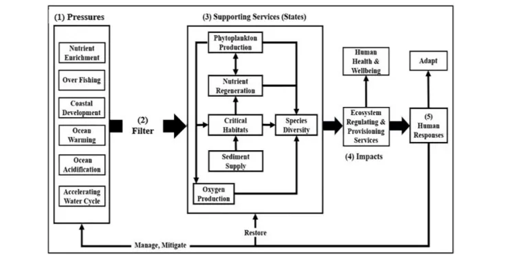
The Driver-Pressure-State-Impact-Response model (
Bowen
and Riley, 2003
;
Niemeijer and de Groot, 2008
;
Elliott et al.,
2017
) provides a framework for understanding the linkages
between drivers (e.g., population growth, industrial agriculture,
and combustion of fossil fuels) that generate pressures, changes
in ecosystem states and services, and human responses to these
changes (Figure 1).
NUTRIENT ENRICHMENT
Global Trends and Patterns
Phytoplankton production is both the foundation of most marine
food webs that support provisioning services and a source of
excess organic matter that often leads to coastal eutrophication.
Today, coastal eutrophication is a global problem (Figure 2),
especially in the northern hemisphere, along the western margins
of the Atlantic and Pacific Oceans, and in European coastal waters
(
Howarth, 2008
;
Nixon, 2009
;
Rabalais et al., 2009, 2010
;
Cloern
and Jassby, 2010
;
Cloern et al., 2014
).
In five years (1998–2003), surface chlorophyll-a (Chl)
7concentration increased by 10% in the coastal ocean (
Gregg et al.,
2005
), largely as a consequence of land-based, anthropogenic
N inputs (
Justi´c et al., 1995
;
Jørgensen and Richardson, 1996
;
IPCC, 2014
). Changes in coastal ecosystem states due to coastal
eutrophication include:
6Ecosystem-based approaches (i) emphasize the protection of ecosystem structure and function; (ii) are place-based; (iii) explicitly account for interactions among species (including humans) and between species and their environment; (iv) consider interactions among ecosystems; and (v) integrate ecological, social, economic, and institutional perspectives.
7An index of phytoplankton biomass.
•
The occurrence of dead zones (hypoxic or anoxic
8)
zones that develop when excess organic matter sinks
below the pycnocline
9where it is metabolized by aerobic,
heterotrophic bacteria (cf.,
Malone et al., 1988
). The
number of oxygen depleted coastal ecosystems has
increased globally from
< 5 prior to WWII to ∼700 today
(
Vaquer-Sunyer and Duarte, 2008
;
Altieri and Diaz, 2019
;
Diaz et al., 2019
), a number that may be an underestimate
due to under sampling of the coastal ocean, especially in the
southern hemisphere (
Altieria et al., 2017
;
Diaz et al., 2019
).
•
Harmful algal blooms
appear to be increasing in
frequency, and there is a growing consensus that cultural
eutrophication is at least partially responsible (
Anderson
et al., 2002
;
Heil et al., 2005
;
Glibert et al., 2008
;
Heisler et al.,
2008
;
Glibert, 2017
;
Glibert and Burford, 2017
).
•
Habitat loss
is a global problem as warm-water coral reefs
have declined by at least 50% (
D’Angelo and Wiedenmann,
2014
;
Hoegh-Guldberg et al., 2017
), seagrass meadows by
29% (
Orth et al., 2006
;
Waycott et al., 2009
;
Deegan et al.,
2012
), and coastal wetlands (mangrove forests and salt
marshes) by 30% (
Valiela et al., 2009
;
Deegan et al., 2012
).
A common theme accompanying these losses is the impact
of anthropogenic nutrient loading.
Sources of Anthropogenic Nitrogen
Over half of the DIN input to coastal ecosystems (including
73% of Large Marine Ecosystems
10) is related to anthropogenic
sources (
Galloway et al., 2004
;
Howarth, 2008
;
Lee et al.,
2016
). An average of ∼20% anthropogenic N inputs to coastal
watersheds is exported to coastal ecosystems (
Howarth et al.,
1996
;
Howarth, 1998
), and
Galloway et al. (2004)
predict that
export will increase by 40–45% by 2050 relative to 2000. Nearly
half of this increase is projected to be from South Asia, where
industrial agriculture and urbanization are expected to show the
greatest increases (
Howarth and Marino, 2006
;
Goldewijk et al.,
2011
;
Lee et al., 2016
). Ranked in terms of the magnitude of N
loading, major
11anthropogenic sources include:
(i) Synthetic Fertilizers
– The largest source of
anthropogenic N transported to coastal ecosystems is the
use of synthetic fertilizers (
Vitousek et al., 1997
;
Johnson
and Harrison, 2015
), which has grown exponentially
from near zero in 1910 to ∼118 × 10
9kg N yr
−1in 2013
(
Penuelas et al., 2013
;
Lu and Tian, 2017
). In 2013, southern
Asia accounted for 71% of global fertilizer use, followed by
North America (11%), Europe (7%), and South America
8Hypoxia, dissolved oxygen concentration ≤ 2 mg liter−1; anoxia, water depleted of dissolved oxygen.
9A rapid increase in density with depth in the water column which separates a vertically mixed surface layer from bottom water.
10The global network of large marine ecosystems (LMEs) includes coastal watersheds and the coastal ocean (estuaries and the open waters of the continental shelves). LMEs vary in size from ∼ 200,000 km−2 to> 1,000,000 km−2 and encompass areas of the coastal ocean where primary productivity is generally higher than in the open ocean (Sherman, 1991).
11In addition to the major sources listed below, there are many, relatively minor, additional sources including industrial sources, especially from biomass and food processing, e.g., paper mills, dairy, brewing.
FIGURE 1 | The framework is conceptualized in terms of (1) anthropogenic pressures on ecosystem support services that (2) are uniquely modulated by each ecosystem as they perturb (3) ecosystem support services (states), changes in which impact (4) regulating and provisioning services. Human responses to these impacts (5) include efforts to manage and mitigate pressures, to restore supporting services, and to adapt to changes in states (modified afterCloern, 2001).
FIGURE 2 | Global distribution of eutrophic coastal marine ecosystems (adapted fromBreitburg et al., 2018). Recent coastal surveys by the United States and the European Union found that 78% of U.S coastal waters and 65% of Europe’s Atlantic coastal waters exhibit symptoms of eutrophication.
(6%) (
Lu and Tian, 2017
). Volatilization of ammonia from
agriculture fields emits an estimated 10 × 10
9kg N yr
−1(8% of the N applied) into the atmosphere (
Vitousek et al.,
1997
;
Bouwman et al., 2013
).
(ii) Combustion of Fossil Fuels
– Emissions from the
combustion of fossil fuels release an estimated 25–40 ×
10
9kg N yr
−1(
Penuelas et al., 2013
) with Asia, Europe,
North America and Sub-Saharan Africa accounting for
30, 20, 17, and 12% of emissions, respectively (
Lamsal
et al., 2011
). As well as being a pressure for eutrophication,
nitrous oxide is a potent greenhouse gas (
Davidson, 2009
).
(iii)
Legume
Agriculture
– Industrial agricultural
has replaced large areas of natural vegetation with
monocultures of legumes (e.g., soybeans) that support
symbiotic N
2-fixing bacteria. As a result, inputs of
N from biological N-fixation to coastal watersheds
has increased from negligible to ∼33 × 10
9kg yr
−1(
Boyer and Howarth, 2008
).
(iv) Animal Husbandry
– The production of manure has
increased rapidly over the last century. Today, agriculture
is responsible for over 75% of the NH
3emissions in
the United States and Canada, with animal production
accounting for
> 70% (
Aneja et al., 2001
;
Bittman
and Mikkelsen, 2009
). Current loads of manure-N are
estimated to be ∼ 18 × 10
9kg N yr
−1, with production
hotspots in western Europe, India, northeastern China, and
southeastern Australia where emissions to the atmosphere
are growing rapidly (
Penuelas et al., 2013
;
Zhang et al.,
2017
).
(v) Wastewater
– Globally, 80% of municipal wastewater
is released into the environment untreated (
World Water
Assessment Programme [WWAP], 2017
). The percentage
of treated sewage varies regionally from 90% in North
America, 66% in Europe, 35% in Asia, 14% in Latin
America and the Caribbean, and
<1% in Africa (
Selman
and Greenhalgh, 2010
). Thus, the most prevalent urban
source of nutrient pressure is human sewage, which is
estimated to have released ∼ 9 ×10
9kg N yr
−1into the
environment in 2018 (extrapolated from
van Drecht et al.,
2009
).
(vi) Finfish aquaculture
– Annual nutrients inputs to the
coastal ocean via finfish aquaculture increased worldwide
by a factor of 6 from ∼ 0.43 × 10
9kg N yr
−1in 1985
to 2.60 × 10
9kg N yr
−1in 2005 (
Strain and Hargrave,
2005
). In contrast, the pressure of nutrient enrichment
from bivalve aquaculture is generally small to negligible.
In fact, bivalve aquaculture is increasingly being used to
offset anthropogenic nutrient pressures (
Burkholder and
Shumway, 2011
;
Gallardi, 2014
).
Globally, nonpoint (diffuse) source inputs (i-iv above) total
∼
200 × 10
9kg N yr
−1and far exceed point source inputs
(v-vi above) of ∼ 10 × 10
9kg N yr
−1or 5% of the total. Thus, our
emphasis here is on inputs from diffuse sources.
Transport Routes
River runoff and atmospheric deposition account for most
anthropogenic N inputs to coastal ecosystems (Figure 3;
Howarth et al., 1996
;
Green et al., 2004
;
Howarth, 2008
;
Jickells
et al., 2017
)
12. During the twentieth Century, total riverine inputs
of N to the coastal ocean increased from ∼27 × 10
9kg N yr
−1 12Ground water discharge is estimated to be< 4% of nutrient exports to coastal waters globally (Beusen et al., 2013). Given this, and challenges of quantifying ground water inputs on regional to global scales (National Research Council [NRC], 2000), this pathway is not considered here.to ∼48 × 10
9kg N yr
−1(
Galloway et al., 2004
;
Beusen et al.,
2016
). Globally, there is a significant linear correlation between
net anthropogenic N inputs to coastal watersheds and total river
borne N export to the coastal ocean (
Boyer and Howarth, 2008
;
Swaney et al., 2012
), and we estimate that ∼24% of anthropogenic
N inputs to coastal watersheds reaches coastal ecosystems.
Anthropogenic inputs of N to the atmosphere are derived
from the volatilization of NH
3from fertilizer and the combustion
of fossil fuels (emission of nitrous oxide). Atmospheric
deposition of N to the global ocean increased rapidly during
the twentieth Century from a pre-industrial rate of ∼ 22 ×
10
9kg N yr
−1to
> 45 × 10
9kg N yr
−1today (
Dentener
et al., 2006
;
Duce et al., 2008
). Of this, it is estimated that
atmospheric deposition directly to the coastal ocean is on the
order of 8 × 10
9kg N yr
−1(
Seitzinger et al., 2010
;
Ngatia et al.,
2019
), or about 14% of total anthropogenic inputs to the coastal
ocean. However, the relative magnitude of direct atmospheric
deposition to coastal ecosystems varies from ∼5% in waters most
heavily impacted by river borne inputs (e.g., the northern Gulf
of Mexico) to ≥ 30% in waters with relatively low river borne
inputs (e.g., Baltic, western Mediterranean, mid-Atlantic and
northeast U.S.-Canadian Atlantic coastal regions) (
Paerl et al.,
2002
;
Spokes and Jickells, 2005
).
PATTERNS AND TRENDS WITHIN
ECOSYSTEMS
For comparative purposes, we have selected a set of coastal
ecosystems that have been impacted by anthropogenic nutrient
loading: three open continental shelf ecosystems (northern Gulf
of Mexico, East China Sea, and the Great Barrier Reef), three
semi-enclosed ecosystems (Baltic Sea, Northern Adriatic Sea,
and Chesapeake Bay), and one eastern boundary upwelling
system (Santa Barbara Channel in the California Current system).
As a group they are subject to a wide range of N inputs
(0.07–2.0 × 10
9kg N yr
−1) and exhibit contrasting capacities
to minimize or amplify the effects of anthropogenic nutrient
enrichment. Sufficient data and information on anthropogenic
nutrient loadings and their impacts for all of these systems have
been collected over long enough periods (decades) to parse major
pressures, impacts and trends. All seven ecosystems exhibit a
range of eutrophic states as indicated by levels of phytoplankton
production
13(Table 1), and, with the exception of the Great
Barrier Reef, all are in the northern hemisphere (Figure 2).
Pressures and Changes in States
Northern Gulf of Mexico (NGM)
The NGM (continental shelf off the states of Louisiana, and
Texas) has an area of ∼60,000 km
2with depths
< 200 m. The
Mississippi-Atchafalaya River system is the primary source of
fresh water (∼80%) and new
14nutrients (∼90%) to the NGM.
13Oligotrophic < 100 g C m−2 yr−1, Mesotrophic 100–300 g C m−2 yr−1, Eutrophic 301–500 g C m−2yr−1, and Hypereutrophic> 500 g C m−2yr−1. 14Nutrients supplied from outside the ecosystem (e.g., nitrate input via upwelling and river runoff) as opposed to nutrients that are regenerated and recycled within the ecosystem (e.g., ammonium).FIGURE 3 | Nutrient enrichment pathways () via river runoff, storm water runoff (Urban and Residential Runoff) and atmospheric precipitation; and effects of anthropogenic nutrient enrichment on phytoplankton biomass (Algal Bloom) and consequences of eutrophication, e.g., oxygen depletion of bottom waters (O2↓) (Source: Hans Paerl, University of North Carolina).
TABLE 1 | Characteristics of the seven ecosystems (NGM – Northern Gulf of Mexico, ECS – East China Sea, GBR – Great Barrier Reef, BS – Baltic Sea, NA – Northern Adriatic Sea, CB – Chesapeake Bay, Santa Barbara Channel – SBC) compared in terms of ecosystem-surface area (×103km2), mean DIN load (109kg N yr−1), mean NPP (g C m−2yr−1), residence time (months), dilution potential (surface area ×1000 ÷ N load), spatial extent of bottom water hypoxia as a percent of ecosystem area, and the frequency of toxic algal events (x – low, xx – moderate, xxx – high).
Area N Load Phytoplankton NPP Residencetime Dilutionpotential Hypoxia Toxic events Rank
NGM 160 1.3 260a 2.5 0.12 25 xx 4 ECS 750 2.0 160b 16 0.37 15 xxx 6 GBR 344 0.08 114c 1 4.30 0 p 7 BS 350 0.64 120d > 360 0.65 19 x 2 NA 19 0.26 140e 5.5 0.07 < 10 xxx 3 CB 12 0.07 320f 7 0.17 40 x 1 SBC 4 0.21 490g 12 0.02 20 xx 5
The systems are ranked in terms of the severity of the effects of eutrophication as indicated by the spatial extent hypoxic bottom water and the frequency of toxic algal events (p = potential occurrence).aBenway and Coble (2014);bLiu et al. (2015);cO’Reilly (2017);Hieronymus et al. (2018);Piontek et al. (2019);eZoppini et al. (1995); Hopkins (1999);Pugnetti et al. (2005, 2006);fHarding et al. (2020);gBrzezinski and Washburn (2011).
Volume transports of the river system range between 220 and
630 km
3yr
−1with a mean of 530 km
3yr
−1(
Aulenbach et al.,
2007
). Depending on river discharge, the spatial extent of the
resulting buoyant, nutrient-rich coastal plume varies from 10,000
to 35,000 km
2with a maximum seasonal extent typically during
May-June5
15. On average, the river-system delivers ∼1.3 × 10
9kg
15 http://mississippiriverdelta.org/files/2018/09/Known-Impacts-of-the-Mississippi-River-1.pdf (Accessed April 21, 2020).N yr
−1(
Dunn, 1996
;
Turner et al., 2007
). Discharge is lowest on
average during September-October and highest during
March-April (
Dunn, 1996
;
Dagg and Breed, 2003
;
Turner et al., 2007
).
Of this input, it is estimated that denitrification and anammox
16remove 40–50% of nitrate inputs annually (
Seitzinger and Giblin,
16Denitrification is generally the dominant pathway for N removal in coastal ecosystems (Dalsgaard et al., 2005).Coastal marine sediments play a critical role in N losses via denitrification and anaerobic ammonium oxidation (anammox).
1996
). Direct atmospheric deposition of DIN to the NGM is small
(
<1%) in comparison (
Goolsby et al., 1999
).
Riverine inputs of nitrate
17have increased by at least threefold
since WW II, with most of this increase occurring between 1970
and 1983 due to increased use of nitrogen fertilizers in the river’s
large watershed (
Goolsby et al., 1999
). Since 1983, annual riverine
inputs of DIN have fluctuated between ∼ 0.6 × 10
9kg yr
−1in
2000 and ∼ 1.8 × 10
9kg yr
−1in 1993. In contrast to N, there
has been relatively little change in P discharge by the Mississippi
over a similar period so that the N:P ratio of the dissolved
nutrient pool is consistently above the Redfield molar ratio of 16
(
Redfield, 1958
).
Phytoplankton biomass is correlated with the riverine supply
of N (
Fennel et al., 2011
), and the annual cycle of phytoplankton
biomass is characterized by a spring maximum and an autumn
minimum (
Bode and Dortch, 1996
;
Gomez et al., 2018
).
Spatially, phytoplankton biomass and NPP vary with salinity
as follows (
Lohrenz et al., 1997, 1999
;
Dagg and Breed, 2003
;
Gomez et al., 2018
):
•
Near
field
(oligohaline)
where
salinity
is
<18,
phytoplankton biomass is ≤5
µg Chl liter
−1, and
phytoplankton NPP is ≤1 g C m
−2d
−1;
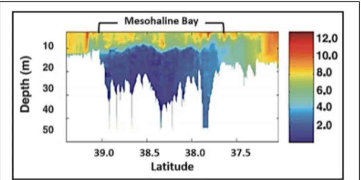
•
Mid
field
(mesohaline)
where
salinity
is
18–32,
phytoplankton biomass is 3–50
µg Chl liter
−1, and
phytoplankton NPP is 0.5–13 g C m
−2d
−1;
•
Far field (polyhaline)
where salinity is
> 32, phytoplankton
biomass is 0.1–10
µg Chl liter
−1, and phytoplankton NPP
is 0.2–3 g C m
−2d
−1).
The spring bloom in the mesohaline fuels the development of
an extensive hypoxic zone that is generally confined to a relatively
thin (1–4 m) bottom boundary layer over the inner shelf from
March to October (
Dagg et al., 2007
;
Justi´c et al., 2007
;
Fennel
and Testa, 2019
). Seasonal hypoxia began expanding in the 1950s
with rapid increases in the time-space extent of hypoxia during
the 1970s (
Rabalais and Turner, 2019
). The spatial extent of
hypoxia over the shelf has varied between
< 5,000 km
2in 2000
and 22,720 km
2in 2017 with a mean of 13,700 km
2making it one
of the largest open shelf hypoxic zone in the world (
Rabalais and
Turner, 2019
; Figure 4). Seasonal hypoxia has resulted in losses
of benthic biodiversity and biomass as longer-lived species are
eliminated (
Committee on Environment and Natural Resources
[CENR], 2000
;
Rabalais and Turner, 2019
).
In addition to bottom water hypoxia, increases in nutrient
loading appears to be promoting the growth of potentially toxic
phytoplankton. The dinoflagellate
Karenia brevis is the primary
toxic species in the NGM where it is ubiquitous at background
levels of
< 1 cell ml
−1(
Steidinger et al., 1998
). Blooms of
K. brevis
(
>10 cells ml
−1) occur almost annually off the west coast of
Florida, but historically have occurred less frequently along the
Texas coast (
Hetland and Campbell, 2007
). The abundance of
Pseudo-nitzschia spp. has increased over the shelf since the
1950s, a trend that may be related to the long-term increase in
nutrient loading (
Dortch et al., 1997
;
Parsons and Dortch, 2002
;
17Human activity preferentially mobilizes nitrate over other forms of nitrogen (Howarth et al., 1996).
Baustian et al., 2016
). Peaks in the abundance of potentially
toxin-producing dinoflagellates (Dinophysis spp. and Prorocentrum
spp.) have been observed to develop in concert with the spring
peak in river flow (
Bargu et al., 2016
).
East China Sea (ECS)
The ECS has an area of ∼750,000 km
2, 75% of which is
< 200
m deep. With a mean volume transport of ∼ 900 km
3yr
−1(
Liu
et al., 2003
), the Changjiang (Yangtze) River accounts for
> 90%
of river runoff and is the largest source of nutrient loadings to
the ECS (
Yan et al., 2010
;
Wu et al., 2011
;
Tong et al., 2015
).
The annual cycle of flow is characterized by a summer maximum
and a winter minimum (
Chen et al., 2016
). Under high summer
flows, the River’s coastal plume spreads eastward over an area that
can cover as much as 30% of the ECS in contrast to the winter
low flow period when the plume is confined to a narrow band
along the coast south of the River’s mouth (
Dong et al., 2010
;
Tong et al., 2015
).
Riverine inputs of N have been increasing since the 1960s
(
Zhou et al., 2008
;
Chen et al., 2019
). Despite the Three Gorges
Dam, which began storing water in 2013, inputs of DIN from
the Changjiang increased by nearly an order of magnitude from
0.220 × 10
9kg N yr
−1in 1970 to 2.0 × 10
9kg N yr
−1in 2012
(
Tong et al., 2015
;
Lin et al., 2017
;
Strokal et al., 2020
). N-fixation
contributes only ∼ 0.013 × 10
9kg N yr
−1or
< 1% of riverine
inputs (
Zhang R. et al., 2012
). Losses of N via denitrification
and anammox are estimated to be equivalent to riverine inputs
of anthropogenic DIN (
Lin et al., 2017
). At the same time,
the dam has reduced the mass transport of suspended matter
and, therefore, the input of P to the ECS (
Xu et al., 2015
).
As a consequence, N:P molar ratios have increased to
>100
(
Huang et al., 2019
).
Dissolved nutrients are also delivered to the ECS by the
Taiwan Warm Current (TWC), the Kuroshio, and atmospheric
deposition (
Chen, 1996, 2008
;
Zhang et al., 2019
). Atmospheric
deposition of N directly to the ECS in 2012 is estimated to have
been ∼80% of riverine inputs. Eutrophication caused by nutrient
inputs from the Changjiang are most pronounced in the near field
plume (salinity
< 30) over the inner shelf (0–50 m) while inputs
from the TWC dominate the mid-field (salinity 31–32) over the
mid-shelf (50–100 m) and inputs from the Kuroshio dominate
the far field (salinity
> 32) over the outer shelf (100–200 m)
(
Wang et al., 2014
). Atmospheric deposition is distributed over
the entire ECS (
Zhang et al., 2019
).
The annual cycle of NPP is characterized by a summer
maximum and a winter minimum. Interannual variations (1998–
2007) in the spatial extent of high Chl are driven by variations in
river discharge (
Xiuren et al., 1988
;
Kim et al., 2009
). Increases
in discharge have led to increases in NPP, increases in the
abundance of small phytoplankton (
<20 µm) and dinoflagellates,
and decreases in diatoms in the coastal plume (
Zhou et al.,
2008
;
Li et al., 2019
). While an interannual trend in Chl for the
ECS as a whole (1996–2014) is not apparent (
O’Reilly, 2017
),
Chl levels in the coastal plume have increased as anthropogenic
nutrient inputs increased while Chl in the far field decreased
due to increases in vertical stratification as the upper ocean
warms (
Kong et al., 2019
). As the plume spreads and mixes with
FIGURE 4 | Mississippi-Atchafalaya River Basin and the frequency (percent occurrence) of mid-summer bottom-water hypoxia off the coast of Louisiana and Texas during 1985–2008 (inset) (Source: Center for Agricultural and Rural Development, Iowa State University).
open shelf water, Chl concentrations decline from high levels
(
>10 mg m
−3) in the plume to low levels (
<0.5 mg m
−3) in
oligotrophic open shelf waters, a pattern that is driven by the
riverine supply of nutrients (
Wang and Wang, 2007
;
Chen, 2008
;
Mackey et al., 2017
).
NPP in the plume is the primary source of particulate
organic matter to the ECS (
Zuo et al., 2016
). As the
Changjiang plume flows over ambient ocean water and the
surface layer warms, the water column becomes increasingly
stratified and this supply of organic matter fuels bacterial
oxygen demand causing bottom waters to become hypoxic
(
Rabouille et al., 2008
;
Liu et al., 2015
;
Wang et al., 2016
;
Zuo et al., 2016
;
Qian et al., 2107
). Persistent summer hypoxia
causes high mortality rates among sessile benthic species and
reduces recruitment to economically important fish populations
(
Levin et al., 2009
).
Hypoxia was first reported in 1959 (
Zhu et al., 2011
).
Interannual increases in NPP has led to increases in the spatial
extent of bottom water hypoxia over the inner shelf from ∼1,800
km
2in 1959 to ∼ 13,700 km
2in 1999 and
> 15,400 km
2in 2006
(
Levin et al., 2009
;
Li et al., 2011
;
Wang et al., 2015
;
Qian et al.,
2107
), a trend that has been attributed to elevated nutrient inputs
due to fertilizer use in the Changjiang watershed (
Wu et al., 2019
).
Bottom water hypoxia now covers
> 15% of the ECS making it
one of the largest coastal hypoxic zones in the world (
Chen et al.,
2007
;
Wang et al., 2016
;
Zhu et al., 2016
).
Intrusions of nutrient-rich oceanic water from the Kuroshio
also contribute to the development of hypoxia. The hypoxic
region north of 30
◦N is dominated by Changjiang inputs,
with its N loads supporting 74% of oxygen consumption; south
of 30
◦N, oceanic nitrogen sources become more important,
supporting 39% of oxygen consumption during the hypoxic
season, but the Changjiang remains the main control on hypoxia
formation also in this region (
Große et al., 2020
). The importance
of oceanic nutrient supply distinguishes hypoxia in the ECS
from the otherwise comparable situation in the NGM, where a
similar spatial extent of hypoxia is fueled by riverine inputs of
anthropogenic nutrients from the Mississippi-Atchafalaya River
system (
Fennel and Testa, 2019
).
In addition to the impacts of hypoxia, increases in the N:P
molar ratio promote blooms of toxic dinoflagellates (
Glibert et al.,
2018
;
Huang et al., 2019
). Reported toxic algal events along the
coast increased from undetected in the 1950s and 60s to 10
in the 70s, 25 in the 80s, and
> 100 in the 90s (
Yan et al.,
2002
). During 2000–2006, the trend continued with most events
occurring during summer (
Yan et al., 2010
) in Zhejiang coastal
waters, particularly in the Zhoushan Archipelago which is home
to the largest marine fishery in China (
Wang and Wu, 2009
).
Particularly, large scale blooms (covering an area
> 1,000 km
2)
have been recorded every year since 1998, and the dinoflagellate
Prorocentrum donghaiense has become the recurrent bloom
species for more than 10 years (
Li et al., 2014
;
Lu et al., 2014
).
Blooms of other potentially toxic dinoflagellates (Karodinium
veneficum, Karenia mikimotoi, K. veneficum, Alexandrium
tamarense, A. catenella, and Heterosigma akashiwo) have also
been observed (
Lu et al., 2014
;
Zhou et al., 2015
;
Wang Y.-F. et al.,
2018
). Toxic dinoflagellate blooms have resulted in millions of
dollars of lost fish landings (
Tang et al., 2006
;
Zhou et al., 2008
;
Li
et al., 2014
;
Mackey et al., 2017
;
Glibert et al., 2018
;
Wang R. et al.,
2018
;
Chen et al., 2019
).
Eutrophication may also be an important factor contributing
to increases in jellyfish abundance and blooms (
Mills, 2001
;
Purcell et al., 2007
;
Diaz and Rosenberg, 2008
;
Richardson et al.,
2009
;
Dong et al., 2010
;
Condon et al., 2011
;
Brotz et al.,
2012
;
Boero et al., 2016
). Three jellyfish species (Aurelia aurita,
Cyanea nozakii, and Nemopilema nomurai) form large blooms,
the frequency of which has been increasing since the 1950s (
Dong
et al., 2010
;
Brotz et al., 2012
).
N. nomurai, the giant jellyfish,
is arguably the most serious threat to fisheries since it is most
abundant in the Changjiang plume where it preys on juvenile fish
(
Sun et al., 2015
).
Great Barrier Reef (GBR)
With a surface area of 344,000 km
2and depths of
< 50 m,
Australia’s GBR is the Earth’s largest reef system. As the reef
developed over the last 20,000 years on the continental shelf,
it formed a large coastal lagoon (
<40 m deep) into which
rivers discharge from 35 watersheds (total mean discharge of 70
km
3yr
−1). Today, rivers are the largest single source of new
nutrients to the lagoon (
Furnas et al., 1997
;
Brodie et al., 2011,
2012
;
Devlin et al., 2015
), and elevated nutrient concentrations
are measurable at distances of hundreds of kilometers from
river mouths (
Devlin and Brodie, 2005
). Riverine inputs are
characterized by episodic peaks in flow with most volume
transport occurring during November–April when large flow
events are most frequent and
> 90% of land-based nutrient inputs
occurs (
Brodie et al., 2011
).
Since European settlement, annual riverine inputs of N and P
to the lagoon have increased from ∼ 0.014 × 10
9kg N yr
−1to
0.080 × 10
9kg N yr
−1and from 1.8 × 10
6kg P yr
−1to 16 ×
10
6kg P yr
−1(
Brodie et al., 2009
;
Kroon et al., 2012
). The form
of N delivered has also changed from predominantly dissolved
organic nitrogen (DON) to predominantly DIN (
Harris, 2001
;
Brodie and Mitchell, 2005
). In addition to riverine inputs,
N-fixation supplies 0.01–0.21 × 10
9kg N y
−1, rainfall 2.7 ×
10
6kg N y
−1, and upwelling 0.001–0.004 × 10
9kg N y
−1(
Furnas et al., 1997, 2011
;
Benthuysen et al., 2016
). Export via
denitrification is estimated to be in the range of 0.016–0.024 ×
10
9kg N y
−1(
Furnas et al., 2011
) or about 25% of total inputs.
Long-term monitoring data show that hard coral cover on the
GBR has reduced by
> 70% over the past century
Bell et al., 2014
).
Waters of the lagoon become progressively more productive as
they flow through the reef system, an increase that is attributed
largely to benthic N-fixation (
Bell et al., 2014
). Current levels
of nutrient enrichment support Chl concentrations that range
from annual means of
< 0.3 µg liter
−1to 0.7
µg liter
−1(
Brodie
et al., 2007
). Under flood conditions during April–November,
peaks in river discharge support phytoplankton blooms in the
central and southern lagoon that yield Chl concentrations of 1–
20
µg liter
−1(
Devlin and Brodie, 2005
;
Devlin and Schaffelke,
2009
;
Brodie et al., 2009, 2010
;
McKinnon et al., 2013
).
Nutrient-driven increases in phytoplankton biomass and macroalgal cover
have been shown to be associated with long term coral reef
decline (
De’ath and Fabricius, 2010
;
D’Angelo and Wiedenmann,
2014
). Clear water
18and low macroalgal cover promote high
coral species richness (
De’ath and Fabricius, 2010
). There is
growing evidence that
Acanthaster planci
19predation events and
coral bleaching are exacerbated by eutrophication and that the
lack of recovery of the reefs is primarily a consequence of high
phytoplankton biomass (
Bell et al., 2014
;
Allen et al., 2019
).
Thus, 23% of the reef system has been degraded in areas with
Chl concentrations
> 0.2 µg liter
−1, concentrations that are
considered to be indicative of eutrophication in the GBR lagoon
(
Bell, 1992
;
Bell et al., 2014
).
De’ath and Fabricius (2010)
predict
that reducing agricultural runoff could reduce macroalgal cover
by 39% and increase the species richness of hard corals and
phototrophic octocorals by 16 and 33%, respectively.
N:P ratios are consistently
< 16 and many processes in
coral reefs are nitrogen limited (
Furnas et al., 2005
), and
18Increases in Chl reduce light penetration. Clear water occurs when the attenuation coefficient for downwelling photosynthetically active radiation is< 0.17.
19The crown-of-thorns (Acanthaster planci) is responsible for the loss of immense stretches of coral throughout the Indo-Pacific region, especially on the GBR. Larvae of this starfish are able to clone themselves, and the frequency of larval cloning increases with increasing phytoplankton biomass. This has the potential to increase the supply of larvae and consequently the abundance of adults (Allen et al., 2019).
increases in river-borne inputs of P have promoted the growth of
Trichodesmium spp. and other N-fixing organisms that introduce
new N into the lagoon-reef system at rates that are far higher now
than in the past (
Bell and Elmetri, 1995
;
Bell et al., 1999
;
Messer
et al., 2017
;
Blondeau-Patissier et al., 2018
). This additional input
of new N appears to be enhancing increases in phytoplankton
biomass above that expected based on riverine inputs of N
alone, and there is evidence that this is a significant factor
in the demise of fringing reefs in the inner GBR lagoon (
Bell
and Elmetri, 1995
;
Brown et al., 2018
). In addition, blooms of
Trichodesmium spp. are known to be a source of ciguatera in the
ciguatera food chain
20(
Kerbrat et al., 2011
), and several genera
of potentially toxic dinoflagellates have also become abundant in
the lagoon (Gambierdiscus, Prorocentrum and Ostreopsis), a trend
that may be driven by the ongoing eutrophication of the lagoon
(
Skinner et al., 2013
).
Baltic Sea (BS)
The BS has an area of 420,000 km
2with a basin that has a mean
depth of ∼54 m, a number of sub-basins (
>150 m deep), and a
shallow sill (
<20 m) in the Danish Straits separating it from the
North Sea and Atlantic Ocean. Of the 250 rivers flowing into the
Baltic, seven account for ∼ 45% of the total flow (∼ 455 km
3yr
−1) (
HELCOM, 2011
), most of which occurs in the eastern
BS. As a consequence, surface salinity gradually increases from
2 to 4 in the northeastern Gulf of Bothnia between Sweden and
Finland to 18–26 in the southwestern Kattegat between Denmark
and Sweden (
Gustafsson and Westman, 2002
;
Elmgren et al.,
2015
). In winter, the water column is mixed down to a permanent
halocline (40–80 m). In summer, a seasonal thermocline forms
above the permanent halocline and a three-layered structure
develops with a warm and low salinity surface layer, a higher
salinity intermediate layer of cold water, and an oxygen depleted
bottom layer of warmer and saltier water (
Liblik and Lips, 2019
).
Rivers account for ∼70% of anthropogenic nutrient inputs
to the Baltic, and concentrations of DIN are highest in coastal
waters from the Belt Sea in the southwest to the Gulfs of Finland
and Bothnia to the northeast (
HELCOM, 2018a
;
Sonesten et al.,
2018
). Flow generally peaks during April–June and is relatively
low during August–January (
Hordoir and Meier, 2010
). Nutrient
inputs were high during 1995–2002 (0.65–0.90 × 10
9kg N yr
−1and 33–43 × 10
6kg P yr
−1) compared to 2003–2015 (0.50–0.78
×
10
9kg N yr
−1and 22–35 × 10
6kg P yr
−1). N input via
N-fixation by cyanobacteria is estimated to be ∼ 0.40 × 10
9kg N
yr
−1(
Olofsson et al., 2020
), nearly equivalent to riverine inputs.
Atmospheric deposition also declined during this period from
∼
0.30 × 10
9kg N yr
−1in 1995 to 0.21 × 10
9kg N yr
−1in 2011.
Relatively low inputs via river discharge and wet precipitation
during 2003–2015 were due to dry periods with low river runoff
(2003, 2014, 2015). Denitrification removes an estimated 42–96%
of riverine nitrate inputs annually (
Dalsgaard et al., 2013
), and,
over the long term, anthropogenic nutrient enrichment has led
to accumulations of phosphorus (P) in benthic sediments to an
extent that internal releases of P to the water column under
20Ciguatera fish poisoning is a foodborne illness caused by eating reef fish whose flesh is contaminated with certain toxins (e.g., palytoxin, an intense vasoconstrictor considered to be one of the most poisonous non-protein toxins known).
anoxic conditions off-sets reductions in land-based inputs of
anthropogenic P (
Gustafsson et al., 2012
).
Mean Chl concentrations remained
< 1 µg liter
−1from
1880 to 1950 and increased to 2–4
µg liter
−1during 1990–
2009 (
Hieronymus et al., 2018
). Two seasonal bloom periods
characterize most of the BS, spring blooms of diatoms and
dinoflagellates and cyanobacterial blooms in late summer
(
Spilling et al., 2018
). N assimilation during the spring bloom
leads to a low N:P ratio during summer which favors N-fixing
cyanobacteria during warm, calm summer months (
Wasmund
et al., 2001, 2005
). Summer cyanobacterial blooms have been
intensifying since 1982, a trend that is correlated with increases in
anthropogenic P loading and the magnitude of hypoxia (
Pliñski
et al., 2007
;
Funkey et al., 2014
;
Savchuk, 2018
).
Hypoxic bottom water in the Baltic proper (Gotland
Sub-Basin) has been present for at least the last 100 years, but
increased in spatial and temporal extent over the last 3 decades
(
Duncombe, 2018
) as the buoyancy of the surface layer above
the permanent halocline increased due to increasing temperature
and decreasing salinity (
Liblik and Lips, 2019
). During 1993–
2016, the spatial extent of hypoxic bottom water in the main
basins of the Baltic (Figure 5) increased from ∼5,000 km
−2(1.3%
of the Baltic) to ∼ 70,000 km
−2(19% of the Baltic) (
Jokinen
et al., 2018
;
Limburg and Casini, 2019
). At its maximum extent,
the spatial extent of hypoxia is the largest anthropogenically
enhanced hypoxic zone in the world (
Schmale et al., 2016
).
Benthic communities have been severely impacted by
increases in phytoplankton biomass due to the rapid attenuation
of sunlight with depth in the surface layer and hypoxia in the
bottom layer (
HELCOM, 2009
). Impacts include the following:
•
Declines of seagrasses and intertidal brown algae –
The
present spatial distribution of eelgrass (Zostera marina)
constitutes only about 20–25% of that present in 1900,
and the depth limit of the brown macroalgal species
Fucus
vesiculosus has declined significantly since the 1960s.
•
Decline of benthic macrofauna
– Hypoxia has resulted
in habitat loss and the elimination of benthic macrofauna
over vast areas disrupting benthic food webs. Currently,
macrobenthic communities are severely degraded and
below a 40-year average in the entire Baltic Sea. It is
estimated that the missing biomass of benthic animals
due to hypoxia is equivalent to ∼264,000 metric tons of
carbon annually which represents ∼30% of the Baltic’s
total secondary production (
Diaz and Rosenberg, 2008
).
Thus, cod has experienced a marked decline in mean body
condition (weight at a specific length) (
Limburg and Casini,
2019
), a trend that has made cod more susceptible to
predation by seals, infections by parasites, and competition
from flounder. At the same time, nutrient enrichment
has enhanced the biomass of forage fish by up to 50%
in some years and areas due to increased body weight
(
Eero et al., 2016
).
•
Increased abundance of N-fixing cyanobacteria
–
Seasonal hypoxia not only impacts aerobic benthic and
pelagic animals, it also promotes increases in the abundance
of N-fixing cyanobacteria (Nodularia spumigena). The
FIGURE 5 | Spatial distribution of bottom hypoxia (red) and anoxia (black) in the Baltic Sea in 2012 (annual mean modified fromCarstensen et al., 2014).
enhanced downward flux of degradable organic matter
from phytoplankton blooms fuels oxygen demand and
the regeneration of P in bottom waters creating a positive
feedback between anthropogenic nutrient enrichment,
N-fixation by cyanobacteria, and oxygen depletion
(Figure 6). In addition to being a significant source of
new N to the BS,
Nodularia spumigena has the capacity
to produce hepatotoxins that can cause liver damage in
humans (
Sipiä et al., 2002
;
van Apeldoorn et al., 2007
;
Mazur-Marzec and Pliñski, 2009
). Thus, their harmful
effects include both oxygen depletion and the production
of toxic metabolites.
Northern Adriatic Sea (NA)
With an area of 18,900 km
2, the continental shelf of the NA
is a relatively flat platform that extends from the coastline to a
water depth of 100 m (mean depth = 33.5 m). A progressive
increase in eutrophication began in the early 20th C, continued
to ∼ 1978, and subsequently began to decrease (
Sangiorgi and
Donders, 2004
). The Po River accounts for most inputs of
freshwater and nutrients with minor contributions from the Soˇca
(Isonzo) and Adige Rivers (
Pettine et al., 1998
;
Cozzi and Giani,
2011
). The annual cycle of Po River discharge is characterized
by seasonal peaks during April-June and September–December
FIGURE 6 | The positive feedback between anthropogenic inputs of N and P, N-fixation by cyanobacteria, increases in NPP, and oxygen depletion driven by the release of P from benthic sediments under low oxygen conditions (NPP, net phytoplankton production; BOD, biological oxygen demand).