Braz. J. of Develop.,Curitiba, v. 6, n.5, p.31241-31260 may. 2020. ISSN 2525-8761
Performance Evaluation of Global Climate Models (MCGs) from the
IPCC-AR4, in climatic data simulation of air temperature and pluviometric
precipitation for South America
Avaliação de desempenho de modelos climáticos globais (MCGs) do
IPCC-AR4, na simulação de dados climáticos da temperatura do ar e precipitação
pluviométrica na América do Sul
DOI:10.34117/bjdv6n5-545
Recebimento dos originais:15/04/2020 Aceitação para publicação:27/05/2020
Fábio da Silveira Castro
Doutor em Produção Vegetal pela Universidade Federal do Espírito Santo
Instituição: Instituto Federal de Educação, Ciência e Tecnologia do Espírito Santo – IFES Campus Colatina
Endereço: Av. Arino Gomes Leal – N 01700, Santa Margarida, CEP 29700-660 - Colatina - ES, Brasil
E-mail: [email protected]
Alexandre Cândido Xavier
Doutor em Irrigação e Drenagem pela Universidade de São Paulo
Instituição: Universidade Federal do Espírito Santo, Centro de Ciências Agrárias (CCA – UFES) /Departamento de Engenharia Rural
Endereço: Alto Universitário, S/N Guararema, CEP 29500-000 - Alegre – ES, Brasil E-mail: [email protected]
Roberto Avelino Cecílio
Doutor em Engenharia Agrícola pela Universidade Federal de Viçosa – MG Instituição: Universidade Federal do Espírito Santo, Centro de Ciências Agrárias (CCA –
UFES) /Departamento de Engenharia Florestal, NEDTEC
Endereço: Avenida Governador Lindemberg, 316, Centro, Jerônimo Monteiro, ES, Brasil E-mail: [email protected]
Luciano Roncetti Pimenta
Doutor em Engenharia Agrícola pela Universidade Federal de Viçosa – MG
Instituição: Instituto Federal de Educação, Ciência e Tecnologia do Espírito Santo – IFES Campus Nova Venécia
Endereço: Rod. Rodovia Miguel Curry Carneiro, Santa Luzia, CEP 29830-000 – Nova Venécia - ES, Brasil
Braz. J. of Develop.,Curitiba, v. 6, n.5, p.31241-31260 may. 2020. ISSN 2525-8761
Valéria Hollunder Klippel
Doutora em Meteorologia Agrícola pela Universidade Federal de Viçosa (UFV) Instituição: Universidade Federal do espírito Santo (UFES)
Endereço: Av. Gov. Lindemberg, 316, Centro, Jerônimo Monteiro - ES, CEP: 29550-000 Brasil
E-mail: [email protected]
Abrahão Alexandre Alden Elesbon
Doutor em Engenharia Agrícola pela Universidade Federal de Viçosa – MG
Instituição: Instituto Federal de Educação, Ciência e Tecnologia do Espírito Santo – IFES Campus Colatina
Endereço: Av. Arino Gomes Leal – N 01700, Santa Margarida, CEP 29700-660 - Colatina - ES, Brasil
E-mail: [email protected]
Waylson Zancanella Quartezani
Doutor em Agronomia (Energia na Agricultura) pela Universidade Estadual Paulista Júlio de Mesquita Filho
Instituição: Instituto Federal de Educação, Ciência e Tecnologia do Espírito Santo – IFES Campus Montanha
Endereço: Rod. Montanha x Vinhático, km 01, Palhinha, CEP 29890-000 - Montanha - ES, Brasil
E-mail: [email protected]
ABSTRACT
The Intergovernmental Panel on Climate Change (IPCC), through the fourth assessment report on global climate change (IPCC-AR4), issues a warning for a temperature increase of between 1.8° C and 6.4° C by 2100. In light of the above, many studies have been conducted regarding the future climate; such studies are performed by means of models that simulate climate data using several variables. This study had as its objective to evaluate the performance of the 22 MCGs from the IPCC -AR4 in addition to the Multi-model (ensemble) – MM in the simulation of climatic data from air temperature and precipitation for annual and monthly periods, as well as the Multi-model (ensemble) – MM for South America. Mean observed monthly precipitation and air temperature climate data were provided by the Climatic Research Unit (CRU) and simulated data from the 22 MCGs from the IPCC (current scenario 20c3m) were taken between 1961 and 1990. MCG performance was evaluated by comparing statistical indexes such as standard deviation, correlation, square root of the mean squared of the centered differences and the “bias” of the simulated data with observed data, as represented in the Taylor diagram. The results showed that the Multi-model (ensemble) – MM for the monthly period showed itself to have the best performance among all the analyzed models. For the annual period, the MRI-CGCM 2.3.2 model achieved the best performance in the simulation of the data of the variable precipitation, while for air temperature variable the best was the CNRM-CM3 model.
Keywords:Global Climate Models; Taylor diagram; IPCC; Performance; Annual
Braz. J. of Develop.,Curitiba, v. 6, n.5, p.31241-31260 may. 2020. ISSN 2525-8761
RESUMO
O Painel Intergovernamental sobre Mudanças Climáticas (IPCC), através do quarto relatório de avaliação sobre mudanças climáticas globais (IPCC-AR4), emite um alerta para um aumento de temperatura entre 1,8 ° C e 6,4 ° C até 2100. À luz do exposto , muitos estudos foram realizados sobre o clima futuro; esses estudos são realizados por meio de modelos que simulam dados climáticos usando diversas variáveis. Este estudo teve como objetivo avaliar o desempenho dos 22 MCGs do IPCC -AR4, além do Multi-modelo (ensemble) - MM, na simulação de dados climáticos da temperatura do ar e precipitação para períodos anuais e mensais, bem como como o modelo múltiplo (conjunto) - MM para a América do Sul. Os dados médios mensais observados de precipitação e temperatura do ar foram fornecidos pela Unidade de Pesquisa Climática (CRU) e dados simulados dos 22 MCGs do IPCC (cenário atual 20c3m) foram obtidos entre 1961 e 1990. O desempenho do MCG foi avaliado comparando-se índices estatísticos como desvio padrão, correlação, raiz quadrada da média quadrática das diferenças centralizadas e o “viés” dos dados simulados com os dados observados, conforme representado no diagrama de Taylor. Os resultados mostraram que o Multi-modelo (ensemble) - MM para o período mensal mostrou-se o melhor desempenho entre todos os modelos analisados. Para o período anual, o modelo MRI-CGCM 2.3.2 obteve o melhor desempenho na simulação dos dados da variável precipitação, enquanto que para a variável temperatura do ar o melhor foi o modelo CNRM-CM3.
Palavras-Chaves: Modelos Climáticos Globais; Diagrama de Taylor; IPCC; Atuação; Precipitação anual; Temperatura do ar
1 INTRODUCTION
Ongoing climate change has been the subject for discussion and scientific research throughout the world, such change being as a result of man’s own action (IPCC 2007). In order to study such changes the United Nations Environment Programme (UNEP) and the World Meteorological Organization (WMO) created the Intergovernmental Panel on Climate Change (IPCC) in 1988, its aim is to provide scientific information through reports on global climate changes that have already happened and are likely to happen (IPCC 2007).
According to Buckeridge et al. (2008) the burning of fossil fuels, the modification of land use and population growth are contributing to the increase in global warming and the changes that are occurring in the planet’s climate.
The absence of reference data for the future instigated the birth of MCGs which are defined as complex mathematical representations of a region’s climate, these are generated from the interactions of the processes that affect the climate of the planet, such as; physical processes in the atmosphere, ocean and on the earth’s surface, showing weather elements as output data. The purpose of the MCGs is to obtain future climate projections, in order to do this data from emission and concentrations of greenhouse gases scenario and from aerosols in the atmosphere that can act as climatic change drivers are used (IPCC 2007).
Braz. J. of Develop.,Curitiba, v. 6, n.5, p.31241-31260 may. 2020. ISSN 2525-8761 Data from the MCGs contributed to the development of the IPCC Fourth Assessment Report (AR4) and are being used to study the regional and global scale impacts of climate change; this is in addition to providing warnings so that decisions are taken in order to mitigate possible damage (Coquard et al. 2004; Brekke et al. 2007).
MCGs from the IPCC-AR4 are commonly used in several studies for future climate projection, such as Zullo Jr. et al.(2011) and Assad et al.(2013), however there are still very few evaluation studies on the models’ performance, which are often used without any criterion for variable climatic data simulation.
The MCGs’ performance is evaluated through comparison of the observed and simulated data considering the current climate, being that the model that best simulates the present climate will be adopted for projecting future climate data. Most assessment tools are statistical indexes such as: mean error, standard deviation, correlation, square root of the mean squared of the centered differences and “bias” (Gleckler et al. 2008).
In order to analyze the performance of global climate models the diagram proposed by Taylor is used, which allowed the viewing of all statistical indexes together, facilitating the analysis of the results in choosing the model that has the best performance (Taylor 2001). These diagrams have been used by several studies aimed at evaluating models and/or methods, citing (Pierce et al. 2009; Stevens et al. 2013; Mendicino and Senatore, 2013).
Taylor proposes a methodology that allows you to view four statistical indexes at the same time in only one diagram, facilitating the analysis of the results and in choosing a model to present the best performance (Taylor, 2001).
Taylor’s diagram construction is based on the Equation E' f r f rR
2 2 2 2 2 + − =
similarity with the cosine equation law, which gives the relationship between the internal angle of a triangle with its sides a= b2 +c2−2bccos, as shown in Fig. 1.
Braz. J. of Develop.,Curitiba, v. 6, n.5, p.31241-31260 may. 2020. ISSN 2525-8761 It is observed that the more sides and f r(standard deviation of simulated and observed data respectively) are similar and the smaller the value of E'(square root of the mean squared of the centered differences) the better the used methodology will be.
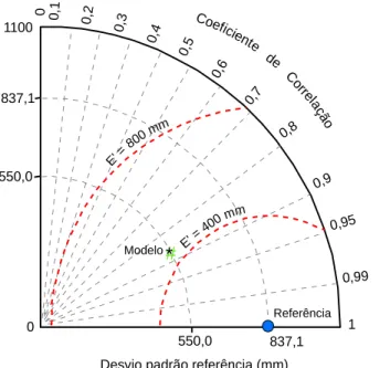
Statistics were represented by the Taylor diagram (Fig. 2) constructed by the representation of a ¼ circle.The x and y axes were used to represent the standard deviation, being that the value of the standard deviation of the observed data is placed on the x axis (r ) and the standard deviation of the values simulated by the models is placed on the y axis (f
). The radial distance from the origin to the position representing the other model is proportional to and the azimuth is given by the correlation (R). f
Fig. 2 Taylor Diagram displaying statistics with a ¼ circle.
Performance evaluation of models for climate variables is of fundamental importance in studies on climate change impacts, since that with the provided data we can try to understand possible changes that are occurring in the global climate and that will occur in the future. The performance of the models is based on the similarity between the simulated data through models and observed data for the area of interest (Taylor, 2001; Tebaldi e Knutti 2007).
In view of the above, this study aims to evaluate the performance of the 22 global climate models from the IPCC- AR4 as well as the Multi-model (ensemble) – MM which is the combined mean of the data from all the different models, in the simulation of climatic data
Coeficien te de C orrela ção 0,1 # * 0 0,2 0,3 0,4 0,5 0,6 0,7 0,8 0,9 0,95 0,99 1 D e s v io p a d rã o d o m o d e lo ( m m ) 550,0 837,1
Desvio padrão referência (mm)
Referência Modelo 837,1 550,0 E'= 400 m m E' = 800 mm 0 1100
Braz. J. of Develop.,Curitiba, v. 6, n.5, p.31241-31260 may. 2020. ISSN 2525-8761 from climatological air temperature variables and pluviometric precipitation for the annual and monthly period in South America
2 METHODOLOGY
2.1 STUDY AREA
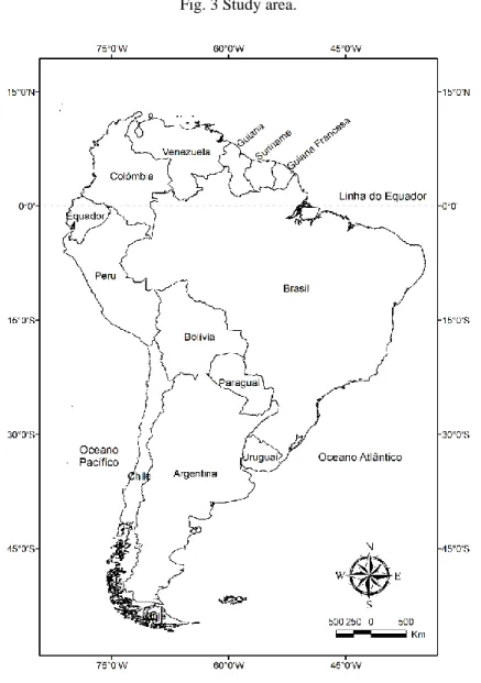
The study area corresponds to the South America continent, with a total area of 17,632,900 km2. It lies geographically between the 83° and 33° west longitude meridians and between the 58° south latitude parallel and 15° north latitude parallel, comprising of Argentina, Bolivia, Brazil, Colombia, Chile, Ecuador, Guyana, French Guiana, Paraguay, Peru, Suriname, Uruguay and Venezuela, as shown in Fig. 3.
Braz. J. of Develop.,Curitiba, v. 6, n.5, p.31241-31260 may. 2020. ISSN 2525-8761 2.2 CLIMATOLOGICAL DATA FOR EVALUATING THE PERFORMANCE OF THE CLIMATE SIMULATION MODELS
The observational climatological database, used as a reference for comparing the simulated data, was provided by the “University of East Anglia”/“Climate Research Unit” (CRU) made available free of charge at the URL; http://www.cru.uea.ac.uk/data, showing the mean monthly precipitation and air temperature for the reference period between 1961-1990, with a resolution of 10'x10' (New et al. 2002).
The climatological variables’ data air temperature and precipitation for the current period (1961-1990) from the IPCC-AR4 come from the results of the simulations of global climate models (Table 1), performed by some research centers taking into account the observed concentrations of greenhouse gases during the 20th century and being represented by the simulation scenario known as Climate of the 20th Century (20c3m).
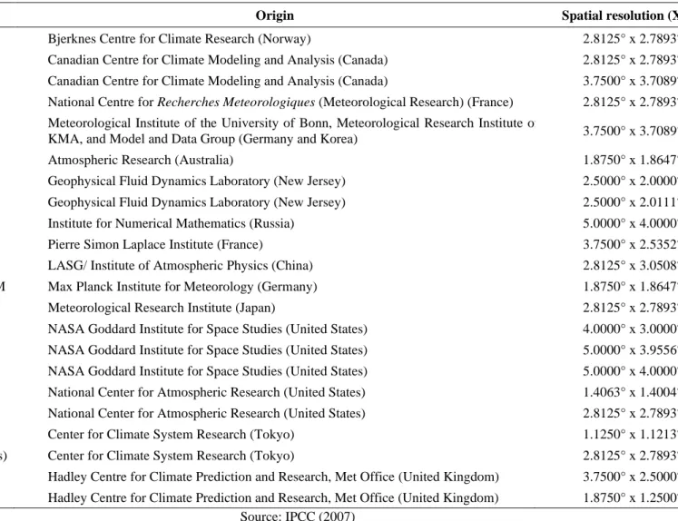
Table 1 Identification, origin and spatial resolution of global climate models from the IPCC-AR4
Model Origin Spatial resolution (X, Y)
BCCR-BCM2.0 Bjerknes Centre for Climate Research (Norway) 2.8125° x 2.7893°
CGCM3.1(T47) Canadian Centre for Climate Modeling and Analysis (Canada) 2.8125° x 2.7893° CGCM3.1(T63) Canadian Centre for Climate Modeling and Analysis (Canada) 3.7500° x 3.7089° CNRM-CM3 National Centre for Recherches Meteorologiques (Meteorological Research) (France) 2.8125° x 2.7893° ECHO-G Meteorological Institute of the University of Bonn, Meteorological Research Institute of
KMA, and Model and Data Group (Germany and Korea) 3.7500° x 3.7089°
CSIRO Mark 3.0 Atmospheric Research (Australia) 1.8750° x 1.8647°
GFDL-CM2.0 Geophysical Fluid Dynamics Laboratory (New Jersey) 2.5000° x 2.0000°
GFDL-CM 2.1 Geophysical Fluid Dynamics Laboratory (New Jersey) 2.5000° x 2.0111°
INM-CM3.0 Institute for Numerical Mathematics (Russia) 5.0000° x 4.0000°
IPSL-CM4 Pierre Simon Laplace Institute (France) 3.7500° x 2.5352°
FGOALS1.0-g LASG/ Institute of Atmospheric Physics (China) 2.8125° x 3.0508°
ECHAM5-MPI-OM Max Planck Institute for Meteorology (Germany) 1.8750° x 1.8647°
MRI-CGCM2.3.2 Meteorological Research Institute (Japan) 2.8125° x 2.7893°
GISS-AOM NASA Goddard Institute for Space Studies (United States) 4.0000° x 3.0000° GISS-EH NASA Goddard Institute for Space Studies (United States) 5.0000° x 3.9556° GISS-ER NASA Goddard Institute for Space Studies (United States) 5.0000° x 4.0000° NCAR-CCSM3 National Center for Atmospheric Research (United States) 1.4063° x 1.4004° NCAR-PCM National Center for Atmospheric Research (United States) 2.8125° x 2.7893°
MIROC3.2 (hires) Center for Climate System Research (Tokyo) 1.1250° x 1.1213°
MIROC3.2 (medres) Center for Climate System Research (Tokyo) 2.8125° x 2.7893°
HADCM3 Hadley Centre for Climate Prediction and Research, Met Office (United Kingdom) 3.7500° x 2.5000° HadGEM1 Hadley Centre for Climate Prediction and Research, Met Office (United Kingdom) 1.8750° x 1.2500°
Braz. J. of Develop.,Curitiba, v. 6, n.5, p.31241-31260 may. 2020. ISSN 2525-8761
2.3 STANDARDIZATION OF RESOLUTIONS AND WEIGHTING OF
CLIMATOLOGICAL AIR TEMPERATURE AND PLUVIOMETRIC PRECIPITATION DATA FROM THE IPCC-AR4
The first step consisted of obtaining a grid with a spatial resolution value that is common for all 22MCGs from the IPCC-AR4, since the models were found to have different resolutions. In order to do this, the calculation for the mean spatial resolution of all models proceeded, performing later interpolation of all cells to the value that comes from the result of the resolution mean from 22 MCGs from the IPCC-AR4 (3.0384° longitude x 2.6685° latitude).
The second step was to adjust the climate data resolution of the CRU to the same grid resolution found for the MCGs (3.0384° x 2.6685°), but as the CRU’s resolution was 10' x 10', it was necessary to consider the mean climatic variable values of the cells that were included in the new resolution, however for the annual period of climatic precipitation variable, the values in the cells were added together. The methodology as described above was adopted in studies performed by Lambert and Boer (2001); Radic and Clarke (2011).
The third step was weighing the values of each cell according to its area, since cells close to the Ecuador have varying values from that of a cell further away
For example, a cell that is on the Equator with the spatial resolution of 3.0384° x 2.6685° will correspond to an area of approximately 95567 km2. On the other hand, a different
cell with this same resolution, on latitude of -50, will have an area of approximately 64000 km2. The weighted mean () of standard deviation for the observed data and the simulated
data of a variable (x ) through the area of each cell ( w ) is given in Eq. 1.
= i i i i i w x w w x; ) ( (1)The weighted (R) correlation through the area of each cell between two variables, x
(observed) and y (simulated) is given as in Eq. 2.
cov(x,x;w)cov(y,y;w) ) w ; y , x ( cov ) w ; y , x ( R = (2) where:
Braz. J. of Develop.,Curitiba, v. 6, n.5, p.31241-31260 may. 2020. ISSN 2525-8761
− − = i i i i i i w w y y w x x w w y x, ; ) ( ( ; ))( ( ; )) cov( (3)In this way the standard deviation will be given as in Eq. 4.
− = i i i i i w )) w ; x ( x ( w ) w ; x ( 2 (4)In addition to the statistics described above, the term “bias” was also adopted (E), which is the difference between the mean simulated ( f ) and observed (r) values of weighted data, as defined by Eq. 5.
E = f −r (5)
The models’ performance evaluation was completed by comparing weighted statistical indexes from the CRU (observed) and simulated data from the IPCC-AR4 models, being that the more similar the simulated were to the observed data, the better the model’s performance.
2.4 TAYLOR DIAGRAM METHOD
The Taylor diagram method can be applied with data from various areas. In this study the method is used with simulated and observed climatic data for the annual and monthly period for climate air temperature and pluviometric precipitation variables. Thus, when using simulated future climatological data by models, the performance and the ability of the model to simulate the data of climatic variables of interest should be noted. It is assumed that the model that presents the best performance on simulating the current climate is also the best for the simulating future climate projections.
Through using the Taylor diagram, it was possible to show four statistical indexes together in a single chart, these indexes were used as a criterion in evaluating the performance of the models. When constructing the Taylor diagram two variables were considered, one with the observed data (
r
) used as a reference and the other with the simulated data ( f ) accordingto a random mathematical model. One of the most commonly used statistics in observing the model’s performance is through comparison through square root of the mean squared of the differences (E) between f and
r
given in Eq. 6:Braz. J. of Develop.,Curitiba, v. 6, n.5, p.31241-31260 may. 2020. ISSN 2525-8761 E (f r) f r f rR 2 2 2 2 2 2 + − + − = (6) where:
f = mean of the simulated data;
r
= mean of the observed data; f
= standard deviation of simulated data;
r
= standard deviation of the observed data; and
R = correlation coefficient.
The square root of the mean squared of the centered differences (E') as described in Eq. 7 is also a widely used statistical index in the evaluation of the IPCC climate performance models. E' f r f rR 2 2 2 2 2 + − = (7)
In Eq. 7 four statistics can be found (E',f,r,R) which were used to study the
relationship pattern between f and
r
in order to show whether the model is a good estimator. These statistics are analyzed together allowing observation of the degree of similarity of the models with reference data.Performance evaluation of the MCGs from the IPCC-AR4 was performed for the annual and monthly period, and for analyzing the annual period for the variable precipitation, the annual amount of precipitation was the sum of the monthly figures, while the climatic air temperature variable was performed using mean annual values. Considering the statistical indexes of each model, it was possible to evaluate their performance by comparing reference data (CRU), so the smaller E' is, the better the model’s performance in simulating climate
data of the studied variable.
Organization of climate data from CRU and IPCC-AR4, calculations of statistical indexes and the generation of Taylor diagrams were performed through the construction of functions in programming language developed in Matlab ® 6.5 software, this was of fundamental importance in the development of the study as it allowed the analysis of a large amount of data.
Braz. J. of Develop.,Curitiba, v. 6, n.5, p.31241-31260 may. 2020. ISSN 2525-8761
3 RESULTS AND DISCUSSION
Using the Taylor diagram, it was possible to jointly see four statistical indexes of fundamental importance in assessing the performance of the models, such as the standard deviation of the observed data and IPCC-AR4 models (r and f ) respectively, square root of the mean squared of the centered differences (E') and the correlation coefficient (R) at the same time, facilitating the analysis of the results.
3.1 PERFORMANCE OF GLOBAL CLIMATE MODELS FOR THE SIMULATION OF THE ANNUAL AND MONTHLY AIR TEMPERATURE MEANS
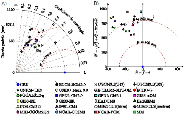
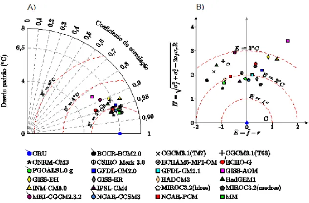
Fig. 4 presents the Taylor diagram with the statistical indexes of mean annual precipitation and individualized model errors through complementary statistical information such as the “bias” (E), which is the difference between the means of the simulated and observed values. Simulated data from 22 global climate models from the IPCC-AR4 as well as the Multi-model (ensemble) – MM were considered, comprised between 1961 and 1990 (20c3m), these were compared with the observed data from the CRU for the same period.
Fig. 4 Taylor diagram displaying the comparison of statistical indexes of observed data (CRU) and climatic simulation models from the IPCC AR4 [A], and the “bias” graph showing the individual errors in climate models [B], considering 1961-1990 (20c3m) for annual precipitation.
Braz. J. of Develop.,Curitiba, v. 6, n.5, p.31241-31260 may. 2020. ISSN 2525-8761 A model is considered to have a high-performance when it presents the simulated standard deviation value closest to the observed, a high correlation and a low value ofE'. Adopting the smallest E'value along with the other statistical indexes in the evaluation of the models’ performance as a criterion, it is observed that the MRI-CGCM 2.3.2 model had the best performance when compared to the others for the annual mean precipitation (Fig. 4A).
Yet, according to Fig. 4A, one can see that the GFDL-CM2.1 and NCAR-PCM models obtained the worst results for E' and R , therefore presenting a low performance. The correlation (R) of simulated data through the 22 models from IPCC and through the Multi-model (ensemble) – MM varied between 0.3 to 0.8, the closer to 1 the better the simulated data are correlated with the observed data.
Through Fig. 4B it is possible to analyze the “bias” (E), note that those models that are represented on the left side of the x-axis from the 0 value underestimated precipitation, while HADCm3 that is depicted on the right side was the only one which overestimated precipitation, peaking at almost 200mm when compared to CRU data. All other models underestimated precipitation values, highlighting the INM model-3.0 CM which was most exaggerated in the amplitude of the simulation with almost 550mm.
Yet in Fig. 4B it is possible to notice that all models presented significant differences among them in the simulation of annual precipitation values, and also when compared to the observed. Marengo (2007) notes that the uncertainties presented by the models in the projections of precipitation are still high.
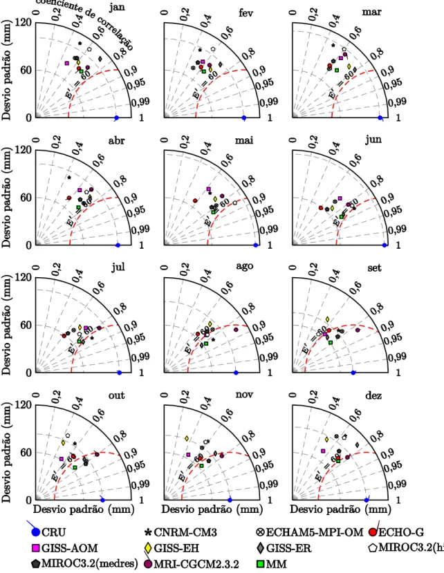
In Fig. 5 the Taylor diagram is presented with the results of statistical indexes of monthly mean values of pluvial precipitation between 1961 -1990 (20c3m), for the best 10 MCGs from IPCC-AR4 and Multi-model (ensemble) – MM, in addition to the data observed by CRU. The models’ behavior results for the months of the year were obtained by means of the monthly mean of all weighted statistical indexes of the variable pluviometric precipitation. The 10 best models were adopted for easy viewing of the same in the diagram.
According to Fig. 5 the Multi-model (ensemble) – MM which presented the best performance when compared to individual models, showing a (R) value of 0.76 and (E') 62.75, this last index being the adopted criteria for choosing the best model.
Gleckler et al. (2008); Reichler and Kim (2008); Pierce et al. (2009) evaluated the simulation of the GCMs from IPCC-AR4 for climate variables and concluded that the performance of the joint multi-model (ensemble) – MM was superior when compared to the
Braz. J. of Develop.,Curitiba, v. 6, n.5, p.31241-31260 may. 2020. ISSN 2525-8761 performance of any individualized model. Pierce et al. (2009) also attributed the results to the error distribution when the mean is calculated between the models.
Combinations of different models can be used in various studies, not being limited only to climate change studies, demonstrating that the multi-model (ensemble) – MM increases the consistency and reliability of simulated data. Among their applications are in the public health sector which used climate projections of multi-model (ensemble) – MM in malaria alerts (Thomson et al. 2006) and in agriculture which used a combination of several models so as to make predictions for crop yields, the results were reported as superior when compared to just a single model (Cantelaube and Terres, 2005).
Brekke et al. (2007) assessed the importance of global climate models from the IPCC-AR4 on climate change estimate projections for analyzing possible hydroclimatologic risks during the dry and rainy seasons, and observed that the multi-model (ensemble) – MM was also what presented better results for data simulation when compared to the data from individualized models.
Studies by Silveira et al. (2011) when evaluating the performance of the MCGs from the IPCC-AR4, regarding the year-to-year pluviometric precipitation variability over Northeastern Brazil, the Amazon and the Platine region located in southern Brazil, pointed to the GISS-ER model as the best in the data simulation for the Amazon region, the CSIRO Mark 3.0 for the Northeastern region of Brazil and the CGCM3.1 (T47) e o CGCM3.1 (T63) models for the Platine region, however, the study does not cover the combination of data from different models of the IPCC (Multi-model (ensemble) – MM). The authors state that these models can be considered as a good option for studies on the effects of climate change on water resources in South America.
Braz. J. of Develop.,Curitiba, v. 6, n.5, p.31241-31260 may. 2020. ISSN 2525-8761 Fig. 5 Taylor diagram displaying the comparison of statistical indexes of the observed data (CRU) and the 10 best global climate models from the IPCC-AR4 from between 1961 -1990 (20c3m) for monthly mean precipitation.
Fig. 5 shows that in the months from January to March, the GISS-ER model presented the best performance when compared to others, even though this same behavior was not
Braz. J. of Develop.,Curitiba, v. 6, n.5, p.31241-31260 may. 2020. ISSN 2525-8761 repeated in other months. It is also noted that the CNRM-CN3 model’s performance was well below the other models in the period from January to April, with improved performance over the other months.
3.2 PERFORMANCE OF GLOBAL CLIMATE MODELS FOR SIMULATIONS OF THE ANNUAL AND MONTHLY AIR TEMPERATURE MEANS
Fig. 6 presents a Taylor diagram with the statistical annual mean indexes of observed and simulated data for the annual mean temperature climate variable and individualized model errors through “bias” (E ). For the analysis of this variable the simulated data by IPCC-AR4 models were also considered in addition to the Multi-model (ensemble) – MM and the data from 1961-1990 (20c3m).
According to Fig. 6A, the observed value of the standard deviation from the CRU data was 6.5, while the ECHO-G model showed the biggest difference between the value of standard deviation from simulated and observed data, which was approximately 1.4.
Analyzing the correlation between simulated and observed data shows that the GISS-AOM model had the worst degree of correlation between all others (0.85), while the majority obtained correlation higher than 0.9 (Fig. 6A).
For annual means of the data, the CNRM-CM3 model presented the best performance when compared to the others with (E' ) of 1.49 and (R) of 0.97 followed by Multi-model (ensemble) – MM which presented similar results (E' ) of 1.65 and (R) of 0.97.
Fig. 6B shows that it is possible to conclude that the models had different behaviors in the simulation of air temperature data, since they are represented far apart from each other. Those which are represented on the left side of the x-axis, from value 0 are underestimating the temperature, while the ones on the right side overestimate. This analysis was only made possible through the “bias” ( E ), which showed that the models could overestimate or underestimate the temperature up to 2°C when compared to the observed data. Among the overestimated values, the GISS-AOM model had the greatest amplitude value; approximately 1.6° C of observed air temperature, and for the underestimated values, the BCCR-BCM2.0 which had a value of approximately 1.5°C was highlighted.
Braz. J. of Develop.,Curitiba, v. 6, n.5, p.31241-31260 may. 2020. ISSN 2525-8761 Fig. 6 Taylor diagram displaying the comparison of statistical indexes from observed data (CRU) and climate simulation models from the IPCC-AR4 (A), and the “bias” graph showing the climate models’ individual errors (B), considering 1961-1990 (20c3m) for the mean annual temperature.
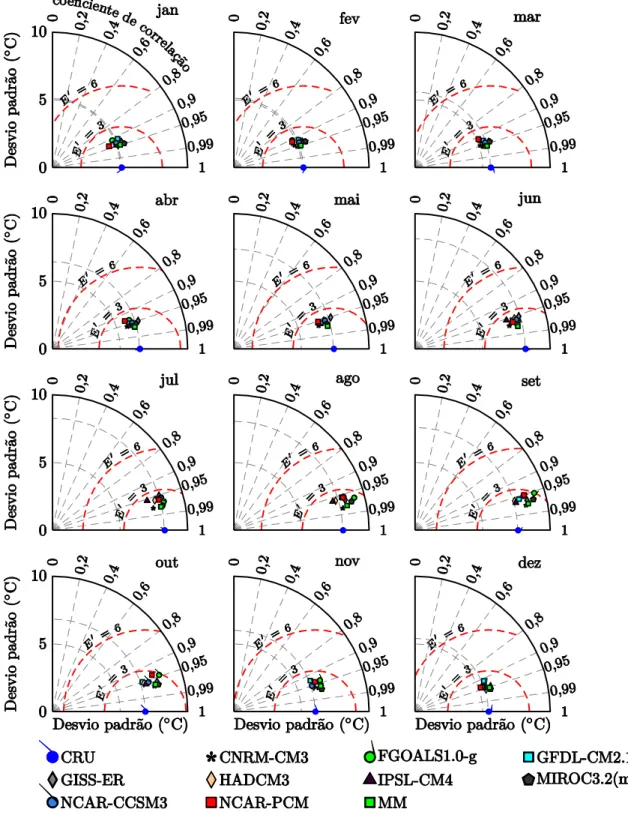
Fig. 7 presents a Taylor diagram with the results of statistical indexes from monthly mean air temperature values between 1961 -1990 (20c3m), for the best 10 MCGs from IPCC-AR4 and Multi-model (ensemble) – MM, in addition to the observed data by CRU. The models’ behaviour results for the months of the year were obtained by means of the monthly mean of all considered statistical indexes.
In Fig. 7, it can be observed that from November to May the models behaved similarly in the simulation of temperature values, the same did not occur for the other months of the year, where there was greater amplitude in the simulation of data, because they are more distant from each other. Air temperature data simulated by the models were well correlated with the observed data, obtaining values greater than 0.9.
Generally speaking, the Multi-model (ensemble) – MM was the model that showed the best performance for temperature data simulation when compared to other models. This result can also be confirmed in the study performed by Pierce et al. (2009), which emphasizes the superiority of the Multi-model (ensemble) – MM when compared to individualized models.
Concurring results were found by Radic & Clarke (2011), who analyzed the performance of the 22 MCGs from IPCC-AR4 and the combination of these in the data
Braz. J. of Develop.,Curitiba, v. 6, n.5, p.31241-31260 may. 2020. ISSN 2525-8761 simulation of various climatic variables, such as precipitation and air temperature for North America. The results demonstrated that the Multi-model (ensemble) – MM was superior to any individual model in the data simulation of the analyzed climatic variables.
Lambert and Boer (2001) performed evaluation and comparison studies of climatic data simulation with 15 IPCC global climate models and concluded that the combination of various Multi-model (ensemble) – MM showed improved results, i.e. much more similar to the observed data mean, when compared with the mean of just a single model. The authors also point out that different climatic variables are simulated with different levels of success for different models and that a single model may not be best for all climatic variables.
Gillett et al. (2002), emphasizes the superiority of Multi-model (ensemble) – MM in relation to the individual models when studying greenhouse gases that contribute to global warming. Palmer et al. (2005) also highlighted the relevance of the Multi-model (ensemble) – MM in climate change studies, reporting that the projections simulated by combining different models show a greater reliability and consistency in data when compared to the data of only one model, this may be justified due to the error distribution when the mean is calculated among the models.
Comparing Fig. 5 and 7, one can see that the models have a much more similar behavior to each other when comparing variable climatic air temperature data than the pluviometric precipitation data. This can be noticed through the position of the models in the Taylor diagram, being that the closer they are to each other, the more similar the simulated results are for them.
Braz. J. of Develop.,Curitiba, v. 6, n.5, p.31241-31260 may. 2020. ISSN 2525-8761 Fig. 7 Taylor diagram displaying the comparison of statistical indexes of the observed data (CRU) and the 10 best global climate models from the IPCC-AR4 considering 1961 -1990 (20c3m) for mean monthly temperature.
4 CONCLUSION
The Taylor diagram method has become an important tool in assessing the performance of the MCGs from the IPCC-AR4, since it allows statistical indexes of interest to be
Braz. J. of Develop.,Curitiba, v. 6, n.5, p.31241-31260 may. 2020. ISSN 2525-8761 simultaneously displayed on a single diagram. The Multi-model (ensemble) – MM was superior in data simulation of the monthly means for pluviometric precipitation and air temperature. Climate projections conducted by combining a set of models is a relatively recent topic in climate research and has gained great momentum in recent years, being greatly used as strategies in decision making processes. When analyzing the annual period, the MRI-CGCM 2.3.2 model presented the best performance for precipitation, while for air temperature the CNRM-CM3 model is highlighted as that which presented the best performance. It is important to note that MCG's from the IPCC-AR4 have a certain degree of uncertainty in climate change projections, since they are not totally accurate, because they still require a few years of study and are constantly evolving. No matter how good the models’ performances are, any projection for the climate is always conditioned to the considered scenario, in view of mankind’s unpredictable behavior. Perfect climate projections are probably impossible to obtain due to uncertainties in emission scenarios, however, MCGs are indispensable tools in future studies on climate change, and the assessment of their performance is of great importance for their applications.
ACKNOWLEDGMENTS
To the Instituto Federal do Espírito Santo (Federal Institute of Espírito Santo) (IFES) for their financial support in this article’s translation.
REFERENCES
Assad ED, Martins SC, Beltrão NEM, Pinto HS. Impacts of climate change on the agricultural zoning of climate risk for cotton cultivation in Brazil. Pesquisa Agropecuária Brasileira, Brasília, v.48, n.1, p. 1-8, jan. 2013.
Buckeridge, M.S.; Aidar, M.P.M.; Silva, E.A.; Martinez,C.A. Respostas de Plantas às Mudanças Climáticas Globais. In: Buckeridge, M.S. (Org.). Biologia e Mudanças Climáticas no Brasil. 1.ed. São Carlos: Rima Editora, v. 1, p.77-91, 2008.
Brekke, L. D.; Dettinger, M. D.; Maurer, E. P.; Anderson, M. Significance of model credibility in estimating climate projection distributions for regional hydroclimatological risk assessments. Climatic Change, n. 89, p. 371–394, 2007.
Cantelaube, P.; Terres, J. M. Seasonal weather forecasts for crop yield modelling in Europe. Tellus Series A-dynamic Meteorology And Oceanography, v.57, p. 476–487, 2005.
Coquard, J.; Duffy, P. B.; Taylor, K. E. Present and future surface climate in the western U.S. as simulated by 15 global climate models. Climate Dynamics, n. 23, p. 455–472, 2004.
Braz. J. of Develop.,Curitiba, v. 6, n.5, p.31241-31260 may. 2020. ISSN 2525-8761 Gillett, N. P., Zwiers, F. W., Weaver, A. J., Hegerl, G. C., Allen, M. R. & Stott, P. A. Detecting anthropogenic influence with a multi-model ensemble. Geophysical Research Letters. v. 29, n. 20, p. 1-4, 2002.
Gleckler, P. J.; Taylor, K. E.; Doutriaux, C. Performance metrics for climate models. Journal of Geophysical Research, v. 113, D06104, p. 1-20, 2008.
Intergovernmental Panel on Climate Change (IPCC) 2007, IPCC fourth assessment report – climate change 2007: the physical science basis. Summary for Policymakers.
Lambert, S. J.; Boer, G. J. CMIP1 evaluation and intercomparison of coupled climate models. Climate Dynamics, v. 17, p.83-106, 2001.
Marengo J. A. Cenários de Mudanças Climáticas para o Brasil em 2100. Ciência & Ambiente, v. 34, p. 100-125, 2007.
Mendicino, G.; Senatore, A. Evaluation of parametric and statistical approaches for the regionalization of flow duration curves in intermittent regimes. Journal of Hydrology, v.480, p.19-32, 2013.
New, M.; Lister, D.; Hulme, M.; Makin, I. A high-resolution data set of surface climate over global land areas. Climate Research, v. 21, p. 1-25, 2002.
Palmer, T.; Shutts, G.; Hagedorn, R.; Doblas-Reyes, F.; Jung, T.; Leutbecher, M. Representing model uncertainty in weather and climate prediction. Annu Review Earth Planetary Science, v. 33, p. 163–193, 2005
Pierce, D. W.; T. P. Barnett.; B. D. Santer.; P. J. Gleckler. Selecting global climate models for regional climate change studies. Proceedings of the National Academy of Sciences, USA, v.106, n. 21, p. 8441–8446, 2009.
Radic, V.; Clarke, G. K. C. Evaluation of IPCC Models’ Performance in Simulating Late-Twentieth-Century Climatologies and Weather Patterns over North America. Journal of Climate, v. 24, p. 5227-5274, 2011.
Reichler, T.; Kim, J. How well do coupled models simulate today’s climate? American Meteorological Society, v. 89, p. 303–311, 2008.
Silveira, C. S.; Souza Filho, F. A.; Lázaro, Y.M. C.; Costa, A. C.; Sales, D. C.; Coutinho, M.M. Avaliação do desempenho dos modelos de mudanças climáticas do IPCC-AR4 quanto a sazonalidade e o padrões de variabilidade interanual da precipitação sobre o nordeste setentrional brasileiro nas simulações do IPCC-AR4. Revista Brasileira de Recursos Hídricos, v.18, n.1, p.177-194, 2013.
Stevens, B.; Giorgetta, M.; Esch, M.; Mauritsen, T. Crueger, T.; Rast, S.; Salzmann, M.; Schmidt, H.; Bader, J.; Block, K.; Brokopf, R.; Fast, I.; Kinne, S.; Kornblueh, L.; Lohmann, U.; Pincus, R.; Reichler, T.; Roeckner, E. Atmospheric component of the MPI-M earth system model: ECHAM6. Journal of Advances in Modeling Earth Systems, v. 5, p. 146-172, 2013. Taylor, K. E. Summarizing multiple aspects of model performance in a single diagram. Jounal of Geophysical Research, v. 106, n. (D7), p. 7183–7192, 2001.
Tebaldi, C.; Knutti, R. The use of the multimodel ensemble in probabilistic climate projections. Philosophical Transactions of the Royal Society A, London, n. 365, p. 2053–2075, 2007.
Thomson, M. C.; Doblas-Reyes, F. J.; Mason, S. J., Hagedorn, R.; Connor, S. J.; Phindela, T.; Morse, A. P.; Palmer, T. N. Malaria early warnings based on seasonal climate forecasts from multi-model ensembles. Nature, v. 439, p.576–579, 2006
Zullo Jr, J.; Pinto, H. S.; Assad, E. D.; Ávila, A. M. H. Potential for growing Arabica coffee in the extreme south of Brazil in a warmer world. Climatic Change, v.109, p. 535