Source points placement in the method of fundamental solutions for parabolic
problems
Colocação de pontos de fonte no método de soluções fundamentais para
problemas parabólicos
DOI:10.34117/bjdv6n3-041
Recebimento dos originais: 30/01/2020 Aceitação para publicação: 04/03/2020
Carlos Eduardo Polatschek Kopperschmidt
Mestre em Engenharia Mecânica pela Universidade Federal do Espírito Santo Instituição: Universidade Federal do Espírito Santo
Endereço: Av. Fernando Ferrari, 514 - Goiabeiras, Vitória - ES, Brasil E-mail: cadupolkop@gmail.com
Bruno Henrique Marques Margotto
Mestre em Engenharia Mecânica pela Universidade Federal do Espírito Santo Instituição: Universidade Federal do Espírito Santo
Endereço: Av. Fernando Ferrari, 514 - Goiabeiras, Vitória - ES, Brasil E-mail: brunohmmargotto@gmail.com
Wellington Betencurte da Silva
Doutor em Engenharia Mecânica pela Universidade Federal do Rio de Janeiro Instituição: Universidade Federal do Espírito Santo
Endereço: Alto Universitário, S/N Guararema, Alegre - ES, Brasil E-mail: wellingtonufes@gmail.com
Júlio César Sampaio Dutra
Doutor em Engenharia Química pela Universidade Federal do Rio de Janeiro Instituição: Universidade Federal do Espírito Santo
Endereço: Alto Universitário, S/N Guararema, Alegre - ES, Brasil E-mail: juliosdutra@yahoo.com.br
ABSTRACT
In this paper, the placement of the source points for Method of Fundamental Solutions in one-dimensional parabolic partial differential equations is evaluated for two different traditional benchmark problems one with Dirichlet condition and other with mixed boundary conditions. Four source points placement strategies are used. The approximate results from Method of Fundamental Solutions are sensitive to strategy used, and when the positive timed source points are used the approximate results are instable.
Keywords: Method of Fundamental Solutions, Time-dependent, Parabolic, Heat conduction
problem.
RESUMO
Neste artigo é investigado o posicionamento dos pontos-fonte no contexto do Método das Soluções Fundamentais para equações diferenciais parciais parabólicas em uma dimensão para dois problemas típicos de benchmark, um com condições de Dirichlet e outro com condições mistas. Quatro estratégias diferentes para o posicionamento dos pontos-fonte são utilizadas. Os resultados
aproximados a partir do Método das Soluções Fundamentais demonstram-se sensíveis à estratégia de posicionamento utilizada, e pontos-fonte com coordenadas positivas para o tempo promovem resultados instáveis.
Palavras-chave: Método das Soluções Fundamentais, Transiente, Parabólico, Problema de
Condução de Calor.
1 INTRODUCTION
The Method of Fundamental Solutions (MFS) is a meshless method proposed by Kupradze & Aleksidze (1964). A numerical implementation of this method was discussed by Mathon & Johnston (1997). Initially used to obtain the solution for elliptic PDEs, the MFS gained popularity in recent years for heat transfer problems.
The application of MFS in dependent problems is commonly associated with time-marching process, Valtchev & Robertty (2008) developed a time-time-marching MFS scheme for heat conduction problems, where the general heat transfer problem is modified into an inhomogeneous Helmholtz problem, that can be solved as an elliptic boundary value problem with a Crank-Nicolson scheme to make a time-update. Lin et al. (2010) extends the time-marching MFS to multi-dimensional telegraph equations modified into a Poisson type equation using the Houbolt scheme obtaining good efficiency and accuracy including irregular domain.
Parabolic boundary problems can be related to the application of time-dependent fundamental solutions on the MFS. This approach is widely discussed in recent work by Johansson (2017) both for direct and inverse problems. In this paper, the MFS with time-dependent fundamental solutions approach is discussed in relation to placement of the source points and its influence on the accuracy of approximated solutions.
2 MATHEMATICAL FORMULATION
2.1 CASE 1
In Case 1, a typical backward heat conduction problem (BHCP) benchmark example previously discussed in Mera (2006) and Grabski (2019) is investigated. We consider a solution domain Ω ⊂ 𝑅𝑑, 𝑑 = 1, and we assume that the temperature on the boundary of the domain as well as the temperature distribution inside the solution domain at time 𝑡∗ is known. Thus, governing
equation is given by the parabolic equation Eq. (1), that satisfies conditions of Eq. (2) and Eq. (3). The analytical solution is given by Eq. (4).
𝜕𝑢
𝜕𝑡 (𝑥, 𝑡) = ∇
2𝑢(𝑥, 𝑡) (𝑥, 𝑡) ∈ Ω × (0, 𝑡
𝑢(𝑥, 𝑡) = 𝑓(𝑡) 𝑥 ∈ 𝜕Ω (2)
𝑢(𝑥, 𝑡∗) = 𝑔(𝑥) 𝑥 ∈ Ω (3)
𝑢(𝑥, 𝑡) = sin(𝜋𝑥) 𝑒−𝜋2𝑡, (𝑥, 𝑡) ∈ [0,1] × [0, 𝑡𝑓] (4)
For Case 1, when 𝑡 = 0, 𝑔(𝑥) = sin(𝜋𝑥), the exponential term is suppressed on the boundary and initial conditions. Otherwise, if 𝑡∗ increase, 𝑔(𝑥) decrease and tends to zero and the information
are very weak. Then, the boundary conditions are Dirichlet conditions like in Eq. (5), and 𝑔 is given by Eq (6), in terms of 𝑡𝑓= 1.
𝑓(𝑡) = 0, 𝑥 = 0 , 𝑥 = 1 , 𝑡 ∈ [0, 𝑡𝑓] (5)
𝑔(𝑥) = sin(𝜋𝑥) 𝑒−𝜋2𝑡𝑓, 𝑥 ∈ (0,1) , 𝑡
𝑓 = 1 (6)
2.2 Case 2
In Case 2, a typical benchmark Robin condition problem previously presented by Yan et al. (2009) is discussed. Assuming the same assumptions of Case 1, but considering a Robin data on boundary, the governing equation (Eq. (7)) satisfies the boundary conditions in Eq. (8) and Eq. (9), and the initial conditions in Eq. (10).
𝜕𝑢 𝜕𝑡 (𝑥, 𝑡) = ∇ 2𝑢(𝑥, 𝑡) , (𝑥, 𝑡) ∈ Ω × (0, 𝑡 𝑓) (7) − 𝜕𝑢 𝜕𝑥(0, 𝑡) + 𝜌(𝑡)𝑢(0, 𝑡) = ℎ0(𝑡), 𝑡 ∈ [0, 𝑡𝑓] (8) 𝜕𝑢 𝜕𝑥(1, 𝑡) + 𝜌(𝑡)𝑢(1, 𝑡) = ℎ1(𝑡), 𝑡 ∈ [0, 𝑡𝑓] (9) 𝑢(𝑥, 𝑡∗) = 𝑔(𝑥) , 𝑥 ∈ Ω (10)
Where 𝜌(𝑡) is the time-dependent heat transfer coefficient representing the corrosion damage. For simplicity, we use 𝑡𝑓 = 1. The analytic solution of the problem is given by Eq. (11). The data for ℎ0, ℎ1, 𝑔 and 𝜌 are given by Eq. (12), Eq. (13), Eq. (14) and Eq. (15) respectively.
𝑢(𝑥, 𝑡) = 𝑥2+ 2𝑡 + 1, (𝑥, 𝑡) ∈ [0,1] × [0, 𝑡𝑓] (11)
ℎ0(𝑡) = 𝜌(𝑡)(2𝑡 + 1), 𝑥 = 0 , 𝑡 ∈ [0, 𝑡𝑓] (12)
ℎ1(𝑡) = 2 + 𝜌(𝑡)(2 + 2𝑡), 𝑥 = 1 , 𝑡 ∈ [0, 𝑡𝑓] (13)
𝑔(𝑥) = 𝑥2+ 1, 𝑥 ∈ (0,1) , 𝑡 = 0 (14)
𝜌(𝑡) = 𝑡, 𝑡 ∈ [0, 𝑡𝑓] (15)
3 THE METHOD OF FUNDAMENTAL SOLUTIONS
In the Method of Fundamental Solutions, the approximate solution of the PDE is given by the linear combinations of fundamental solutions of the governing equation of the considered problem, given by the Eq. (16).
û(𝑥, 𝑡) = ∑ 𝛼𝑗𝐺(𝑥, 𝑡; 𝑦𝑗, 𝜏𝑗)
𝐽
𝑗=1
(16)
Where (𝑦𝑗, 𝜏𝑗) are the j’th spatial and time coordinate of source points, respectively, 𝐽 is the number of source points used, and 𝛼 are unknow coefficients to be determined. The source points are placed in a pseudo-region, that contains the study region Ω. For one-dimensional transient heat conduction problems, the fundamental solution 𝐺 is given by Eq. (17).
𝐺(𝑥, 𝑡; 𝑦𝑗, 𝜏𝑗) = 𝐻(𝑡 − 𝜏𝑗) √4𝜋 (𝑡 − 𝜏𝑗) 𝑒 −|𝑥−𝑦𝑗| 2 4𝜋 (𝑡−𝜏𝑗) (17)
The 𝐻 is the Heaviside function. For approximative derivative solution, the fundamental solution can be derived. The fundamental solution satisfies exactly the PDE, and for Parabolic problems, additional data related to time and space should be known to satisfy the initial and boundary conditions. This data on this paper is given for collocation in the boundary and domain according to boundary and initial conditions, respectively. The approximate solution for boundary and initial conditions are given by Eq. (18) and Eq. (19).
𝑓(𝑡) = ∑ ∑ 𝛼𝑗𝐺(𝑥∗, 𝑡𝑚; 𝑦𝑗, 𝜏𝑗) 𝐽 𝑗=1 𝑀 𝑚=0 (18) 𝑔(𝑥) = ∑ ∑ 𝛼𝑗𝐺(𝑥𝑛, 𝑡∗; 𝑦 𝑗, 𝜏𝑗) 𝐽 𝑗=1 𝑁 𝑛=1 (19)
Where 𝑥∗ and 𝑡∗indicate a space and time coordinates known. The resulting system of
equations described in Eq. (20) contains 2(𝑀 + 1) collocation points in the boundary, and 𝑁 = 2(𝑀 − 1) in domain. To obtain a square matrix, the number of source points 𝐽 = 4𝑀.
𝐴𝛼 = 𝐵 (20)
Where 𝐴 is the matrix with the fundamental solutions, 𝛼 is an array with unknow coefficients to be determined and 𝐵 is an boundary/initial data array.
3.1 POSSIBLE SOURCE POINTS DISTRIBUTIONS
In this paper, the placement of the source points is based in a recent work (Grabski, 2019), where four different sources distribution are considered for one-dimensional case.
The first placement strategy (a) is given by Eq. (21). This strategy is common in study of MFS for parabolic problems, being found in Chantasiriwan et al. (2009) and Johansson & Lesnic (2009). The second placement strategy (b) is given by Eq. (22). The (b) idea consists in exclude the timed-positive coordinates from (a) to avoid problems with singularities.
𝒂. (𝑦𝑗, 𝜏𝑗) = { 𝑦𝑗 = −𝑑1, 𝜏𝑗 = −1 + (2𝑗 − 1)2 𝐽, 𝑗 = 1,2 … 𝐽 2 𝑦𝑗 = 1 + 𝑑1, 𝜏𝑗 = −1 + (2 (𝑗 − 𝐽 2) − 1) , 𝑗 = 𝐽 2+ 1, 𝐽 2+ 2, … 𝐽 (21)
𝒃. (𝑦𝑗, 𝜏𝑗) = { 𝑦𝑗= −𝑑1, 𝜏𝑗 = −𝑑2 + (2𝑗 − 1)𝑑2 𝐽 , 𝑗 = 1,2 … 𝐽 2 𝑦𝑗= 1 + 𝑑1, 𝜏𝑗 = −𝑑2 + (2 (𝑗 − 𝐽 2) − 1) 𝑑2 𝐽 , 𝑗 = 𝐽 2+ 1, 𝐽 2+ 2, … 𝐽 (22)
The third placement strategy (c) keeps a constant distance in time axis, given by Eq. (23). The fourth placement strategy (d) is an improvement of the third, and it’s given by Eq. (24).
𝒄. (𝑦𝑗, 𝜏𝑗) = { 𝑦𝑗 = (2𝑗 − 1) 1
2𝐽 , 𝜏𝑗 = −𝑑3 } 𝑗 = 1,2, … , 𝐽 (23)
𝒅. (𝑦𝑗, 𝜏𝑗) = { 𝑦𝑗 = −𝑑4 +
(2𝑗 − 1)(1 + 2𝑑4)
2𝐽 , 𝜏𝑗 = −𝑑3 } 𝑗 = 1,2, … , 𝐽 (24)
The scheme for each placement strategy and distances are indicated on Fig. 1.
4 NUMERICAL RESULTS
The numerical experiments use a fixed number of colocation and source points: 𝑀 = 20 and 𝑁 = 38, therefore 𝐽 = 80. For strategies with two 𝑑 parameters, (b) and (d), a 𝑑1 is chosen from bad results from (a) strategy, and 𝑑3 from (c).
In order to investigate the accuracy and the robustness of the method for different source points placement strategy, the maximum error (ME), the root mean square error (RMSE) and the 𝐴 matrix condition number (CN) are determined like in Eq. (25), Eq. (26) and Eq. (27), respectively.
All domain points used on MFS implementation are used to calculate the errors: 2𝑀 points distributed on spatial domain in each (𝑀 + 1) points from 𝑡, including 𝑡𝑖𝑛𝑖𝑡𝑖𝑎𝑙 and 𝑡𝑓𝑖𝑛𝑎𝑙, having a
total of 2𝑀(𝑀 + 1) points. 𝑀𝐸 = max (√(𝑢𝑒𝑥𝑎 − û)2 ) (25) 𝑅𝑀𝑆𝐸 = √∑ (𝑢𝑒𝑥𝑎𝑖− û𝑖) 𝑁𝑃 𝑖=1 2 𝑁𝑃 (26) 𝐶𝑁 = ‖𝐴‖2 ‖𝐴−1‖ 2 (27)
The algorithm implementation of the MFS for transient heat conduction problem was done in MATLAB® on a Core I5, 8gb RAM Laptop. The resulting system of MFS is solved with the singular value decomposition (SVD). The results for the Case 1, for each source points placement strategy are indicated on Fig. 2, Fig. 3, Fig. 4, Fig. 5, Fig. 6, Fig. 7, Fig. 8 and Fig. 9. The number of 𝑑’s (𝑁𝐷) used in each analysis is much bigger than 𝑑𝑓𝑖𝑛𝑎𝑙. For 𝑑𝑓𝑖𝑛𝑎𝑙 = 10 we have 𝑁𝐷 =1000, resulting in ∆𝑑 = 0.01.
The 𝑅𝑀𝑆𝐸 had similar results to 𝑀𝐸 in relation to the tendency of the results, as can be verified on Fig. 2, thereby, the other RMSE results are suppressed in this work.
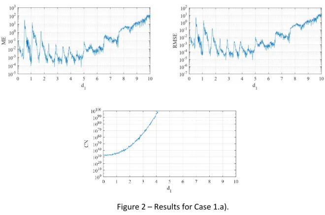
Figure 2 – Results for Case 1.a).
Figure 2 show that with the (a) strategy, the 𝐶𝑁 increases rapidly with increasing 𝑑1, and if 𝑑1 > 5, 𝑀𝐸 and 𝑅𝑀𝑆𝐸 starts to increase indefinitely. The minimum 𝑀𝐸 to Case 1.a) is 𝑶−5, but a
small variation in 𝑑1 can turn the error in 𝑶−2 between 2 < 𝑑1 < 5. Same can be verified in Fig. 6 for Case 2.a).
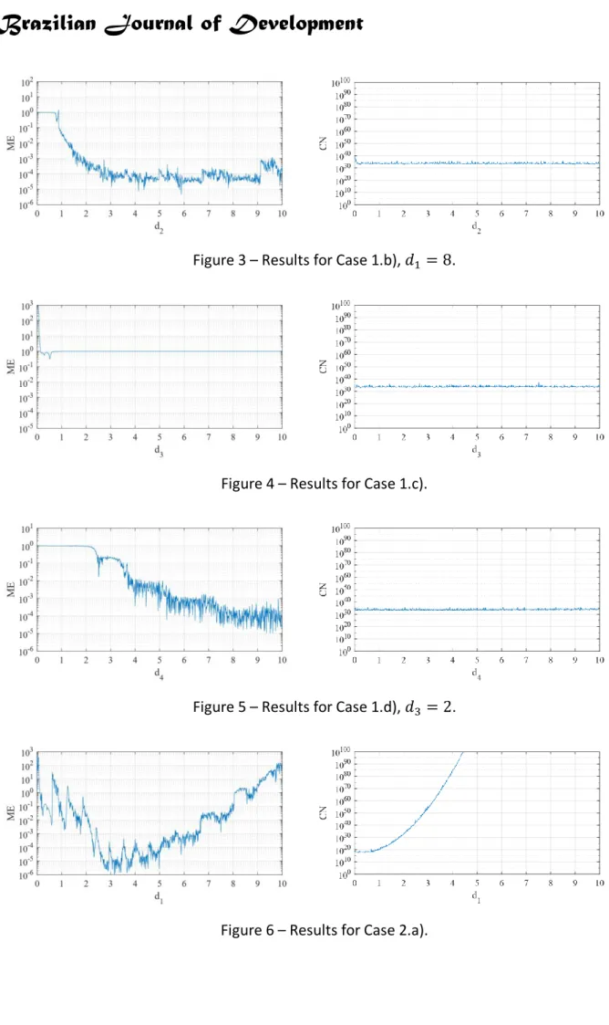
The (b, c and d) strategies, unlike (a), had a smooth behavior from 𝐶𝑁 in all 𝑑 values evaluated on this paper for both Case 1 and Case 2.
In Case 1, (b) and (d) strategies has good results from certain 𝑑2 and 𝑑4 values, Fig. 3 and Fig. 5, respectively. In Case 2.b), Fig. 7, the errors decay rapidly with 𝑑2 and in 𝑑2 > 3 starts to increase, but don’t high than 𝑶−10, while in Case 2.d) (Fig. 9) the errors decays with 𝑑
4 in all values
used.
In Case 1 the strategy (c) don’t presented good results, the errors rapidly stopped in 100, as in
Fig 4. In Case 2, this strategy has the worst minimum error results compared with other and can be viewed in Fig 8. The Fig. 5 show a tendency that if 𝑑4 increases, the error decreases in Case 1, same thing can be verified in Fig. 9 to Case 2.
Figure 3 – Results for Case 1.b), 𝑑1 = 8.
Figure 4 – Results for Case 1.c).
Figure 5 – Results for Case 1.d), 𝑑3 = 2.
Figure 7 – Results for Case 2.b), 𝑑1 = 8.
Figure 8 – Results for Case 2.c).
Figure 9 – Results for Case 2.d), 𝑑3 = 0.5.
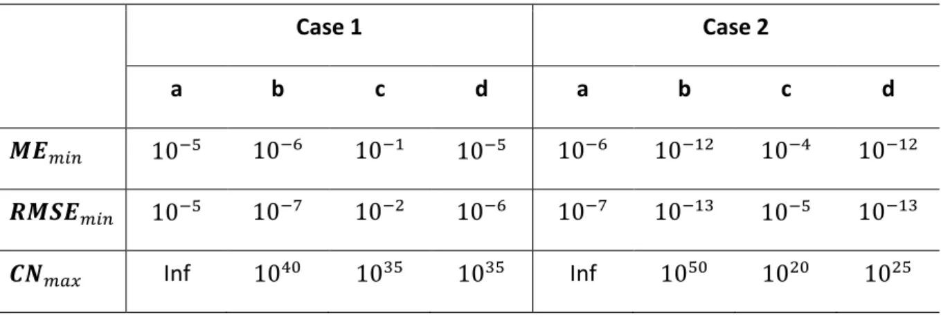
Table 1 – Resumed Results for each strategy Case 1 Case 2 a b c d a b c d 𝑴𝑬𝑚𝑖𝑛 10−5 10−6 10−1 10−5 10−6 10−12 10−4 10−12 𝑹𝑴𝑺𝑬𝑚𝑖𝑛 10−5 10−7 10−2 10−6 10−7 10−13 10−5 10−13 𝑪𝑵𝑚𝑎𝑥 Inf 1040 1035 1035 Inf 1050 1020 1025 5 CONCLUSIONS
The source points distribution is not so trivial. The general conclusion is that the positive-time source points location promotes instabilities in the system of equations from MFS. This could be seen in the (a) strategy results. Although (a) has good results in the literature, the fact that source-points with positive-timed coordinates can spoil the results from temperature field plus the instabilities of this strategy prevents MFS feature from obtaining the solution at each point on domain, not being sufficiently robust for practical problems.
The (b) source points location could determine a high accuracy approximate solution in relation to (a) and (c), and similar accuracy to (d), having better results on Case 1. The (c) strategy shown low accuracy results in both cases, being the worst strategy for source points placement with only negative time placement. In Case 1, this strategy was not effective, having the same results even varying the distance, and in Case 2 presented the worst minimum valor to each evaluated error.
In general sense, (d) was the best possibility to source points placement in relation to its robustness, haven’t presented oscillation and decreasing linearly with 𝑑4, being the easiest strategy to obtain high accuracy.
It is necessary investigate the influence of source points position in other heat conduction problems, especially the (b) and (d) strategies, that were successful in both cases.
The MFS implementation is easy and the approximate results to one-dimensional problems can be very precisely, but the choice of the wrong source points location will spoil the approximation.
ACKNOWLEDGEMENTS
This present work was carried out with the support of the Coordenação de Aperfeiçoamento de Pessoal de Nível Superior - Brazil (CAPES) – Código de financiamento 001 and with support of Edital FAPES/CAPES n° 01/2018.
REFERENCES
Chantasiriwan, S., Johansson, B. T., & Lesnic, D. (2009). “The Method of Fundamental Solutions for free surface Stefan problems”. Engineering Analysis with Boundary Elements, 33(4), 529–538. Grabski, J. K. (2019). “On the sources placement in the Method Of Fundamental Solutions for time-dependent heat conduction problems”. Computers and Mathematics with Applications, https://doi.org/10.1016/j.camwa. 2019.04.023.
Lin, C. Y., Gu, M.H., Young, D. L. (2010), “The Time-Marching Method of Fundamental Solutions for Multi-Dimensional Telegraph Equations”. Tech Science Press. CMC, vol. 18, no. 1, pp. 43-68. Mathon, R., Johnston, R. L. (1977). “The approximate solution of elliptic boundary-value problems by fundamental solutions”. SIAM J. Numer. Anal. 14, 638-650.
Mera, N. S. (2005). The Method of Fundamental Solutions for the backward heat conduction problem. Inverse Problems in Science and Engineering, 13(1), 65–78.
Johansson, B. T., & Lesnic, D. (2009). “A Method of Fundamental Solutions for transient heat conduction in layered materials”. Engineering Analysis with Boundary Elements, 33(12), 1362– 1367. doi:10.1016/j.enganabound.2009.04.014.
Johansson, B. T. (2017). “Properties of a Method of Fundamental Solutions for the parabolic heat equation”. Applied Mathematics Letters, 65, 83–89.doi:10.1016/j.aml.2016.08.021
Kupradze, V. D., & Aleksidze, M. A. (1964). “The method of functional equations for the approximate solution of certain boundary value problems”. USSR Computational Mathematics and Mathematical Physics, 4(4), 82–126.doi:10.1016/0041-5553(64)90006-0
Valtchev, S. S., & Roberty, N. C. (2008). “A time-marching MFS scheme for heat conduction problems”. Engineering Analysis with Boundary Elements, 32(6), 480–493.
Yan, L., Yang, F., & Fu, C. (2009). “A Bayesian inference approach to identify a Robin coefficient in one-dimensional parabolic problems”. Journal of Computational and Applied Mathematics, 231(2), 840–850. Lanzhou University, China.