NEGOTIATING PREFERENTIAL TRADE
AGREEMENTS FOR BRAZIL:
A CGE MODELING PERSPECTIVE
Vera Thorstensen
Lucas Pedreira do Couto Ferraz
(Coordinators)
Rodolfo Arruda Cabral
Carolina Lemos Rêgo
NEGOTIATING PREFERENTIAL TRADE
AGREEMENTS FOR BRAZIL: A CGE
MODELING PERSPECTIVE
VERA HELENA THORSTENSEN
LUCAS PEDREIRA DO COUTO FERRAZ
(Coordenadores)
Carolina Lemos Rêgo
Rodolfo Arruda Cabral
(Autores)
VT
São Paulo
T522 Thorstensen, Vera Helena. Ferraz; Lucas Pedreira do Couto (coordenadores).
Cabral, Rodolfo Arruda; Rêgo, Carolina Lemos (autores).
Negotiating Preferential Trade Agreements for Brazil: A CGE Modeling
Perspective. / Vera Helena Thorstensen; Lucas Pedreira do Couto Ferraz
(coordenadores); Rodolfo Arruda Cabral; Carolina Lemos Rêgo (autores). / São
Paulo: VT Assessoria Consultoria e Treinamento Ltda., 2016.
401p.
Bibliografia
ISBN: 978-85-66977-02-8
1. Economia. 2. Acordos Preferenciais de Comércio. I. Título
CDD 330
Capa, Edição e Diagramação:
Thiago Rodrigues São Marcos Nogueira
© desta edição [2016]
VT Assessoria Consultoria e Treinamento Ltda.
Tel.: (11) 3799-7926
http://ccgi.fgv.br
[email protected]
COORDINATORS
Vera Thorstensen
Professor at São Paulo School of Economics of Fundação Getúlio Vargas (EESP-FGV),
Head of the Center for Global Trade and Investments Studies (CGTI), and Holder of the
WTO Chair in Brazil since 2014. President of the Brazil’s Governmental Committee on
Coordination of Technical Barriers to Trade (CBTC) of INMETRO since 2014. She served
as economic advisor for the Brazilian Mission to the WTO from 1995 to 2010 and
editor-in-chief of Carta de Genebra, published by the Brazilian Mission to the WTO from 2001
to 2008. She also served as Chairperson of the WTO Committee on Rules Origin from 2004
to 2010.
Lucas Pedreira do Couto Ferraz
Lucas Ferraz is Professor of Economics at the São Paulo School of Economics (EESP) from
Fundação Getulio Vargas (FGV). He holds a BD and Masters in Engineering from the
Polytechnic School (POLI) at São Paulo University (USP). He received his PhD in
Economics from Getúlio Vargas Foundation’s Graduate School of Economics
(FGV/EPGE). He participated at the EU scholarship program ALPHA and was a visiting
scholar at the University of Amsterdam, University of Antwerp e University of Brussels.
AUTHORS
Rodolfo Arruda Cabral
Rodolfo Arruda Cabral is a PhD candidate in International Economics at São Paulo School
of Economics (EESP-FGV). He holds a Master in Economics at EESP-FGV, BA in
Economics at Sao Paulo University (USP) and BA in International Relations at Pontifical
Catholic University of Sao Paulo (PUC-SP).
Carolina Lemos Rêgo
Carolina Lemos Rêgo holds a BA in Economics at São Paulo School of Economics
(EESP-FGV) (2016) with a year of studies at the University College London (2015) and the
University St. Gallen (2015). She is a member of the WTO Chair Brazil and a junior
researcher at the Center for Global Trade and Investments (CGTI) of EESP-FGV.
CONTENT
INTRODUCTION ... 7
1.
EXPLAINING THE METHODOLOGY ... 9
1.1.
MODELING
ISSUES ... 9
1.2.
DATA
BASE ... 9
1.3.
RESULTS
OF
THE
SIMULATIONS ... 10
1.4.
REFERENCES ... 10
2.
BRAZIL ... 11
2.1.
SIMULATIONS
OVERVIEW ... 12
2.1.1. Simulation 1 – Brazil x EU – US – China ... 12
2.1.2. Simulation 2 – Brazil x Japan – South Korea – Mexico ... 13
2.1.3. Simulation 3 – Brazil x EU – US – China ... 15
2.1.4. Simulation 4 – Brazil x Japan – South Korea – Mexico ... 16
2.1.5. Simulation 5 – Brazil x EU – US – China ... 18
2.1.6. Simulation 6 – Brazil x Japan – South Korea – Mexico ... 20
2.2.
SIMULATIONS ... 22
2.2.1. Simulation 1 – Brazil x EU – US – China ... 22
2.2.2. Simulation 2 – Brazil x Japan – South Korea – Mexico ... 38
2.2.3. Simulation 3 – Brazil x EU – US – China ... 54
2.2.4. Simulation 4 – Brazil x Japan – South Korea – Mexico ... 70
2.2.5. Simulation 5 – Brazil x EU – US – China ... 86
2.2.6. Simulation 6 – Brazil x Japan – South Korea - Mexico ... 102
3.
MERCOSUL ... 118
3.1.
SIMULATIONS
OVERVIEW ... 119
3.1.1. Simulation 1 – Mercosul x European Union ... 119
3.1.2. Simulation 2 – Mercosul x United States... 120
3.1.3. Simulation 3 – Mercosul x China ... 122
3.1.4. Simulation 4 – Mercosul x European Union ... 124
3.1.5. Simulation 5 – Mercosul x United States... 125
3.1.6. Simulation 6 – Mercosul x Eropean Union ... 127
3.1.7. Simulation 7 – Mercosul x United States... 129
3.1.8. Simulation 8 – Mercosul x China ... 130
3.2.
SIMULATIONS ... 133
3.2.1. Simulation 1 – Mercosul x European Union ... 133
3.2.2. Simulation 2 – Mercosul x United States... 149
3.2.3. Simulation 3 – Mercosul x China ... 165
3.2.4. Simulation 4 – Mercosul x European Union ... 181
3.2.5. Simulation 5 – Mercosul x United States... 197
3.2.6. Simulation 6 – Mercosul x European Union ... 213
3.2.7. Simulation 7 – Mercosul x United States... 229
3.2.8. Simulation 8 – Mercosul x China ... 245
4.
TPP & TTIP ... 261
4.1.
SIMULATIONS
OVERVIEW ... 262
4.1.3. Simulation 3 – Mercosul x TPP – TTIP – TPP + TTIP ... 266
4.2.
SIMULATIONS ... 269
4.2.1. Simulation 1 – Brazil x TPP – TTIP – TPP + TTIP ... 269
4.2.2. Simulation 2 – Argentina x TPP – TTIP – TPP + TTIP ... 300
4.2.3. Simulation 3 – Mercosul x TPP – TTIP – TPP + TTIP ... 331
5.
BRICS ... 362
5.1.
SIMULATIONS
OVERVIEW ... 363
5.1.1. Simulation 1 – BRICS ... 363
5.1.2. Simulation 2 – BRICS ... 364
5.2.
SIMULATIONS ... 366
5.2.1. Simulation 1 – BRICS ... 366
5.2.2. Simulation 2 – BRICS ... 382
ANNEX ... 398
INTRODUCTION
The main objective of this e-book is to present a synthesis of several studies that the Center
for Global Trade and Investment at Fundação Getulio Vargas (CGTI – FGV) has been
producing since 2013. Produced, at first, in an unrelated manner, the works presented in this
Compendium have been revisited and updated so that all simulations became part of a single
body and, therefore, comparable among each other. What is presented in the following pages
is economic information concerning the possible impacts of preferential trade agreements in
the most diverse spheres, aiming to become references to decisions on trade policies,
especially to Brazil.
The scenario for international trade has been under profound transformations. The impasses
on the Doha Round negotiations in the WTO are being solved through small steps in the
Ministerial Conferences of Bali and Nairobi and the proliferation of preferential trade
agreements (PTAs). This scenario has resulted in a transition for the focus of international
trade activities from the multilateral sphere (WTO) to the preferential sphere (PTA).
Preferential agreements, thus, have become the center for rule negotiation and instruments to
trade, expanding the regulatory frontier, with the creation of a series of rules that surpass
WTO’s charter and deepen several themes related to trade, such as services, intellectual
property, investment, environment and competition.
Preferential trade agreements have ceased to simply offer preferential access to goods and
services markets, by means of reduction or elimination of tariffs, establishing instead new
negotiating forums for the currently most important barriers to trade, non-tariff barriers
(NTBs), which comprehend custom barriers, technical barriers, sanitary and phytosanitary
measures, as well as bureaucratic obstacles to trade and, most importantly, costs risen from
regulatory divergences.
With the progressive reduction of tariff barriers through the negotiations of several rounds in
the GATT and WTO, non-tariff barriers have become relevant as the main new obstacle to
international trade, becoming an essential part to the agenda of preferential agreements. Due
to the importance of the theme and the impacts produced by such barriers in the access of
external markets, there no longer exists a single logic in promoting only the negotiation of
preferential tariffs and not also negotiating non-tariff barriers. In such a case, any potential
benefits can be limited significantly without the negotiation of NTBs. These new barriers
were considered throughout the simulations of this e-book.
Any new PTA proposed as an ambitious instrument of trade integration must address not only
the substantial elimination of tariffs, but also trade related issues as customs barriers, technical
barriers, sanitary and phytosanitary measures – including the difficult questions of standard
harmonization and mutual recognition, trade facilitation, services, investment, competition,
intellectual property, regulatory coherence, amongst other topics, which turn negotiations with
new challenges.
Considering such a scenario, Brazil’s position is questionable. The country holds only a
limited number of agreements in force, agreements which also exhibit low ambition in rule
negotiations. The integration of Brazil in international trade has necessarily to go through the
negotiation of new deals, more ambitious ones, with partners of larger importance for Brazil’s
agreements: the Transatlantic Trade and Investment Partnership (TTIP) and the Trans-Pacific
Partnership (TPP). Such agreements cover a significant share of global trade and represent
true paradigms in terms of rules negotiations, which turns the current moment into an
inflexion point concerning Brazil’s international trade policies. The country will certainly
have to rethink its entire agenda if deciding to become once again relevant to the international
scenario. Options for negotiating PTAs with the European Union or with the US, bilaterally or
within TPP or TTIP are discussed in the following chapters, as well as a closer approximation
to BRICS countries.
In synthesis, it is demonstrated that Brazil should quickly leave its isolated status in the sphere
of international trade, confining itself, in past years, in keeping intact Southern Common
Market (Mercosul) and in giving priority to South America. Further to its bonds with
Mercosul, Brazil must have clear perspectives of gains and losses in each of the negotiations
in which it could possibly engage in.
It is precisely on such perspectives that the present e-book aims to shed light.
Vera Thorstensen
1.
EXPLAINING THE METHODOLOGY
1.1.MODELING ISSUES
The GTAP computable general equilibrium model was used in the following simulations in
order to evaluate the first round effects of alternative preferential trade agreements involving
Brazil, amongst other countries. For a description of the standard GTAP model, see Hertel
(1997).
The GTAP model is a global comparative static applied general equilibrium model. The
model identifies 57 sectors in 153 regions of the world. Its system of equations is based on
microeconomic foundations providing a detailed specification of household and perfect
competitive firm behavior within individual regions and trade linkages between regions. In
addition to trade flows, the GTAP model also recognizes global transportation costs.
The GTAP model qualifies as a Johansen-type model. This model estimates the impacts of
external shocks (gains and losses of a PTA) through a comparative static modeling (before
and after the shock). The solutions are obtained by solving the system of linearized equations
of the model. A typical result shows the percentage change in the set of endogenous variables
(GDP, exports and imports, exchange rate and land value) after a policy shock is carried out,
compared to their values in the initial equilibrium, in a given environment. The schematic
presentation of Johansen solutions for such models is standard in the literature (see Dixon et
al (1992) and Dixon and Parmenter (1996)).
For the modeling of the reduction of non-tariff barriers, this project used the same
methodology presented in Ecorys, 2009.
1.2. DATA BASE
The GTAP 9 database combines detailed bilateral trade, transport and protection data
characterizing economic linkages among 140 regions, together with individual country
input-output data bases which account for inter-sectorial linkages within regions. The dataset is
harmonized and completed with additional sources to provide the most accurate description of
the world economy in 2011 (the last available data base for GTAP).
The main applied protection data used in the GTAP 9 data base originates from ITC’s
MacMap database, which contains exhaustive information at the tariff line level. The ITC
database includes the United Nations Conference on Trade and Development’s (UNCTAD’s)
Trade Analysis and Information System (TRAINS) data base, to which ITC staff added their
own data. The model transforms all specific tariffs in ad valorem tariffs.
In order to capture the first round effects from each preferential trade agreement, the
simulations were carried out using a standard GTAP hypothesis, which considers perfect
factor mobility for labor and capital and imperfect factor mobility for land and natural
resources. National aggregate supply of factors of production is exogenous and production
technology for firms is given.
The way the Brazilian economy variables are affected by horizontal reductions in bilateral
import tariffs will depend on the resulting behavior of domestic relative prices. However, in
import competition from the PTA partner will be favored, as the economy becomes more
preferentially open to trade. Overall efficiency in resource allocation tends to be improved
and, by the same token, possible gains from trade may take national welfare a step up.
Notwithstanding the aggregate benefits from improved resource allocation, regions might be
adversely affected through re-orientation of trade flows – trade diversion – as relative
accessibility changes in the system. Thus, bilateral aggregate gains from trade are not
necessarily accompanied by generalized regional gains in welfare. This issue of trade
diversion versus trade creation has been an important one in the international trade literature,
especially in the case of welfare evaluations of preferential trade agreements.
1.3.RESULTS OF THE SIMULATIONS
The results in the simulations present the impacts for exports and imports, as well as the gains
and losses for the sectorial GDP, in order to evidence the sensitiveness of each sector of the
analyzed country’s economy in relation to a possible PTA negotiation.
The choice for impacts on sectorial GDP can be explained as an attempt to explore the global
effect of each PTA in a more complete evaluation since GDP includes the impacts on
production, exports and imports.
The sectorial results are presented according to the following classification:
Variation on GDP (%) Classification 0 – 1 (+) or (-) 1 – 2 (++) or (--) 2 – 3 (+++) or (---) More than 3 (++++) or (----)
1.4. REFERENCES
DIXON, P. B., Parmenter, B. R., Powell, A. A., & Wilcoxen, P. J. (1992). Notes and problems in applied general equilibrium economics. In C. J. Bliss & M. D. Intriligator (Eds.), Advanced textbooks in economics (Vol. 32). Amsterdam: North-Holland.
DIXON, P. B.,& Parmenter, B. R. (1996). Computable general equilibrium modelling for policy analysis and forecasting. In H. M. Amman, D. A. Kendrick, & J. Rust (Eds.), Handbook of computational economics (Vol. 1, pp. 3–85). Amsterdam: Elsevier.
ECORYS, Non-Tariff Measures in the EU-US Trande and Investment – An Economic Analysis”, Report Prepared by Berden; François; Tamminem; Thelle and Wymenga for the European Commission, 2009, OJ 2007/S180-219493.
EU Commission Staff Working Document, Impact Assessment Report on the Future of EU-US trade relations, Strasbourg, March 2013 (SWD(2013) 68 final).
FRANÇOIS Joseph (coord.), Reducing Transatlantic Barriers to Trade and Investment – An economic Assesment, Centre for Economic Policy Research, London, March 2013
2.
BRAZIL
Possible PTAs of Brazil with: European Union (EU), United States (US), China, Japan, South
Korea and Mexico.
In this section the construction of different scenarios is simulated, considering the following
sectors: agriculture, industry and services.
Simulation 1 compares the impacts on Brazil of PTAs with the EU, the US and China. The
hypothesis assumed in this exercise is of a full liberalization for agriculture, industry and
services for all three countries in their agreements with Brazil, which means no tariff barriers
amongst the partners. This scenario is a good exercise to explore the gains and costs of a full
liberalization on all economic sectors.
Similarly, Simulation 2 compares the impacts on Brazil of PTAs with Japan, South Korea
and Mexico. The hypothesis assumed in this exercise is also of a full liberalization for
agriculture, industry and services for all three countries in their agreements with Brazil.
Simulation 3 compares the impacts on Brazil of PTAs with the EU, the US, and China. In
this scenario, the hypotheses assumed are, on the one hand, of a partial liberalization for
agriculture, with a 50% reduction of tariff barriers, and a full liberalization for industry and
services, for the EU and the US. On the other hand, the hypothesis assumed for China is still
of a full liberalization for agriculture, industry and services.
Simulation 4 compares the impacts on Brazil of PTAs with Japan, South Korea and Mexico.
In this scenario, the hypotheses assumed are, on the one hand, of a partial liberalization for
agriculture, with a 50% reduction of tariff barriers, and a full liberalization for industry and
services, for Japan and South Korea. On the other hand, the hypothesis assumed for Mexico is
still of a full liberalization for agriculture, industry and services.
Simulation 5 once again compares the impacts on Brazil of PTAs with the EU, the US and
China. In this scenario, the hypotheses assumed are, on the one hand, of a partial liberalization
of agriculture, with a 50% reduction of tariff barriers, a full liberalization for industry and
services and a partial liberalization on non-tariff barriers, with a 25% non-tarrif barriers
reduction, for the EU and the US. On the other hand, the hypotheses assumed for China are of
a full liberalization for agriculture, industry and services and a further partial liberalization of
non-tariff barriers for all sectors, with a 25% non-tariff barrier reduction.
Simulation 6 once again compares the impacts on Brazil of PTAs with Japan, South Korea
and Mexico. In this scenario, the hypotheses assumed are, on the one hand, of a partial
liberalization of agriculture, with a 50% reduction of tariff barriers, a full liberalization for
industry and services and a partial liberalization on non-tariff barriers, with a 25% non-tarrif
barriers reduction, for Japan and South Korea. On the other hand, the hypotheses assumed for
Mexico are of a full liberalization for agriculture, industry and services and a further partial
liberalization of non-tariff barriers for all sectors, with a 25% non-tariff barrier reduction.
2.1. SIMULATIONS OVERVIEW
2.1.1.
Simulation 1 – Brazil x EU – US – China
This simulation compares benefits and costs for Brazil after the negotiation of PTAs with the
EU, the US and China.
The hypothesis assumed for all possible partners is of a full liberalization for agriculture,
industry and services, with an elimination of trade barriers amongst trade partners.
Results
Comparing the three agreements, Brazilian bilateral exports increase by 57.9% for the PTA
with the EU, 7.7% for the PTA with the US and 12.2% for the PTA with China. Brazilian
bilateral imports increase by 52.7% for the PTA with the EU, 46.2% for the US and 96.1% for
China.
Considering the values for the year of 2011 (US$ F.O.B.), this would correspond to an
increase of: around US$31 billion in exports to the EU, US$2.5 billion in exports to the US
and US$6.1 billion in exports to China. Regarding imports, the increase would be of US$36.7
billion in imports from the EU, US$18.8 billion in imports from the US and US$32.5 billion
in imports from China.
Within all three PTAs it is possible to observe a significant increase in the exports of
agricultural products, which explains the gains in the land value, in much higher proportion
than the gains in the capital value.
Simulation 1 - Brazil x EU – US – China: Macro economic variables
Macroeconomic Variables EU 27 US China
Nominal GDP 1.2% -0.6% -1.2%
Real GDP 0.0% 0.0% 0.0%
Increase in total exports (US$ mi, F.O.B., 2011) 21,422 5,827 12,918
Increase in total exports % 7.8% 2.1% 4.7%
Increase in total imports (US$ mi, F.O.B., 2011) 19,502 5,496 11,807
Increase in total imports % 7.6% 2.1% 4.6%
Increase in bilateral exports (US$ mi, F.O.B., 2011) 30,996 2,537 6,100
Increase in bilateral exports % 57.9% 7.7% 12.2%
Increase in bilateral imports (US$ mi, F.O.B., 2011) 36,746 18,872 32,558
Increase in bilateral imports % 52.7% 46.2% 96.1%
Terms of trade 1.5% -0.4% -0.7%
Real wage 0.1% 0.0% 0.0%
Land gains 26.8% 2.3% 7.8%
Capital gains 0.3% 0.1% 0.2%
Real exchange rate 1.7% -0.5% -0.9%
In the sectorial analysis, the simulation presents the following results for each sectorial GDP:
For the agricultural sector, the PTA with the US appears to present positive results for the
largest number of sectors, with more expressive gains for sugar, meat and other animal
products. The PTA with the EU, nonetheless, although presenting a smaller number of
agricultural sectors with positive results, offers stronger gains for such, especially in the
sectors related to cereals, sugar, meat and other animal products.
For the industry, the PTA with the US presents the largest number of better results for Brazil,
followed by the PTA with China. The negative results for the PTA with the EU can be
explained by the increase in the agricultural exports, which have been favored in such
agreement.
For services, only small gains and losses are verified amongst all agreements.
Simulation 1 – Brazil x EU – US – China: Sectorial AnalysisEU 27 US China Agriculture 9 17 15 Industry 1 15 12 Services 3 6 6 + 4 33 25 ++ 1 4 1 +++ 0 1 3 ++++ 8 0 4 Total 13 38 33 Source: CGTI-FGV
2.1.2.
Simulation 2 – Brazil x Japan – South Korea – Mexico
This simulation compares benefits and costs for Brazil after the negotiation of PTAs with
Japan, South Korea and Mexico.
The hypothesis assumed for all possible partners is of a full liberalization for agriculture,
industry and services, with an elimination of trade barriers amongst trade partners.
Results
Comparing the three agreements, Brazilian bilateral exports increase by 0.4% for the PTA
with Japan, decrease by 0.3% for the PTA with South Korea and decrease by 0.1% for the
PTA with Mexico. Brazilian bilateral imports decrease by 2.6% for the PTA with Japan, 3.3%
for South Korea and 0.2% for Mexico.
Considering the values for the year of 2011 (US$ F.O.B.), this would correspond to an
increase of around US$145.82 million in exports to Japan, a decrease of around US$184.5
million in exports to South Korea and a decrease of around US$63.6 million in exports to
China. Regarding imports, the decrease would be of US$1.1 billion in imports from Japan,
Within the PTAs with Japan and South Korea it is possible to observe a significant increase in
the exports of agricultural products, which explains the gains in the land value, in much
higher proportion than the gains in the capital value.
Simulation 2 - Brazil x Japan – South Korea – Mexico: Macro economic variables
Macroeconomic Variables Japan South Korea Mexico
Nominal GDP -0.1% -0.1% 0.1%
Real GDP 0.0% 0.0% 0.0%
Increase in total exports (US$ mi, F.O.B., 2011) 2,601.88 3,892.24 1,085.18
Increase in total exports % 0.9% 1.4% 0.4%
Increase in total imports (US$ mi, F.O.B., 2011) 2,396.25 3,667.39 953.68
Increase in total imports % 0.9% 1.4% 0.4%
Increase in bilateral exports (US$ mi, F.O.B., 2011) 145.82 -184.48 -63.59
Increase in bilateral exports % 0.4% -0.3% -0.1%
Increase in bilateral imports (US$ mi, F.O.B., 2011) -1,073.18 -2,293.78 -76.00
Increase in bilateral imports % -2.6% -3.3% -0.2%
Terms of trade -0.1% 0.1% 0.1%
Real wage 0.0% 0.0% 0.0%
Land gains 1.5% 6.1% 0.0%
Capital gains 0.0% 0.1% 0.0%
Real exchange rate -0.1% 0.0% 0.1%
Source: CGTI-FGV
In the sectorial analysis, the simulation presents the following results for each sectorial GDP:
For the agricultural sector, the PTA with Japan appears to present positive results for the
largest number of sectors, with more expressive gains for wool, silk and animal and meat
products.
For the industry, the PTA with Japan once again presents the largest number of better results
for Brazil, followed by the PTA with South Korea.
For services, only small gains and losses are verified amongst all agreements.
Simulation 2 – Brazil x Japan – South Korea – Mexico: Sectorial AnalysisJapan South Korea Mexico
Agriculture 17 6 3 Industry 11 8 8 Services 5 0 8 + 29 11 19 ++ 1 1 0 +++ 2 0 0 ++++ 1 2 0 Total 33 14 19 Source: CGTI-FGV
2.1.3.
Simulation 3 – Brazil x EU – US – China
This simulation compares benefits and costs for Brazil after the negotiation of PTAs with the
EU, the US and China.
The hypotheses assumed for the EU and the US are of a partial liberalization for agriculture,
with a 50% reduction of trade barriers and a full liberalization for industry and services, with
an elimination of such trade barriers amongst trade partners. The hypothesis assumed for
China is still of a full liberalization for agriculture, industry and services, with an elimination
of trade barriers amongst trade partners.
Results
Comparing the three agreements, Brazilian bilateral exports decrease by 12.3% for the PTA
with the EU, 5.6% for the PTA with the US and increase by 12.2% for the PTA with China.
Brazilian bilateral imports increase by 44.6% for the PTA with the EU, 45.5% for the US, and
96.1% for China.
Considering the values for the year of 2011 (US$ F.O.B.), this would correspond to a
decrease of around US$6.5 billion in exports to the EU, US$1.8 billion in exports to the US
and an increase of US$6.1 billion in exports to China. Regarding imports, the increase would
be of US$31.1 billion in imports from the EU, US$18.6 billion in imports from the US and
US$32.5 billion in imports from China.
Within the PTAs with the US and the EU there is a significant decrease in the exports of
agricultural products, which can be explained by the maintenance of trade barriers to
agricultural sectors by these countries. These decreases, in turn, explain the loss in land value
for Brazil in these agreements. Within the PTA with China, however, due to its full
liberalization of trade barriers, there is an increase in the exports of agricultural products,
which explains the gains in the land value.
Simulation 3 - Brazil x EU – US – China: Macro economic variables
Macroeconomic Variables EU 27 US China
Nominal GDP -2.2% -1.0% -1.2%
Real GDP 0.0% 0.0% 0.0%
Increase in total exports (US$ mi, F.O.B., 2011) 7,340 4,429 12,918
Increase in total exports % 2.7% 1.6% 4.7%
Increase in total imports (US$ mi, F.O.B., 2011) 7,181 4,271 11,807
Increase in total imports % 2.8% 1.7% 4.6%
Increase in bilateral exports (US$ mi, F.O.B., 2011) -6,582 -1,832 6,100
Increase in bilateral exports % -12.3% -5.6% 12.2%
Increase in bilateral imports (US$ mi, F.O.B., 2011) 31,133 18,590 32,558
Increase in bilateral imports % 44.6% 45.5% 96.1%
Terms of trade -1.8% -0.8% -0.7%
Real wage 0.0% 0.0% 0.0%
Land gains -6.9% -1.6% 7.8%
Capital gains 0.0% 0.0% 0.2%
Real exchange rate -1.8% -0.8% -0.9%
In the sectorial analysis, the simulation presents the following results for each sectorial GDP:
For the agricultural sector, the PTA with China presents the largest number of sectors with
positive results, with more expressive gains for the sugar, meat and wheat sectors. The PTA
with the EU, nonetheless, despite presenting a smaller number of agricultural sectors with
positive results, offers stronger gains for such, especially in the sectors related to wheat,
sugar, meat and other animal products.
For the industry, the PTA with the US presents the better results for Brazil, followed by the
PTA with the EU. Such positive results can be explained by the shift in focus from the
agricultural to the industrial sector, due to the conditions of the agreements. Within the PTA
with China, the results for the industrial sector are modest.
For services, only small gains and losses are verified amongst all agreements.
Simulation 3 – Brazil x EU – US – China: Sectorial AnalysisEU 27 US China Agriculture 12 13 15 Industry 15 17 12 Services 8 7 6 + 21 31 25 ++ 4 2 1 +++ 2 4 3 ++++ 8 0 4 Total 35 37 33 Source: CGTI-FGV
2.1.4.
Simulation 4 – Brazil x Japan – South Korea – Mexico
This simulation compares benefits and costs for Brazil after the negotiation of PTAs with
Japan, South Korea and Mexico.
The hypotheses assumed for Japan and South Korea are of a partial liberalization for
agriculture, with a 50% reduction of trade barriers and a full liberalization for industry and
services, with an elimination of such trade barriers amongst trade partners. The hypothesis
assumed for Mexico is still of a full liberalization for agriculture, industry and services, with
an elimination of trade barriers amongst trade partners.
Results
Comparing the three agreements, Brazilian bilateral exports increase by 1.8% for the PTA
with Japan, 0.6% for the PTA with South Korea and decrease by 0.1% for the PTA with
Mexico. Brazilian bilateral imports decrease by 3.1% for the PTA with Japan, 3.6% for South
Korea and 0.2% for Mexico.
Considering the values for the year of 2011 (US$ F.O.B.), this would correspond to an
increase of around US$578.7 million in exports to Japan, US$299 million in exports to South
Korea and a decrease of around US$63.6 million in exports to China. Regarding imports, the
decrease would be of around US$1.25 billion in imports from Japan, US$2.5 billion in
imports from South Korea and US$76 million in imports from Mexico.
Within the PTAs with Japan there is a significant decrease in the exports of agricultural
products, which can be explained by the maintenance of trade barriers to agricultural sectors
by this country. This decrease, in turn, explains the loss in land value for Brazil in the
agreement.
Simulation 4 - Brazil x Japan – South Korea – Mexico: Macro economic variables
Macroeconomic Variables Japan South Korea Mexico
Nominal GDP -0.5% -0.3% 0.1%
Real GDP 0.0% 0.0% 0.0%
Increase in total exports (US$ mi, F.O.B., 2011) 1,144.18 3,034.15 1,085.18
Increase in total exports % 0.4% 1.1% 0.4%
Increase in total imports (US$ mi, F.O.B., 2011) 1,119.93 2,859.96 953.68
Increase in total imports % 0.4% 1.1% 0.4%
Increase in bilateral exports (US$ mi, F.O.B., 2011) 578.68 299.00 -63.59
Increase in bilateral exports % 1.8% 0.6% -0.1%
Increase in bilateral imports (US$ mi, F.O.B., 2011) -1,249.63 -2,512.51 -76.00
Increase in bilateral imports % -3.1% -3.6% -0.2%
Terms of trade -0.4% -0.2% 0.1%
Real wage 0.0% 0.0% 0.0%
Land gains -1.1% 3.2% 0.0%
Capital gains 0.0% 0.1% 0.0%
Real exchange rate -0.4% -0.2% 0.1%
Source: CGTI-FGV
In the sectorial analysis, the simulation presents the following results for each sectorial GDP:
For the agricultural sector, the PTA with Japan appears to present positive results for the
largest number of sectors, with more expressive gains for wheat products. The PTA with
South Korea, nonetheless, although presenting a smaller number of agricultural sectors with
positive results, offers stronger gains for such, especially in the sectors related to cereals and
oil seeds.
For the industry, the PTA with Japan presents the largest number of better results for Brazil,
followed by the PTA with South Korea.
Simulation 4 – Brazil x Japan – South Korea – Mexico: Sectorial Analysis Japan South Korea Mexico
Agriculture 15 7 3 Industry 17 15 8 Services 8 4 8 + 37 24 19 ++ 2 0 0 +++ 1 1 0 ++++ 0 1 0 Total 40 26 19 Source: CGTI-FGV
2.1.5.
Simulation 5 – Brazil x EU – US – China
This simulation compares benefits and costs for Brazil after the negotiations of PTAs with the
EU, the US, China and Japan.
The hypotheses assumed for the EU and the US are of a partial liberalization for agriculture,
with a 50% reduction of trade barriers and a full liberalization for industry and services, with
an elimination of such trade barriers amongst trade partners. The hypothesis assumed for
China is still of a full liberalization for agriculture, industry and services, with an elimination
of trade barriers amongst trade partners. Furthermore, it is considered the hypothesis of a
partial liberalization of non-tariff barriers amongst all partners, with a 25% non-tariff barrier
reduction.
Results
Comparing the four agreements, Brazilian bilateral exports increase by 74.4% for the PTA
with the EU, 105.4% for the PTA with the US and 83.0% for the PTA with China. Brazilian
bilateral imports increase by 126.4% for the PTA with the EU, 156.9% for the US and
226.1% for China.
Considering the values given for the year of 2011 (US$ F.O.B.), this would correspond to an
increase of: around US$39.8 billion in exports to the EU, US$26.4 billion in exports to the US
and US$33.1 billion in exports to China. Regarding imports, the increase would be of
US$88.1 billion in imports from the EU, US$64.1 billion in imports from the US and
US$76.6 billion in imports from China.
In comparison with the results presented in the previous simulation, the significant increases
in exports within all three PTAs can be explained by the partial liberalization of non-trade
barriers, which appear to have great influence in the determination of trade amongst countries.
Within the PTAs with the EU and China the gains in the land value can be explained by
increase in exports of agricultural products.
Simulation 5 - Brazil x EU – US – China: Macro economic variables
Macroeconomic Variables EU 27 US China
Nominal GDP 0.1% 0.7% -0.2%
Real GDP 0.7% 0.5% 0.5%
Increase in total exports (US$ mi, F.O.B., 2011) 40,335 29,827 37,883
Increase in total exports % 14.7% 10.9% 13.8%
Increase in total imports (US$ mi, F.O.B., 2011) 36,145 26,423 33,122
Increase in total imports % 14.0% 10.2% 12.8%
Increase in bilateral exports (US$ mi, F.O.B., 2011) 39,816 34,599 41,537
Increase in bilateral exports % 74.4% 105.4% 83.0%
Increase in bilateral imports (US$ mi, F.O.B., 2011) 88,158 64,170 76,592
Increase in bilateral imports % 126.4% 156.9% 226.1%
Terms of trade -0.2% 0.5% 0.7%
Real wage 0.9% 0.7% 0.2%
Land gains 7.6% -4.2% 29.4%
Capital gains 0.9% 0.6% 0.7%
Real exchange rate 0.7% 1.0% 0.4%
Source: CGTI-FGV
In the sectorial analysis, the simulation presents the following results for each sectorial GDP:
For the agricultural sector, the PTA with the EU presents the largest number of sectors with
positive results, with more expressive gains for the wool and meat sectors. The PTA with
China, nonetheless, despite presenting a smaller number of agricultural sectors with positive
results, offers stronger gains for such, especially in the sectors related to sugar, oil seeds, meat
and other animal products.
For the industry, the PTA with Japan is the one that presents the better results for Brazil,
followed by the PTA with the US. The negative results for the PTA with China can be
explained by the increase in the agricultural exports, which have been favored in such
agreement.
For services, small gains for all agreements are verified.
Simulation 5 – Brazil x EU – US – China: Sectorial AnalysisSource: CGTI-FGV EU 27 US China Agriculture 9 3 7 Industry 9 10 7 Services 11 13 11 + 17 20 14 ++ 2 1 2 +++ 2 1 1 ++++ 8 4 8 Total 29 26 25
2.1.6.
Simulation 6 – Brazil x Japan – South Korea – Mexico
This simulation compares benefits and costs for Brazil after the negotiation of PTAs with
Japan, South Korea and Mexico.
The hypotheses assumed for Japan and South Korea are of a partial liberalization for
agriculture, with a 50% reduction of trade barriers and a full liberalization for industry and
services, with an elimination of such trade barriers amongst trade partners. The hypothesis
assumed for Mexico is still of a full liberalization for agriculture, industry and services, with
an elimination of trade barriers amongst trade partners. Furthermore, it is considered the
hypothesis of a partial liberalization of non-tariff barriers amongst all partners, with a 25%
non-tariff barrier reduction.
Results
Comparing the three agreements, Brazilian bilateral exports increase by 1.8% for the PTA
with Japan, 1.1% for the PTA with South Korea and decrease by 0.1% for the PTA with
Mexico. Brazilian bilateral imports decrease by 9.2% for the PTA with Japan, 9.4% for South
Korea and 1.5% for Mexico.
Considering the values for the year of 2011 (US$ F.O.B.), this would correspond to an
increase of around US$606.8 million in exports to Japan, US$599.3 million in exports to the
US and a decrease of around US$343.3 million in exports to Mexico. Regarding imports, the
decrease would be of around US$3.7 billion in imports from Japan, US$6.5 billion in imports
from South Korea and US$521.7 million in imports from Mexico.
Within the PTAs with Japan and South Korea it is possible to observe a significant increase in
the exports of agricultural products, which explains the gains in the land value, in much
higher proportion than the gains in the capital value.
Simulation 6 - Brazil x Japan – South Korea – Mexico: Macro economic variables
Macroeconomic Variables Japan South Korea Mexico
Nominal GDP -0.5% -0.4% 0.6%
Real GDP 0.1% 0.1% 0.1%
Increase in total exports (US$ mi, F.O.B., 2011) 6,866.81 8,095.86 5,781.65
Increase in total exports % 2.5% 3.0% 2.1%
Increase in total imports (US$ mi, F.O.B., 2011) 6,043.63 7,267.33 5,040.98
Increase in total imports % 2.3% 2.8% 2.0%
Increase in bilateral exports (US$ mi, F.O.B., 2011) 606.81 599.32 -343.30
Increase in bilateral exports % 1.8% 1.1% -0.7%
Increase in bilateral imports (US$ mi, F.O.B., 2011) -3,768.33 -6,587.08 -521.68
Increase in bilateral imports % -9.2% -9.4% -1.5%
Terms of trade -0.4% -0.4% 0.4%
Real wage 0.1% 0.1% 0.2%
Land gains 1.0% 4.7% -0.2%
Capital gains 0.1% 0.2% 0.1%
Real exchange rate -0.3% -0.3% 0.6%
In the sectorial analysis, the simulation presents the following results for each sectorial GDP:
For the agricultural sector, the PTA with Japan appears to present positive results for the
largest number of sectors, with more expressive gains for wool, silk and meat products. The
PTA with South Korea, nonetheless, although presenting a smaller number of agricultural
sectors with positive results, offers stronger gains for such, especially in the sectors related to
cereals and oil seeds.
For the industry, the PTA with Japan presents the largest number of better results for Brazil,
followed by the PTA with South Korea.
For services, only small gains and losses are verified amongst all agreements.
Simulation 6 – Brazil x Japan – South Korea – Mexico: Sectorial AnalysisJapan South Korea Mexico
Agriculture 19 12 4 Industry 13 14 8 Services 10 10 10 + 38 32 19 ++ 2 1 2 +++ 0 1 1 ++++ 2 2 0 Total 42 36 22 Source: CGTI-FGV
2.2. SIMULATIONS
2.2.1.
Simulation 1 – Brazil x EU – US – China
Hypothesis: EU, US, China – Full liberalization on Agriculture + Agribusiness + Industry + Services Table 2.2.1.1 – Variation on GDP by sector (%) – Agriculture
Agriculture EU 27 US China Paddy rice -0.74 0.19 0.23 Wheat -8.32 0.90 0.72 Other cereals 4.30 0.31 0.28 Vegetables/fruits 1.17 0.28 -0.06 Oil seeds -5.06 0.60 3.63 Sugar (cane&beet) 6.14 0.69 4.81 Plant fibres -6.00 -0.47 -1.77
Other crops (unprepared) -2.94 0.85 0.83
Cattle, horses, sheeps 28.51 0.22 0.04
Animal products 14.02 0.63 1.33
Raw milk -0.59 -0.12 -0.19
Wool, silk -0.17 0.00 -0.17
Forestry products -0.73 0.13 0.20
Meat: cattle, sheeps, horses 37.91 0.26 0.03
Meat products 25.56 1.16 2.65
Vegetables oils and fats -1.28 0.55 2.29
Dairy products -0.85 -0.11 -0.13
Processed rice -0.43 0.10 0.17
Sugar 10.05 1.16 6.71
Food products (animal feed) 4.23 0.28 0.21
Beverage, Tobacco products -0.42 -0.34 0.00
Simulation 1 – Brazil x EU – US – China
Hypothesis: EU, US, China – Full liberalization on Agriculture + Agribusiness + Industry + Services Table 2.2.1.2 –– GDP: Gains and losses by sector – Agriculture
Agriculture EU 27 US China Paddy rice - + + Wheat ---- + + Other cereals ++++ + + Vegetables/fruits ++ + - Oil seeds ---- + ++++ Sugar (cane&beet) ++++ + ++++ Plant fibres ---- - --
Other crops (unprepared) --- + +
Cattle, horses, sheeps ++++ + +
Animal products ++++ + ++
Raw milk - - -
Wool, silk - + -
Forestry products - + +
Meat: cattle, sheeps, horses ++++ + +
Meat products ++++ ++ +++
Vegetables oils and fats -- + +++
Dairy products - - -
Processed rice - + +
Sugar ++++ ++ ++++
Food products (animal feed) ++++ + +
Beverage, Tobacco products - - -
Total (positive results) 9 17 15
Source: CGTI-FGV Variation on GDP (%) Classification 0 – 1 (+) or (-) 1 – 2 (++) or (--) 2 – 3 (+++) or (---) More than 3 (++++) or (----)
Simulation 1 – Brazil x EU – US – China
Hypothesis: EU, US, China – Full liberalization on Agriculture + Agribusiness + Industry + Services Table 2.2.1.3 – Variation on GDP by sector (%) – Industry
Industry EU 27 US China Extractive Fishing 0.47 0.02 0.01 Coal -0.85 0.28 0.58 Oil -0.54 0.23 0.42 Gas -0.64 0.21 0.46 Minerals -1.16 0.36 0.80 Manufacturing Textiles -3.10 -0.13 -9.42 Apparel -1.47 0.11 -4.86 Leather products -1.78 2.31 -3.86 Wood products -2.28 0.17 -0.27 Paper products -1.53 0.21 0.67 Petroleum products -0.27 0.08 0.18
Chemical, rubber, plastics -2.77 -0.38 0.63
Mineral (non-metallic) -1.18 0.33 -0.46
Iron, steel -4.71 0.09 0.04
Metals (non-ferrous) -5.71 1.11 2.17
Metal products -3.80 -0.70 -1.09
Motor vehicles and parts -3.34 0.18 0.20
Transport equipament -2.77 1.25 3.38
Electronic equipment -1.59 -0.20 -1.82
Machinery and equipment -8.33 -1.78 -1.91
Others Manufactures -0.86 -0.06 -1.47
Simulation 1 – Brazil x EU – US – China
Hypothesis: EU, US, China – Full liberalization on Agriculture + Agribusiness + Industry + Services Table 2.2.1.4 –– GDP: Gains and losses by sector – Industry
Industry EU 27 US China Extractive Fishing + + + Coal - + + Oil - + + Gas - + + Minerals -- + + Manufacturing Textiles ---- - ---- Apparel -- + ---- Leather products -- +++ ---- Wood products --- + - Paper products -- + + Petroleum products - + +
Chemical, rubber, plastics --- - +
Mineral (non-metallic) -- + -
Iron, steel ---- + +
Metals (non-ferrous) ---- ++ +++
Metal products ---- - --
Motor vehicles and parts ---- + +
Transport equipament --- ++ ++++
Electronic equipment -- - --
Machinery and equipment ---- -- --
Others Manufactures - - --
Total (positive results) 1 15 12
Source: CGTI-FGV Variation on GDP (%) Classification 0 – 1 (+) or (-) 1 – 2 (++) or (--) 2 – 3 (+++) or (---) More than 3 (++++) or (----)
Simulation 1 – Brazil x EU – US – China
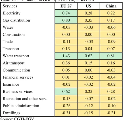
Hypothesis: EU, US, China – Full liberalization on Agriculture + Agribusiness + Industry + Services Table 2.2.1.5 – Variation on GDP by sector (%) – Services
Services EU 27 US China Electricity -0.65 0.13 0.22 Gas distribution -0.94 0.16 0.17 Water 0.01 -0.05 -0.06 Construction -0.03 0.00 0.00 Trade -0.02 -0.03 -0.09 Transport -0.07 0.01 0.07 Water transport -1.13 0.37 0.81 Air transport -0.57 0.09 0.16 Communication -0.33 -0.04 -0.03 Financial services -0.36 -0.05 -0.04 Insurance -0.14 -0.04 -0.02 Business services -0.57 0.12 0.28
Recreation and other serv. -0.03 -0.06 -0.02
Public administration 0.03 -0.08 -0.10
Dwellings 0.00 -0.12 -0.21
Simulation 1 – Brazil x EU – US – China
Hypothesis: EU, US, China – Full liberalization on Agriculture + Agribusiness + Industry + Services Table 2.2.1.6 –– GDP: Gains and losses by sector – Services
Services EU 27 US China Electricity - + + Gas distribution - + + Water + - - Construction - - - Trade - - - Transport - + + Water transport -- + + Air transport - + + Communication - - - Financial services - - - Insurance - - - Business services - + +
Recreation and other serv. - - -
Public administration + - -
Dwellings + - -
Total (No. of positive results) 3 6 6
Source: CGTI-FGV Variation on GDP (%) Classification 0 – 1 (+) or (-) 1 – 2 (++) or (--) 2 – 3 (+++) or (---) More than 3 (++++) or (----)
Simulation 1 – Brazil x EU – US – China
Hypothesis: EU, US, China – Full liberalization on Agriculture + Agribusiness + Industry + Services Table 2.2.1.7 – Summary of gains - GDP by sector
EU 27 US China Agriculture 9 17 15 Industry 1 15 12 Services 3 6 6 + 4 33 25 ++ 1 4 1 +++ 0 1 3 ++++ 8 0 4 Total 13 38 33 Source: CGTI-FGV
Table 2.2.1.8 – Macroeconomic outlook
Macroeconomic Variables EU 27 US China
Nominal GDP 1.2% -0.6% -1.2%
Real GDP 0.0% 0.0% 0.0%
Increase in total exports (US$ mi, F.O.B., 2011) 21,422 5,827 12,918
Increase in total exports % 7.8% 2.1% 4.7%
Increase in total imports (US$ mi, F.O.B., 2011) 19,502 5,496 11,807
Increase in total imports % 7.6% 2.1% 4.6%
Increase in bilateral exports (US$ mi, F.O.B., 2011) 30,996 2,537 6,100
Increase in bilateral exports % 57.9% 7.7% 12.2%
Increase in bilateral imports (US$ mi, F.O.B., 2011) 36,746 18,872 32,558
Increase in bilateral imports % 52.7% 46.2% 96.1%
Terms of trade 1.5% -0.4% -0.7%
Real wage 0.1% 0.0% 0.0%
Land gains 26.8% 2.3% 7.8%
Capital gains 0.3% 0.1% 0.2%
Real exchange rate 1.7% -0.5% -0.9%
Simulation 1 – Brazil x EU – US – China Table 2.2.1.9 – Trade Balance: Agriculture
Agriculture EU 27 US China
∆ Trade balance % % ∆ Trade balance % % ∆ Trade balance % %
(US$ Million) Exports Imports (US$ Million) Exports Imports (US$ Million) Exports Imports Paddy rice -27.70 3.81 221.53 2.90 17.14 96.61 1.81 3.13 -3.51 Wheat -299.91 282.93 13.55 11.43 2.22 51.28 10.66 11.79 -3.07 Other cereals -163.75 -10.42 12.58 7.64 0.74 0.55 3.71 3.31 9.98 Vegetables/fruits -10.91 8.79 41.71 3.47 1.64 39.63 -22.35 44.99 46.02 Oil seeds -892.18 -9.93 32.39 64.72 21.99 20.72 795.90 7.02 27.14 Sugar (cane&beet) -0.10 -30.61 27.75 0.00 0.67 0.32 -0.02 -6.39 19.58 Plant fibres -163.32 -12.30 29.43 -28.32 16.29 17.09 190.26 27.76 -4.89 Other crops (unprepared) -1144.72 -8.55 44.01 321.22 11.28 19.04 321.92 58.83 17.18 Cattle, horses, sheeps -120.57 -18.65 48.16 3.69 3.79 0.73 3.80 1.51 -1.62 Animal products -48.68 -4.08 25.14 1.05 2.06 8.54 -0.51 53.66 16.54 Raw milk -1.06 -25.13 28.96 0.06 2.44 -1.54 0.05 2.48 -1.43 Wool, silk -6.49 -32.38 24.73 0.66 4.33 -2.82 0.01 7.07 -7.10 Forestry products -2.55 -3.52 15.93 0.65 2.51 20.29 1.86 6.15 29.47 Meat: cattle, sheeps, horses 15314.88 2802.44 52.33 73.93 3.37 53.51 139.07 150.17 59.49 Meat products 7006.25 487.02 72.81 265.06 15.80 139.08 630.56 57.05 -4.92 Vegetables oils and fats -729.26 -9.32 78.07 114.50 4.13 87.03 620.79 78.58 89.81 Dairy products -138.47 59.83 175.35 -2.02 165.50 170.93 18.96 111.55 155.20 Processed rice -40.95 136.07 75.61 11.16 4.85 68.40 19.50 4.52 -3.19 Sugar 4063.15 559.62 102.22 379.89 73.44 125.82 2242.76 174.18 170.72 Food products (animal feed) 1493.67 125.28 52.46 192.86 23.02 58.40 131.06 57.77 39.15 Beverage, Tobacco products -111.77 47.85 43.09 -141.31 4.47 36.60 36.27 35.85 50.65
Simulation 1 – Brazil x EU – US – China Table 2.2.1.10 – Trade Balance: Industry
Industry EU 27 US China
∆ Trade balance % % ∆ Trade balance % % ∆ Trade balance % %
Extractive (US$ Million) Exports Imports (US$ Million) Exports Imports (US$ Million) Exports Imports Fishing -8.81 7.52 8.17 1.71 0.96 19.76 3.89 53.79 13.21 Coal 39.31 2.90 -1.56 -3.99 -0.09 -0.10 -8.48 0.01 -0.65 Oil -140.16 -1.05 0.09 80.93 1.48 -0.39 129.04 1.06 -0.61 Gas 16.26 1.12 -1.85 1.77 1.26 -0.78 -0.40 0.92 -0.08 Minerals -32.69 -0.66 1.23 51.83 0.58 1.21 160.33 1.11 5.95 Manufacturing Textiles -678.17 32.87 263.40 -102.98 48.10 271.44 -2051.29 178.32 148.14 Apparel -647.17 49.08 567.65 24.15 100.36 701.38 -1891.84 250.79 215.94 Leather products -269.92 14.64 401.70 355.71 69.49 440.79 -739.34 67.74 185.65 Wood products -224.98 3.92 138.81 12.21 8.37 128.36 -14.04 11.07 110.01 Paper products -809.49 -4.98 63.97 97.69 3.54 47.91 368.27 7.81 72.69 Petroleum products 214.53 -0.74 0.36 66.84 3.40 1.76 3.49 24.49 1.34 Chemical, rubber, plastics -4215.85 1.37 48.93 -958.14 14.14 50.56 994.08 56.21 58.73 Mineral (non-metallic) -312.23 -0.86 52.35 118.52 19.09 61.48 -169.88 89.88 62.44 Iron, steel -737.01 -3.20 64.49 244.46 5.39 79.57 274.34 14.68 68.66 Metals (non-ferrous) -284.13 6.85 55.93 277.48 5.58 70.20 510.08 11.53 92.83 Metal products -1426.66 -6.13 119.03 -355.38 6.27 143.91 -592.35 101.82 125.35 Motor vehicles and parts -2882.44 12.44 113.89 57.47 6.91 131.36 -20.92 53.05 204.03 Transport equipament -420.85 -3.80 32.14 143.69 5.55 7.57 473.07 45.49 189.62 Electronic equipment -848.65 -5.38 87.59 -122.31 6.18 87.77 -1327.23 18.31 50.64 Machinery and equipment -6836.64 -3.37 86.59 -1891.15 7.01 97.24 -2027.94 97.95 114.67 Manufactures -371.64 -6.91 139.50 -27.93 4.85 161.15 -570.76 170.54 103.90
Simulation 1 – Brazil x EU – US – China Table 1.11 – Trade Balance: Services
Services EU 27 US China
∆ Trade balance % % ∆ Trade balance % % ∆ Trade balance % %
(US$ Million) Exports Imports (US$ Million) Exports Imports (US$ Million) Exports Imports Electricity -57.62 -6.93 1.59 21.90 2.97 -1.55 43.33 5.87 -2.71 Gas distribution -3.60 -4.74 4.43 0.44 2.78 -1.48 0.90 4.68 -1.79 Water -3.88 -6.58 2.80 1.53 2.98 -2.07 3.08 6.15 -4.00 Construction -8.91 -4.19 1.99 4.24 2.37 -1.63 8.81 4.85 -2.98 Trade -166.21 -5.07 2.64 62.39 2.22 -1.68 133.17 4.57 -3.10 Transport -136.59 -3.96 2.14 57.56 1.85 -1.40 118.00 4.04 -2.84 Water transport -90.97 -3.59 0.47 43.47 1.67 -0.81 93.95 3.60 -1.46 Air transport -96.04 -3.75 1.63 40.79 1.67 -1.05 80.72 3.58 -2.17 Communication -33.61 -4.95 1.92 13.66 2.15 -1.60 27.85 4.56 -3.03 Financial services -94.10 -5.23 1.77 41.33 2.15 -1.53 81.42 4.55 -3.25 Insurance -67.71 -5.16 2.12 25.48 2.13 -1.43 52.03 4.44 -2.82 Business services -810.54 -5.01 1.86 315.76 2.15 -1.43 641.88 4.56 -2.69 Recreation and other serv. -94.63 -5.01 2.55 36.96 2.18 -1.58 77.10 4.83 -3.18 Public administration -205.91 -4.90 2.12 88.68 2.09 -1.49 174.69 4.77 -3.12 Dwellings 0.00 -0.02 5.93 0.00 0.67 -1.92 0.00 1.36 -3.66
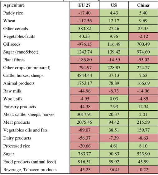
Simulation 1 – Brazil x EU – US – China
Hypothesis: EU, US, China – Full liberalization on Agriculture + Agribusiness + Industry + Services Table 1.12 – Variation on GDP by sector (US$) – Agriculture
Agriculture EU 27 US China Paddy rice -17.40 4.43 5.40 Wheat -112.56 12.17 9.69 Other cereals 383.82 27.46 25.35 Vegetables/fruits 40.23 9.76 -2.12 Oil seeds -976.15 116.49 700.49 Sugar (cane&beet) 1243.74 139.42 974.60 Plant fibres -186.80 -14.59 -55.02
Other crops (unprepared) -794.97 228.83 224.27
Cattle, horses, sheeps 4844.44 37.13 7.53
Animal products 1753.17 78.89 166.69
Raw milk -44.96 -8.73 -14.06
Wool, silk -4.95 0.03 -4.85
Forestry products -44.38 7.93 12.34
Meat: cattle, sheeps, horses 3017.91 20.37 2.01
Meat products 2075.45 94.42 215.59
Vegetables oils and fats -89.07 38.51 159.77
Dairy products -56.37 -7.39 -8.63
Processed rice -20.66 4.61 8.10
Sugar 783.77 90.83 523.90
Food products (animal feed) 916.51 59.92 45.99
Beverage, Tobacco products -45.23 -36.41 -0.22
Simulation 1 – Brazil x EU – US – China
Hypothesis: EU, US, China – Full liberalization on Agriculture + Agribusiness + Industry + Services Table 1.13 – Variation on GDP by sector (US$) – Industry
Industry EU 27 US China Extractive Fishing 10.61 0.37 0.21 Coal -1.12 0.37 0.77 Oil -147.42 62.07 116.66 Gas -3.80 1.27 2.74 Minerals -429.68 134.54 295.91 Manufacturing Textiles -497.37 -20.34 -1512.56 Apparel -217.39 15.90 -719.48 Leather products -119.17 154.99 -259.05 Wood products -181.07 13.84 -21.24 Paper products -477.58 64.31 207.77 Petroleum products -10.80 3.04 7.11
Chemical, rubber, plastics -2198.86 -300.64 497.81
Mineral (non-metallic) -185.75 52.27 -72.88
Iron, steel -1019.37 19.76 8.41
Metals (non-ferrous) -289.84 56.36 110.38
Metal products -1108.46 -203.23 -318.19
Motor vehicles and parts -802.14 44.21 46.94
Transport equipament -160.66 72.68 196.00
Electronic equipment -416.60 -52.40 -476.86
Machinery and equipment -2615.37 -559.81 -599.92
Others Manufactures -146.86 -9.54 -250.60
Simulation 1 – Brazil x EU – US – China
Hypothesis: EU, US, China – Full liberalization on Agriculture + Agribusiness + Industry + Services Table 1.14 – Variation on GDP by sector (US$) – Services
Services EU 27 US China Electricity -270.64 55.76 89.73 Gas distribution -3.81 0.66 0.68 Water 2.12 -7.46 -9.37 Construction -36.12 -4.07 -1.97 Trade -59.92 -105.22 -266.87 Transport -61.52 8.92 58.78 Water transport -107.28 35.12 77.61 Air transport -71.05 11.58 19.73 Communication -290.94 -34.56 -23.26 Financial services -453.16 -65.21 -53.74 Insurance -53.43 -14.51 -6.78 Business services -1003.97 214.84 489.49
Recreation and other serv. -16.74 -29.96 -9.51
Public administration 119.97 -369.48 -430.24
Dwellings 0.20 -174.82 -300.50
Simulation 1 – Brazil x EU – US – China Table 1.15 – Trade Balance – Agriculture
Agriculture EU 27 US China
∆ Trade balance Exports Imports ∆ Trade balance Exports Imports ∆ Trade balance Exports Imports (US$ Million) (US$ Million) (US$ Million) (US$ Million) (US$ Million) (US$ Million) (US$ Million) (US$ Million) (US$ Million) Paddy rice -27.70 1.46 0.49 -27.70 1.46 0.49 1.81 0.00 0.00 Wheat -299.91 10.44 0.12 -299.91 10.44 0.12 10.66 0.61 0.00 Other cereals -163.75 -33.46 0.02 -163.75 -33.46 0.02 3.71 0.21 0.12 Vegetables/fruits -10.91 54.01 61.90 -10.91 54.01 61.90 -22.35 0.51 67.59 Oil seeds -892.18 -257.04 0.59 -892.18 -257.04 0.59 795.90 827.50 0.17 Sugar (cane&beet) -0.10 -0.01 0.01 -0.10 -0.01 0.01 -0.02 0.00 0.00 Plant fibres -163.32 -3.35 0.17 -163.32 -3.35 0.17 190.26 167.23 0.00 Other crops (unprepared) -1144.72 -472.58 20.10 -1144.72 -472.58 20.10 321.92 261.96 2.11 Cattle, horses, sheeps -120.57 -0.05 7.69 -120.57 -0.05 7.69 3.80 0.00 0.00 Animal products -48.68 -3.26 16.43 -48.68 -3.26 16.43 -0.51 2.87 7.75 Raw milk -1.06 -0.16 0.09 -1.06 -0.16 0.09 0.05 0.01 0.00 Wool, silk -6.49 -0.13 0.01 -6.49 -0.13 0.01 0.01 0.01 0.00 Forestry products -2.55 -0.84 1.50 -2.55 -0.84 1.50 1.86 0.14 0.06 Meat: cattle, sheeps, horses 15314.88 15460.78 3.99 15314.88 15460.78 3.99 139.07 15.73 0.54 Meat products 7006.25 8118.95 19.64 7006.25 8118.95 19.64 630.56 241.79 -0.06 Vegetables oils and fats -729.26 -263.77 220.73 -729.26 -263.77 220.73 620.79 487.61 0.84 Dairy products -138.47 2.50 127.84 -138.47 2.50 127.84 18.96 1.48 3.86 Processed rice -40.95 6.75 3.33 -40.95 6.75 3.33 19.50 0.03 -0.01 Sugar 4063.15 4737.08 1.47 4063.15 4737.08 1.47 2242.76 2208.73 0.31 Food products (animal feed) 1493.67 1944.87 320.38 1493.67 1944.87 320.38 131.06 98.21 164.74 Beverage, Tobacco products -111.77 103.94 250.31 -111.77 103.94 250.31 36.27 0.95 1.11
Simulation 1 – Brazil x EU – US – China Table 1.16 – Trade Balance – Industry
Industry EU 27 US China
∆ Trade balance Exports Imports ∆ Trade balance Exports Imports ∆ Trade balance Exports Imports Extractive (US$ Million) (US$ Million) (US$ Million) (US$ Million) (US$ Million) (US$ Million) (US$ Million) (US$ Million) (US$ Million) Fishing -8.81 0.63 0.24 1.71 0.11 0.34 3.89 0.11 0.10 Coal 39.31 0.00 0.00 -3.99 0.00 -0.91 -8.48 0.00 0.00 Oil -140.16 -9.53 0.00 80.93 54.07 -0.35 129.04 19.60 0.00 Gas 16.26 0.00 -0.54 1.77 0.00 -0.41 -0.40 0.00 0.00 Minerals -32.69 -72.42 2.03 51.83 1.76 2.20 160.33 292.20 1.46 Manufacturing -2051.29 0.00 0.00 Textiles -678.17 29.31 1051.28 -102.98 58.59 577.54 -2051.29 48.12 3519.77 Apparel -647.17 29.37 978.03 24.15 52.02 127.30 -1891.84 29.59 2293.75 Leather products -269.92 171.58 353.92 355.71 260.47 50.76 -739.34 276.98 1524.34 Wood products -224.98 37.60 244.73 12.21 57.45 174.46 -14.04 6.83 282.43 Paper products -809.49 -100.47 650.40 97.69 47.76 212.87 368.27 156.43 138.53 Petroleum products 214.53 -2.35 3.07 66.84 94.92 129.32 3.49 6.37 16.34 Chemical, rubber, plastics -4215.85 46.78 6328.42 -958.14 357.93 4914.25 994.08 348.78 2462.31 Mineral (non-metallic) -312.23 -1.69 321.18 118.52 161.02 149.30 -169.88 10.58 449.89 Iron, steel -737.01 -43.33 670.07 244.46 187.27 255.91 274.34 95.95 569.35 Metals (non-ferrous) -284.13 88.14 420.93 277.48 55.68 139.81 510.08 23.12 324.44 Metal products -1426.66 -18.10 1838.26 -355.38 20.07 892.03 -592.35 24.08 1408.80 Motor vehicles and parts -2882.44 164.18 7029.41 57.47 75.54 1245.64 -20.92 40.94 2647.30 Transport equipament -420.85 -44.20 607.59 143.69 52.02 253.43 473.07 293.00 1058.14 Electronic equipment -848.65 -12.69 1108.08 -122.31 6.96 1073.01 -1327.23 14.24 3378.15 Machinery and equipment -6836.64 -65.92 13196.62 -1891.15 186.83 7944.33 -2027.94 265.60 11188.58 Manufactures -371.64 -8.22 481.39 -27.93 10.38 160.02 -570.76 70.04 922.61
Simulation 1 – Brazil x EU – US – China Table 1.17 – Trade Balance – Services
Services EU 27 US China
∆ Trade balance Exports Imports ∆ Trade balance Exports Imports ∆ Trade balance Exports Imports (US$ Million) (US$ Million) (US$ Million) (US$ Million) (US$ Million) (US$ Million) (US$ Million) (US$ Million) (US$ Million) Electricity -57.62 -3.70 23.05 21.90 0.55 -0.81 43.33 0.59 -1.67 Gas distribution -3.60 0.00 0.33 0.44 0.00 -0.04 0.90 0.00 -0.01 Water -3.88 -0.81 0.59 1.53 0.32 -0.07 3.08 0.24 -0.06 Construction -8.91 -1.39 1.54 4.24 0.00 0.00 8.81 0.00 -0.06 Trade -166.21 -24.13 46.25 62.39 3.81 -1.91 133.17 10.82 -11.53 Transport -136.59 -23.88 33.52 57.56 9.55 -1.44 118.00 7.59 -2.17 Water transport -90.97 -49.07 11.65 43.47 0.49 -0.48 93.95 0.51 -0.17 Air transport -96.04 -13.64 41.32 40.79 1.77 -5.55 80.72 1.44 -0.32 Communication -33.61 -11.73 5.06 13.66 2.11 -0.38 27.85 1.20 -0.25 Financial services -94.10 -20.12 18.53 41.33 8.15 -9.81 81.42 0.94 -0.27 Insurance -67.71 -6.59 10.80 25.48 5.25 -4.18 52.03 9.61 -1.22 Business services -810.54 -216.00 158.38 315.76 60.96 -16.42 641.88 16.85 -5.48 Recreation and other serv. -94.63 -13.30 38.02 36.96 3.63 -3.22 77.10 2.96 -1.34 Public administration -205.91 -28.37 30.98 88.68 19.58 -27.25 174.69 4.62 -1.76 Dwellings 0.00 0.00 0.00 0.00 0.00 0.00 0.00 0.00 0.00
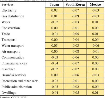
2.2.2.
Simulation 2 – Brazil x Japan – South Korea – Mexico
Hypothesis: Japan, South Korea, Mexico – Full liberalization on Agriculture + Agribusiness + Industry + Services
Table 2.2.2.1 – Variation on GDP by sector (%) – Agriculture
Agriculture Japan South Korea Mexico
Paddy rice 0.01 -0.24 -0.05 Wheat -0.02 -1.74 -0.32 Other cereals 0.78 13.93 -0.06 Vegetables/fruits 0.16 -0.35 -0.05 Oil seeds -0.02 3.15 -0.18 Sugar (cane&beet) 0.11 -0.11 0.02 Plant fibres -0.07 -0.96 -0.09
Other crops (unprepared) -0.01 -0.38 0.27
Cattle, horses, sheeps 0.02 -0.31 -0.05
Animal products 2.01 0.12 -0.15
Raw milk 0.01 -0.17 0.00
Wool, silk 2.70 -0.04 0.00
Forestry products 0.06 -0.02 -0.04
Meat: cattle, sheeps, horses 0.02 -0.39 -0.06
Meat products 3.88 0.24 -0.28
Vegetables oils and fats 0.20 -0.88 -0.12
Dairy products 0.03 -0.15 0.00
Processed rice 0.00 -0.05 -0.02
Sugar 0.19 -0.11 0.07
Food products (animal feed) 0.47 0.19 -0.01
Beverage, Tobacco products 0.05 1.19 -0.01