Design and implementation of a reliable unmanned aerial system design

(1)

Department of Information Science and Technology

Design and Implementation of a Reliable Unmanned Aerial

System Design

Tiago Miguel Simão Caria

A Dissertation presented in partial fulfillment of the Requirements for the Degree of Master in Telecommunications and Computer Engineering

Supervisor:

PhD. Pedro Joaquim Amaro Sebastião Assistant Professor at ISCTE-IUL

Co-Supervisor:

PhD. Nuno Manuel Branco Souto Assistant Professor at ISCTE-IUL

(2)

(3)

i

ABSTRACT

With the increase in popularity of the UAV, due to their high accessibility, it becomes even more important that they can be operated in a safe way not only to protect the UAV but also to protect the surroundings and the people. This thesis has the main objective to study ways that allow to increase the security of UAV operations.

We start by identifying the failures and their impact and proceed to develop a module that is independent from the principal modules of the UAV. Within this work we opted to focus on the implementation of detection and avoidance of obstacles for the MAV type of UAVs. After making an evaluation of different types of ultrasonic sensors we studied ways to connect them in an array and get a 360º cover of the UAV. Then, we developed three different implementations of an object detection algorithm, with each algorithm being a more complex version of the previous one:

First Algorithm – Detection and distance estimation from an object

Second Algorithm – Added a false alarm avoidance and direction estimation of the object

Third Algorithm – Added the ability to detect more than one object

Following the evaluation of those algorithms, we then aimed to develop an interface for the collision module which could send a message to the UAV if an object was detected so that it can change its flight mode and prevent collision. For that the MAVlink protocol was selected since it is compatible with a lot of flight controllers. In the end a final study was made in order to check what was the maximum velocity that an UAV can achieve in order for it to react in time to avoid collision.

Keywords: Unmanned Aerial Vehicles, reliable design, safety mechanics, sensors in UAV, independent module

(4)

ii

(5)

iii

RESUMO

Com o aumento na popularidade dos veículos aéreos não-tribulados, devido à sua elevada acessibilidade, torna-se cada vez mais importante quando se usa um UAV que ele esteja seguro não só para proteger o UAV mas também para proteger as pessoas e os redores de onde é usado. Esta tese tem o objetivo principal de estudar as diferentes maneiras de aumentar a segurança dos UAV quando está em uso.

Começamos por identificar as várias falhas e o seu impacto e quando terminamos isso procedemos a desenvolver um módulo que é independente do módulo principal do UAV. Com os estudos feitos optamos por focar na implementação de deteção e evitação de obstáculos e adaptar isso para os UAVs do tipo MAV. Depois da avaliação sobre os diferentes tipos de sensores ultrassónicos foi estudado várias maneiras de os ligar em sequência e conseguir uma cobertura de 360º no UAV. Depois nos desenvolvemos três diferentes implementações de um algoritmo de deteção de obstáculos, em que cada um desses algoritmos era uma versão mais complexa do anterior:

Primeiro Algoritmo – Deteção e estimação da distância de um objeto.

Segundo Algoritmo – Adição da evitação do falso alarme e estimação da direção do objeto

Terceiro Algoritmo – Adição da habilidade de detetar mais do que um objeto Após a avaliação destes algoritmos, foi desenvolvida uma interface para o módulo de evitação da colisão com obstáculos que conseguia mandar uma mensagem para o UAV para o caso em que um objeto foi detetado, para ele mudar o modo de voo e assim evitar a colisão com o obstáculo. Para isso selecionou-se o protocolo MAVlink devido à sua compatibilidade com muitos dos modos de voo. Um estudo final foi realizado de modo a verificar qual seria a velocidade máxima que um UAV poderia ter de modo a conseguir reagir a tempo e evitar a colisão.

Palavras-Chave: Veículos aéreos não-tribulados, Projeção viável, mecanismos de segurança, sensores nos Veículos aéreos não-tribulados, módulo independente.

(6)

iv

(7)

v

ACKNOWLEDGEMENTS

To my family, thanks for all the continuous support that you all gave me throughout my whole life.

I would like to also thank the Professors Nuno Souto and Pedro Sebastião for their indispensable help, being always available for help when I needed and for their advices and guidance that helped me during the course of this thesis.

A big thanks as well to IT (instituto de telecomunicações) for providing me with the materials to work on the dissertation such as arduino UNO, various different sensors and a lot more.

To Paulo Canilho, a childhood friend, for all the continuous support during all these years. I would also like to thank Bruno Ricardo, a close friend of mine, for helping me start this dissertation as it was one of the future works from his dissertation, showing me the ins and outs of it.

(8)

vi

(9)

vii

CONTENT

ABSTRACT ... i RESUMO ... iii ACKNOWLEDGEMENTS ... v CONTENT ... vii FIGURES ... xi TABLES ... xiii ACRONYMS LIST ... xv CHAPTER 1 ... 1 1.1 Overview ... 2 1.2 Motivation ... 2

1.3 State of the art ... 3

1.3.1 Critical parts in the UAV ... 3

1.3.2 Rescue System ... 4 1.3.3 Obstacle avoidance ... 5 1.4 Objectives ... 7 1.5 Contributions ... 7 1.6 Dissertation Structure ... 8 CHAPTER 2 ... 9 2.1 Overview ... 10

2.2 Unmanned Aerial Vehicles ... 10

2.2.1 Frames ... 11

2.2.2 Propulsion System ... 12

2.2.3 Electronic Speed Controller ... 12

(10)

CONTENT

viii

2.3 Payload ... 13

2.4 Launch and Recovery ... 14

2.5 Navigation System ... 14

2.5.1 Flight controller ... 15

2.5.1.1 Ardupilot ... 15

2.5.1.2 Pixhawk ... 16

2.6 Communication ... 17

2.7 Ground Control Station ... 17

2.8 Possible Failures of the System ... 18

2.8.1 Battery ... 19

2.8.2 Propulsion System ... 19

2.8.3 Sensors (Acceleration Meter; Stabilization Control; Altitude Estimation) ... 19

2.8.4 Communications ... 19

CHAPTER 3 ... 21

3.1 Overview ... 22

3.2 Overlapping Study ... 25

3.3 Connecting all the sensors together ... 29

3.3.1 – Activated Loop... 30 3.3.2 – Constantly Looping ... 30 3.3.3 – Simultaneous Activation ... 31 Chapter 4 ... 33 4.1 Introduction ... 34 4.2 Detection Algorithms ... 35 4.2.1 First Algorithm ... 35 4.2.2 Second Algorithm ... 39 4.2.3 Third Algorithm ... 43

(11)

ix 4.3 Large Distances ... 46 Chapter 5 ... 49 5.1 MavLink Packet ... 50 5.2 Flight Modes ... 51 5.2.1 Guided mode ... 51 5.2.2 Loiter ... 51 5.2.3 Position mode ... 51 5.2.4 Land Mode ... 52 5.3 MAVlink message ... 52 5.4 Testing ... 53

5.5 Maximum velocity for collision avoidance ... 55

Chapter 6 ... 57

6.1 Conclusion ... 58

6.2 Future work ... 58

(12)

x

(13)

xi

FIGURES

Figure 1 – Diagram of the UAV components. Source: (Bouabdallah et. all, 2011)... 3

Figure 2 – Implementation of the parachute. Source: (Zhaoronget al., 2013) ... 5

Figure 3 – Solution for collision avoidance. Source: (Sunberg et al., 2016)... 6

Figure 4 – Coverage of the UAV. Source: (Gageik et al., 2012) ... 6

Figure 5 – UAS Components ... 10

Figure 6 – Fixed-Wing UAV ... 11

Figure 7 – Multi-rotor UAV ... 12

Figure 8 – Propulsion System ... 12

Figure 9 – Electronic Speed Controllers... 13

Figure 10 – Battery ... 13

Figure 11 – Ardupilot Board. Source: (ArduPilot Mega, 2017) ... 15

Figure 12 – Pixhawk Board. Source: (Autopilot Hardware, 2017) ... 16

Figure 13 – Mission Planner Application. Source: (Mission Planner Overview, 2017) 18 Figure 14 – Arduino UNO. Source: (Arduino Uno Rev3) ... 23

Figure 15 – HC-SR04 connecting to an arduino device ... 23

Figure 16 – MB series sensors connected to an arduino device ... 24

Figure 17 – Range zero on the sensor marked as a red line. ... 24

Figure 18 – Representation of the symbols in Table 6 ... 27

Figure 19 – Sensor MB1260 using 8, 7 and 6 sensors ... 28

Figure 20 – Sensor MB1200 using 8, 7 and 6 sensors ... 28

Figure 21 – Sensor mb1000 using 8, 7, and 6 sensors... 28

Figure 22 – Sensor mb1020 using 12, 10, and 8 sensors... 29

Figure 23 – Sensor HCSR 04 using 12, 10 and 8 sensors. ... 29

Figure 24 – Activated loop representation ... 30

Figure 25 – Constantly looping ... 30

Figure 26 – Simultaneous Activation ... 31

Figure 27 – HC-SR04 with 3 sensors connected to arduino UNO ... 34

Figure 28 – Sensors Positions ... 35

Figure 29 – Flowchart of the First Algorithm ... 35

Figure 30 – Prints from the console of the first algorithm ... 36

(14)

FIGURES

xii

Figure 32 – Estimated distance versus real distance with one object in both sensor 1 and

3 ... 38

Figure 33 – Average value of the estimated distance versus real distance with one object in both sensor 1 and 3 ... 38

Figure 34 – Flowchart of the Second Algorithm ... 39

Figure 35 – Prints from the console of the second algorithm ... 40

Figure 36 – Object only detedted by one sensor ... 41

Figure 37 – Object detected by two sensors ... 41

Figure 38 – Detected Angle verses Real Angle ... 42

Figure 39 – Direction of an object by the algorithm ... 42

Figure 40 – Flowchart of the Third Algorithm ... 43

Figure 41 – Prints from the console of the third algorithm ... 44

Figure 42 – Difference in the measures of two sensors ... 44

Figure 43 – Estimated Angle versus Real Angle with an object moving and another stopped ... 45

Figure 44 – Estimated Angle versus Real Angle with an object moving and another stopped ... 45

Figure 45 – Estimated Distance versus Real Distances for Large distances ... 46

Figure 46 – Estimated Angle versus Real Angle with One Object and Large Distances47 Figure 47 – MAVlink packet ... 50

Figure 48 – MAVlink message to change flight mode ... 52

Figure 49 – MAVlink message to change the flight mode to loiter ... 53

Figure 50 – Connections made from arduino to APM and the APM to APM Wi-Fi ... 53

Figure 51 – Change of the flight mode from Stabilize to Loiter ... 54

(15)

xiii

TABLES

Table 1 – UAV Categories. Source: (Petricca et al., 2011) (Austin, 2010) ... 10

Table 2 – UAV components. Source: (MaxBotix Inc.. 2017) (Ultrasonic Sensor) ... 22

Table 3 – Real experiments ... 24

Table 4 – Amount of sensors needed for 1/3 and 1/2 overlap between sensors ... 26

Table 5 – Sensors needed depending on the angle of the lobe ... 26

Table 6 – Demonstration of what to expect with each sensor ... 27

Table 7 – Root mean square error for one object in one sensor ... 37

Table 8 – Root mean square error for one object in one sensor and two object in two different sensors ... 39

Table 9 – Root Mean Square Error for large distances and large objects ... 47

Table 10 – Time that it takes to change flight mode adapted from the mission planner log. ... 54

Table 11 – Delay based on the number of sensors used in chapter 3 ... 55

Table 12 – Travelled distance based on the velocity of the UAV and the maximum delay ... 56

(16)

xiv

(17)

xv

ACRONYMS LIST

3G 3rd Generation

4G 4th Generation

API Application Programming Interface ACAS Automated Collision Avoiding System APM Ardupilot Mega

ESC Electronic Speed Controllers GCS Ground Control Station GPS Global Positions System

HTOL Horizontal Take-off and Landing

ID Identifier

IMU Inertial Measurement Unit

IR Infrared

I/O Input/Output

LIDAR Light Detection and Ranging LOS Line-Of-Sight

MAV Micro Aerial Vehicle MAVlink Micro Aerial Vehicle Link

RC Radio Control

UART Universal Asynchronous Receiver/Transmitter UAS Unmanned Aerial System

UAV Unmanned Aerial Vehicle

US Ultrasonic Sensor

(18)

ACRONYMS LIST

xvi

(19)

1

CHAPTER 1

INTRODUCTION

Chapter 1 focusses on the idea behind this thesis, the motivations and objectives as well as the structure of this thesis

(20)

INTRODUCTION

2

1.1 Overview

Nowadays there is an increase in the amount of people that are starting to adopt Unmanned Aerial Vehicles (UAVs) not only for military (Cavoukian, 2012) use but also for search and rescue missions, surveillance, traffic monitoring, weather services, photography and film of hard to reach places and much more (Bekmezci et al., 2013)(

Afonso et. al., 2016).

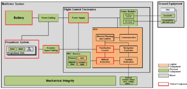
The UAV is a vehicle that is part of a complete system called UAS (Unmanned Aerial System) and being only one of the components in it (Bouabdallah et. all, 2011), there might exist failures in the different zones of the system. To establish the security of the UAV, people and of objects in the area where it is being used, this thesis will identify the failures and possible issues that have a high occurring probability (Bouabdallah et. all, 2011) during its use and develop security mechanisms to solve them.

1.2 Motivation

With the huge spike in the use of UAVs, due to their high accessibility (Chao et al., 2010), a large portion of the population has been using them not only for professional means but also for personal use. A common example would be the ability to take photos or even film places that are not easily accessible otherwise.

One of the main problems of most of the UAVs comes from the fact that for the majority of the population, Radio Control is used to communicate with the UAV since it consists of the most affordable and simple approach to establish a communication link. However, such approach cannot be undertaken in situations where there is no direct line-of-sight between the UAV and the controller (Chao et al., 2010). In the scope of the military, satellites are most commonly used to establish a communication line with the UAV. However, such approach is not viable to the wider population since it requires a significantly high budget cost.

There are a lot of problem that can occur when a UAV collides with an object that can put in risk the lives and goods in the area. Therefore, the primary aim of this thesis revolves around the idea of reducing the risk when the UAV is used when there is no

(21)

line-3

of-sight, like if it is in automated flight. Safety mechanics are also an important factor in ensuring that if something goes wrong the UAV can recover or minimize the damage done.

1.3 State of the art

There are a lot of mechanisms of security that have the objective of guarantying that UAVs are secure during their operation, both by software and hardware. In this part we are going to focus on showing the critical parts in the UAV and some of those security measures.

1.3.1 Critical parts in the UAV

To best understand how to solve those problems when there is a failure we have to first understand how does an UAV work when it comes to its components and, with that in mind we can analyse in which of them it is more possible to exist a failure in the system.

Figure 1 – Diagram of the UAV components. Source: (Bouabdallah et. all, 2011)

Figure 1 illustrates the main components that exist in a UAV. For those in a red rectangle, a failure (Battery; Power Supply; Propulsion System; Gyro; Acceleration Meter;

(22)

INTRODUCTION

4

Stabilization Control; Altitude Estimation; Actuator Signal Cabling (Bouabdallah et. all, 2011) (Valenti et al., 2006) can cause problems to the rest of the UAV. With that in mind we can then analyse and find better solutions for each case.

Regarding the communication subsystem we can observe in (Afonso et. al., 2016) how the wireless communication between the UAV and the user can be established, going in details of how to do the communication and exploring the various ways of solving the problems that can occur when there are failures in the communication. The failures at this stage can vary from problems such as latency to lack of radio coverage and one of the methods that is proposed to solve it is to implement a switching mode from automatic to manual and vice versa, so that if the communication is lost it can go on automatic mode and do an emergency landing or make it go to the last spot where it had connection and try and re-establish it.

1.3.2 Rescue System

One of the examples of a security measure for a UAV is the implementation of a parachute which can be automatically activated in the case of communication loss or even a critical failure in the UAV, as explained in (Zhaoronget al., 2013). From it we can see what are the most common occurrences for it to activate (communication lost, propeller failure), how it can be implemented and how does it work when it tries to activate it as demonstrated in Figure 2.

(23)

5

Figure 2 – Implementation of the parachute. Source: (Zhaoronget al., 2013)

There is also an important decision to make when deciding to use the parachute or any other rescue system to improve the UAVs security which is if there is a malfunction on one of the systems critical components, instead of resorting immediately to the parachute we can try to implement an emergency landing if the UAV is still operational (Fitzgerald et al., 2005).

1.3.3 Obstacle avoidance

In (Sunberg et al., 2016) we can see a proposed implementation of a proximity detection for UAVs and where it is shown the problem that currently exists when a vehicle detects an object in its way. A proposed solution to the problem resorts to dynamic programing, checking if there is a vehicle in its path and changing slightly the course to avoid collision as shown in Figure 3.

(24)

INTRODUCTION

6

Figure 3 – Solution for collision avoidance. Source: (Sunberg et al., 2016)

An additional way to get around this problem is also the use of Automated Collision Avoiding System (ACAS) (DeGarmo, 2004). With it, if there are two UAVs on the same path, each of them will hold and calculate a way to escape the collision, and as soon as they diverge from each other the control will be given back. This way a priority system can be created, for example, depending on the type of UAV.

A different approach to obstacle avoidance can be made as demonstrated in (Gageik et al., 2012) where it is shown a way to try and get a full 360º cover of the UAV.

Figure 4 – Coverage of the UAV. Source: (Gageik et al., 2012)

In Figure 4 we can then see how much sensors were used, in green the coverage of only one sensor and in yellow the coverage that overlaps between two sensors. There are a few limitation with this study since it only provides the use of a single ultrasonic sensor and the use of a fixed configuration of twelve sensors.

(25)

7

1.4 Objectives

There are some potential problems that can cause a lot of impact to the UAVs security during the operation. These problems can occur on the UAV or on the connection between the UAV and the ground control station. This thesis has the goal of reducing the occurrence of failures or even if they happen, minimize the damage.

Since the failures can happen in a lot of different parts of the system, we will identify the possible failures and classify them by relevance to try and guaranty the operability of the UAV. After that study, with the information gathered, we will try to develop an extra security module which is independent of the principal modules of the UAV. Following the information gathered we opted to focus the implementation on the problem of detection and avoidance of obstacles. Since the main target for this is the MAV type of UAV (used mostly by civilians), there will be an evaluation of adequate types of sensors, array configurations and the development of algorithms to try and detect objects with multiple beams. With that done it was an additional objective of this work to find a way to make the module compatible with different flight controllers with the use of the MAVlink protocol for the interface.

1.5 Contributions

The main contribution of this thesis is to design a module that is independent of the principal module of the UAV and helps on the detection and avoidance of obstacles, improving its security and also being compatible with the different flight modes with the use of the MAVlink protocol which is used in many different models of UAVs. The module developed is based on an array of low-cost ultrasonic sensors with simple algorithms for the detection of obstacles.

(26)

INTRODUCTION

8

1.6 Dissertation Structure

In this section we provide how the dissertation is structured and what there is in each chapter:

Chapter 1 describes the motivation and approach as well as the dissertation objectives. Chapter 2 presents an overview about Unmanned Aerial Systems (UASs) and the main components of UAVs, showing how they work in the system.

Chapter 3 focuses experiments with different sensors and how will they work once implemented on the UAV.

Chapter 4 presents the testing and results with an array of HC-SR04 sensors comprising both small and large distances for objects.

Chapter 5 explores the communication between the independent security mode and a UAV flight controller based on MAVlink messages.

(27)

9

CHAPTER 2

UNMANNED AERIAL

SYSTEMS

Chapter 2 introduces the components that make part of UAS and identifies possible failures.

(28)

UNMANNED AERIAL SYSTEMS

10

2.1 Overview

UAS are composed not only by the UAVs but also by the payload, launch and recovery, navigation system, the communication and the ground control station.

Figure 5 – UAS Components

All of the components presented in Figure 5 play an important role when using UAVs and each will be covered during this chapter showing their importance and role.

2.2 Unmanned Aerial Vehicles

Unmanned Aerial Vehicles are, by its definition, vehicles which do not require a crew to be on board to be flown. As such it can resort to either radio control or autopilot control, both of which are normally used by civilians and the military respectively.

Table 1 – UAV Categories. Source: (Petricca et al., 2011) (Austin, 2010)

Category Mass[kg] Altitude[m] Autonomy Range[km] Structure

HALE 450-13500 >15000 >Day Trans-Global Fixed-Wing MALE 450-13500 <15000 <Day 500 Fixed-Wing TUAV 15-450 <5500 <Day 100-300 Fixed-Wing Rotary-Wing

Close-range

<50 <3000 >Hour <100 Fixed-Wing Rotary-Wing Mini UAV <20 <3000 <Hour <30 Fixed-Wing

(29)

11 Rotary-Wing Micro UAV <2 <1500 <Hour <20 Fixed-Wing Rotary-Wing Nano UAV <0.025 <100 Minutes Short range Fixed-Wing

Rotary-Wing

There are a lot of different types of UAV, as showed in Table 1, but for the purpose of this dissertation the focus was on the use of the MAV type of UAV, which are the most commonly adopted amongst civilian because of its cheap price and also for its low size and weight.

In the following we will briefly describe some of the most important components in a UAV:

2.2.1 Frames

Depending on the type of UAV that is used, it can either be fixed-wings or multi-rotors. For the Fixed-wing, shown in Figure 6, they use a horizontal take-off and landing. They are more efficient for missions that are long and require heavy payload.

Figure 6 – Fixed-Wing UAV

For the Multi-rotors, shown in Figure 7, they have the rotors positioned vertically which lets them gain height in that direction. They also provide more efficiency for missions that require precise positions.

(30)

12

Figure 7 – Multi-rotor UAV

2.2.2 Propulsion System

The propulsion system, illustrated in Figure 8, is responsible for generating force that moves the UAV, with it being a combination of actuators (motors and propellers), which can be positioned differently depending on the type of frame chosen, and the Electronic Speed Controllers (ESC).

Figure 8 – Propulsion System

2.2.3 Electronic Speed Controller

Electronic Speed Controllers (ESC), presented in Figure 9, has the main responsibility of receiving the information from the flight controller and transmit all the commands to the vehicles motors.

(31)

13

Figure 9 – Electronic Speed Controllers

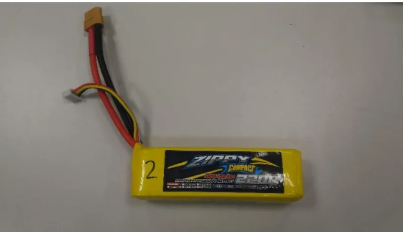
2.2.4 Battery

The battery, Figure 10, is one of the most important components in the UAV since it is required for it to have power to operate. Depending on the type of UAV we are using it can last from a few minutes to days. The battery in combination with the ESC and the actuators must be dimensioned in order to attain maximum efficiency.

Figure 10 – Battery

2.3 Payload

The payload represents the weight of all of the things that are in the UAV but are not important for its functionality, which also includes safety mechanism like the parachute. One of the main priorities when adding payload to the UAV is to ensure that it maintain its stability when flying (Pounds et al., 2012).

(32)

14

Depending on the mission that the UAV is designed to do, it can vary from a lot of things (Puri, 2005). For example, the amount of payload that a mission, such as recording a video at a difficult place to reach, takes is significantly lower than of a mission that requires the UAV to transport an object to a specific location.

2.4 Launch and Recovery

There are two types of ways to perform the launch, namely, the vertical take-off and landing (VTOL) or the horizontal take-off and landing (HTOL).

VTOL vehicles, such as rotating wing aircrafts, can perform the launch and landing the same way, they also require a small space, of the size of their diameter, to perform it. HTOL vehicles, such as the fixed wings, are different from the VOTL since they need a bigger space to perform their landing and launching as they are required to run along a track.

For the recovery part, if the UAV is on manual mode then it can be done with the security measures that are implemented in it like the parachute. For the automatic mode, with the assist of a GPS it can go to the specific place where it was originally going or it can perform an automated landing.

2.5 Navigation System

The navigation system is an important part of the UAV since with it, the GCS can know where the UAV is at any given time and with that a decision can be made on where it should go next. If the UAV is on autopilot, it can try to automatically calculate where to go.

The Global Positions System (GPS) is an important part of the navigation system since it gives updates of the area and where is the UAV position, letting us control it from a distance. There are also other important sensors that help with the navigation, that are part of the Inertial Measurement Unit (IMU) such as the gyroscope, to measure angular rates

(33)

15

to guaranty that the UAV is stable, the accelerometer, to calculate linear acceleration and speed of the UAV, and magnetometer, to show the cardinal direction of the UAV. With the help of systems like the GPS and the other sensors equipped on the UAV, there can also be given a better understanding of the area around the UAV during its use (Cesetti et al., 2010).

2.5.1 Flight controller

Flight controllers are basically a way to control the UAV by connecting to it via a link system which allows them to send information and positioning from the GCS. There are a lot of different flight controllers available but we are focusing in two of the most common open-source ones.

2.5.1.1 Ardupilot

The Ardupilot is an autopilot based on the arduino platform (Bin & Justice, 2009). This flight controller can be used for controlling several different types of vehicles, from ground rovers to helicopters.

(34)

16

Ardupilot is divided into three main components:

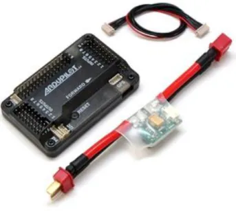
 APM Hardware – the physical board (Figure 11)

 APM Firmware – the code that runs on the board

 APM Software – the program that runs in the PC

A few strengths of ardupilot is the fact it can be easily connect to Xbee modules which is a two way telemetry that is used for wireless communication, it has a navigation system based on GPS waypoints an it has an autonomous stabilisation granted by the build-in hardware failsafe. Also being open-source it has the ability to be constantly updated and improved over time.

2.5.1.2 Pixhawk

PixHawk is an open source project with a high end autopilot hardware that has a low cost. The Pixhawk is divided into two main factors, the software and hardware. The hardware is compound by the pixhawk board showed in Figure 12 with a 168 MHz Cortex M4F CPU, 4 sensors, an integrated failsafe processor and slots for microSD, I2C, etc. (Autopilot Hardware, 2017).

(35)

17

For the software it supports PX4 and APM. For the PX4 it has both the functionalities of the PX4FMU (Flight Management Unit) that is responsible for the information in the sensor and the PX4IO (input/output) which is responsible for the input and output of the information.

2.6 Communication

For the communication between the GCS and the UAV it can be done either by radio control links, which requires LOS, or by wire-less communication technologies like 3G, 4G, Wi-Fi or satellite.

The radio control is used by most common civilian UAVs since it is the cheapest option but requires LOS operation in order to work or there will be connection lost. For the wireless version, only the satellite option is restricted for military use, while the other wireless communication technologies are open to everyone but due to the high cost for it to be used and implemented in a UAV it is still not common on civilian vehicles.

The uplink, which is the communication from the GCS and the UAV, is used to send command information to the UAV such as intended position or direction while the downlink, which is the communication from the UAV to the GCS, can send general telemetry, images, battery levels or other useful information (Herwitz et al., 2004). One of the examples of a protocol that can be used for the communications between the UAV and the GCS is the MAVLink protocol which is a header-only message protocol which works well with micro UAVs and is adopted by both PIXHAWK and APM flight controllers presented in section 2.5.1.

2.7 Ground Control Station

The Ground Control Station (GCS) is the one responsible for controlling the UAV. Depending on the flight mode, the UAV can either be manually controlled during the whole flight or autonomously by selecting waypoints we want the UAV to reach (Berni

(36)

18

et al., 2009). The other devices that exist in the UAV, such as camera, can also be controlled by the GCS (Jovanovic & Starcevic, 2008).

The GCS sends its controls to the UAV by the uplink where it commands it to move to specific places or directions. It is also the receiving end of a lot of information from the UAV by receiving information relevant to it by the downlink. By having the information of the UAV and of the surroundings it is also important to check if there is a problem with the UAV during the use or in a specific mission so that it can avoid unnecessary damages to it.

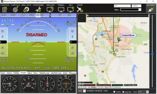
One example of a GCS is the Mission Planner, shown in Figure 13, which is an open source GCS application compatible with the MAVlink protocol which lets us monitor various values from the UAV as well as control it.

Figure 13 – Mission Planner Application. Source: (Mission Planner Overview, 2017)

2.8 Possible Failures of the System

There are a lot of possible failures that can happen during the use of the UAV. In this sections we present some of the most important components or group of components where a failure can have a negative impact on both the UAV and the environment where it is used.

(37)

19

2.8.1 Battery

For the battery since it is one of the most important components in the UAV, a failure here can make the UAV stop working since for most of the components in the UAV it is the main source of power.

2.8.2 Propulsion System

The propulsion System is responsible for the movement of the UAV. Were to happen a failure in it, depending on the type of structure that the UAV presents, the control over the UAV can either be totally lost or it can still fly with less stabilization until the loss of the stabilization.

2.8.3 Sensors (Acceleration Meter; Stabilization Control;

Altitude Estimation)

In the case that there is a wrong reading by any of the sensors, some information may be taken differently than intended which may cause the GCS to take different decisions based on those reading that the UAV sends or it may cause some systems in the UAV to react differently.

2.8.4 Communications

The loss of communication between the UAV and the GCS presents a threat, especially when the UAV is not controlled by wireless communications, the loss of LOS can present a problem without any way of re-establishing the connection or any mechanism to stop the UAV from falling.

(38)

20

(39)

21

CHAPTER 3

LOW COST DISTANCE

MEASUREMENT

SENSORS FOR UAV

Chapter 3 shows the study done regarding the ultrasonic sensors and a way to implement them in the UAV.

(40)

LOW COST DISTANCE MEASUREMENT SENSORS FOR UAV

22

3.1 Overview

The main objective behind this chapter is to develop an extra security measure that is independent of the main modules of the UAV. Therefore we focussed on implementing a means of detection and avoidance of objects for the MAV type of UAV while making sure it covers the UAV as a whole (360º). With that we looked at the different types of available sensors and decided to go for the ultrasonic sensors (US). Other options were considered like infrared sensors (IR) and Light Detection and Ranging sensors (LIDAR). However besides having a lower cost compared to the other two, US are reliable than IR sensors since they are not affected by the different light and colour conditions (Adarsh et al., 2016) and weight less than LIDAR sensors.

We start by checking the datasheets from different modules and manufactures and came to the conclusion presented in Table 2:

Table 2 – UAV components. Source: (MaxBotix Inc.. 2017) (Ultrasonic Sensor)

To see how the sensors will perform in a real scale environment they were put to test to see the max amount of range they have and the max beamwidth they can achieve. For the tests that we are going to conduct we will be using Arduino which is an open source electronic platform that comes both with a board and a software that lets us test sensors and other devices.

Sensor Price Max range Lobe

MB1000 29.95$ 6.45m ~60º

MB1020 29.95$ 6.45m ~38º

HC-SR04 3,95$ ~5m ~30º

MB1260 54.95$ 10.65m ~60º

(41)

23

Figure 14 – Arduino UNO. Source: (Arduino Uno Rev3)

With the Arduino UNO (Figure 14) and using both the HC-SR04 and the MB1260 sensors we decided to test how the sensors preformed in a real scenario and made the connections showed in Figure 15 and Figure 16.

(42)

24

Figure 16 – MB series sensors connected to an arduino device

Using a ruler and a protractor and stating the reading on the range zero (Figure 17) of the sensor we got the results on Table 3.

Figure 17 – Range zero on the sensor marked as a red line. Table 3 – Real experiments

Sensor Max Range Measured (m) Max Range Datasheet (m)

HC-SR04 4.80 ~5m

MB1260 9.75 10.65

With the results we got from the real experiments we can see that the HC-SR04 is a little bit off the datasheet value while the MB1260 is almost one meter away from the datasheet value. There are many factors that might have influenced the results but one of the main

PW

MB Series

(43)

25

reasons might be the bigger the distance becomes, the less accurate we can predict the max value. This is going to be covered in chapter 4

3.2 Overlapping Study

Since our objective is to get a full scale cover of the UAV (360º) there are some calculations we had to perform in order to get the minimum amount of sensors need to accomplish that. The next function gives the number of sensors that we need in order to achieve that goal:

𝑁𝑠 = 360º + 𝑦 × 360º

𝑥 (1)

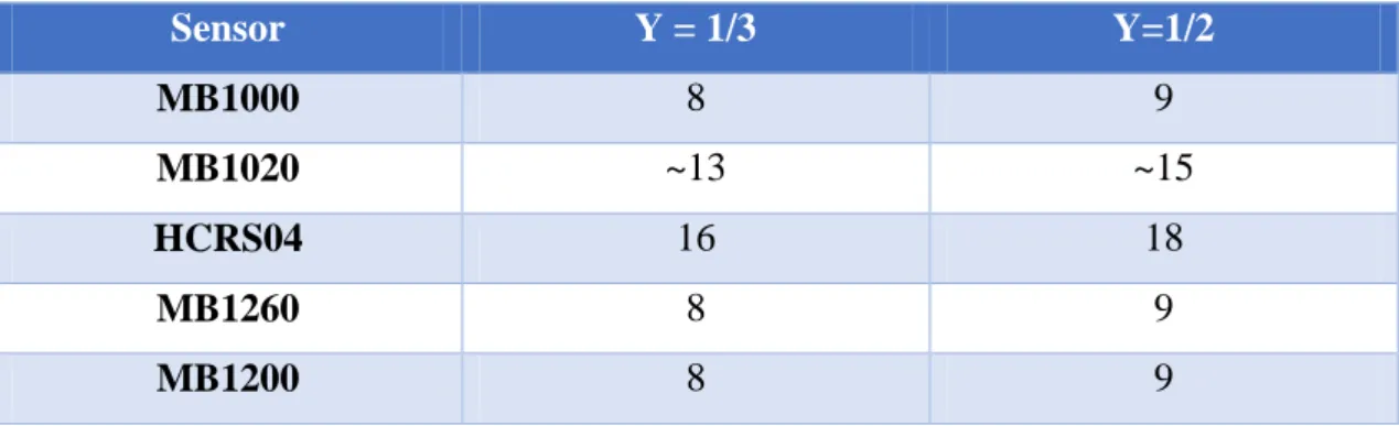
In which x is the angle of the lobe of our sensor and y is the percentage of the lobes of two sensors overlapping each other, meaning that if we want to use a sensor with a lobe angle of 60º and the overlap between two sensors is 1/3 then we would need 8 sensors to reach that goal.

𝑁𝑠 = 360º + 1

3 × 360º

60º = 8

For the sensors used in the study we made a table (Table 4) with the number of sensors required to obtain an overlap of 1/3 and 1/2:

(44)

26

Table 4 – Amount of sensors needed for 1/3 and 1/2 overlap between sensors

Sensor Y = 1/3 Y=1/2 MB1000 8 9 MB1020 ~13 ~15 HCRS04 16 18 MB1260 8 9 MB1200 8 9

After the study on the different sensors we decided to make a more generic approach and see how many sensors will be needed depending on the lobe of the sensor (from 20º to 60º) and the different values of lobe overlapping between sensors (from 1/5 to 1/2). The results are shown in Table 5. In the case that it wasn’t an integer number we round it up so that we can get the exact number of sensors needed for the overlap value we want which means that for some values of overlapping there can be the same amount of sensors required.

Table 5 – Sensors needed depending on the angle of the lobe

X(º) Y = 1/5 Y = 1/4 Y = 1/3 Y=1/2 60 8 8 8 9 50 9 9 10 11 40 11 12 12 14 30 15 15 16 18 20 22 23 24 27

Following that, Table 6 focuses on showing the results we can expect from the different sensors used in this study based on the amount of sensors used, from 6 to 16 sensors.

(45)

27

Table 6 – Demonstration of what to expect with each sensor Nº of sensors Angle (º) α (θ = 30º) γ (θ = 30º) α (θ = 38º) γ (θ = 38º) α (θ = 60º) γ (θ = 60º) 16 22,5 15 7,5 7 15,5 0 30 15 24 18 6 10 14 0 30 14 25,7 21,4 4,3 13,4 12,3 0 30 13 27,7 25,4 2,3 17,4 10,3 0 30 12 30 30 0 22 8 0 30 11 32,7 30 0 27,5 5,3 5,5 27,3 10 36 30 0 34 2 12 24 9 40 30 0 38 0 20 20 8 45 30 0 38 0 30 15 7 51,4 30 0 38 0 42,9 8,6 6 60 30 0 38 0 60 0

In Table 6 we can see different symbols which represents the following attributes: θ = represents the angle of the lobe of the sensor

α = represents the angle of the lobe without the overlap of the other sensors

γ = represents the amount of overlapping there is between two sensors

The definition of these angles is illustrated in Figure 18.

(46)

28

Using both studies we can see in the next figures how each sensor will work with some examples. All the images where made using the lobes presented in the datasheet of each sensor. They are not in scale and the amount of sensors used for the figures differs based on the angle of the lobe of each sensor.

Figure 19 – Sensor MB1260 using 8, 7 and 6 sensors

Figure 20 – Sensor MB1200 using 8, 7 and 6 sensors

(47)

29

Figure 22 – Sensor mb1020 using 12, 10, and 8 sensors.

Figure 23 – Sensor HCSR 04 using 12, 10 and 8 sensors.

In blue we can also see how much the overlap will be. As expected, the more sensors we use the more overlap we will get. In addition, the more overlap they get the more precise we can detect the object since we know more specifically in which direction it is.

3.3 Connecting all the sensors together

To connect all the sensors together there are a lot of ways to do it. However we are only focusing on three of them which are the most beneficial for the intention of this dissertation. Also depending on the method used there are smalls changes that need to be made in the code and/or in the connections.

(48)

30

3.3.1 – Activated Loop

The first one has the sensors connected in sequence and each sensor performs the calculation one by one. When all sensors finished their calculations it only triggers again once the operator commands it like showed in Figure 24.

Figure 24 – Activated loop representation

3.3.2 – Constantly Looping

The next one is just like the Activated Loop one but instead of having to trigger it to do the calculations of all the sensors, it will always be on loop, so when it goes throw all the sensors it will start again from the beginning, like shown in Figure 25.

(49)

31

3.3.3 – Simultaneous Activation

On the last one all of the sensors trigger at the same time and do the calculations needed to see the object, stopping until there is another trigger as shown in Figure 26. Sometimes this method can have a few problems with miss calculations depending on the way the sensors are positioned.

(50)

32

(51)

33

Chapter 4

LOW COMPLEXITY

OBSTACLE DETECTION

ALGORITHMS

Chapter 4 shows the results of testing the sensor array with different algorithms.

(52)

LOW COMPLEXITY OBSTACLE DETECTION ALGORITHMS

34

4.1 Introduction

After the study made on the sensors in Chapter 3 we then proceed to test how the sensors will perform in an array and with different algorithms for the detection of objects. In order to test it, we used an array of three sensors (HC-SR04) connected to the Arduino UNO as demonstrated in Figure 27, and evaluated the behaviour of three different algorithms for the detection of objects.

Figure 27 – HC-SR04 with 3 sensors connected to arduino UNO

For the tests, there was also a small delay of 50ms between each sensor triggering for the sensor to properly detect the real distance between the object and the UAV since there is a problem when all the sensors make the calculations at the same time as explained in 3.3.3. There is also a way to detect in which angle the object is, in the case of the example we have only three sensors so it will be between 330º and 30º like showed in Figure 28.

(53)

35

Figure 28 – Sensors Positions

4.2 Detection Algorithms

4.2.1 First Algorithm

For this first algorithm we made it as simple as possible so that it scans for an object and if it detects one it shows the distance, as demonstrated in Figure 29.

Figure 29 – Flowchart of the First Algorithm

During the tests, we made it so that the maximum distance was between 84 cm and 90 cm and anything below that value was considered as an object detected. Also for the prints

(54)

36

from the console it was made so that it always prints the distance so that we can see any difference. In Figure 30, from left to right, we can see various prints from the console where it shows how the algorithm detects an object.

Figure 30 – Prints from the console of the first algorithm

After testing the sensors with the distances we then made it so that we keep track of the sensors distance and see how off it was from the real distance. With a single object starting at 20cm and going all the way to 90cm, moving it 5cm each time we got the following results in Figure 31.

0 Objects 1 Object in sensors 2 and 3

1 Object in

(55)

37

Figure 31 – Estimated distance versus real distance with one object

For one object we made the same test five times and calculated the root mean square error, presented in Table 7, to see how much off the measured distance was from the real distance. It was around 0,79cm of a difference which is a good result, being really close to the real value.

Table 7 – Root mean square error for one object in one sensor

Afterwards we made it so that we have an object on both sensor 1 and 3 and made the same test as the previous one just to see the accuracy again with two sensor at the same time and got the results on Figure 32 for all the tests and in Figure 33 for the averages of both sensors in each test.

0 10 20 30 40 50 60 70 80 90 100 20 25 30 35 40 45 50 55 60 65 70 75 80 85 90 Es timated Dis ta n ce (c m ) Real Distance (cm)

Low Distances One Object

1st Measurements 2nd Measurements 3rd Measurements 4th Measurements 5th Measurements Real Distance One Object Root Mean Square Error 0,791623

(56)

38

Figure 32 – Estimated distance versus real distance with one object in both sensor 1 and 3

Figure 33 – Average value of the estimated distance versus real distance with one object in both sensor 1 and 3

For both Figure 32 and Figure 33 we can see that once again it detects the object and its distance is close to the real value. Comparing the root mean square of both test we get the following results presented in Table 8.

0 10 20 30 40 50 60 70 80 90 100 20 25 30 35 40 45 50 55 60 65 70 75 80 85 90 Es timated Dis ta n ce (c m ) Real Distance (cm)

First Algorithm One Object in Both Sensor 1 and

3

Sensor 1 Test 1 Sensor 3 Test 1 Sensor 1 Test 2 Sensor 3 Test 2 Sensor 1 Test 3 Sensor 3 Test 3 Sensor 1 Test 4 Sensor 3 Test 4 Real Distance 0 10 20 30 40 50 60 70 80 90 100 20 25 30 35 40 45 50 55 60 65 70 75 80 85 90 Es timated Dis ta n ce (c m ) Real Distance (cm)

First Algorith One Object in Both Sensor 1 and 3

Average

Average Test 1 Average Test 2 Average Test 3 Average Test 4 Real Distance

(57)

39

Table 8 – Root mean square error for one object in one sensor and two object in two different sensors

We got a value around 0,791623 for the case of one object and one sensor and then for the case of one object in two sensors we got a value around 0,877971. So in theory we can expect an offset of around 1cm for distances around 1m.

4.2.2 Second Algorithm

Following the initial idea of the first algorithm, it was time for it to become more complex so we added the estimation of the direction of the object and also added a temporal window, which can have a length of two or more periods, to filter when it detects an object in order to reducing the chance to get a false alarm from one of the sensors. For the tests we opted for the temporal window to be of the value of two periods as presented in Figure 34.

Figure 34 – Flowchart of the Second Algorithm

One Object and one sensor One Object in sensors 1 and 3

(58)

40

Using this second algorithm some detection examples are presented in Figure 35 where we can see that on the left print it was detected an object on two of the sensors (sensor 2 and 3), saying that the object was between them and on the right it was detected an object on all the sensors which means the object was mostly centred in sensor 2. For both the prints we can also see that it didn’t print where the object was situated until it was detected two times so that it avoids false alarms.

Figure 35 – Prints from the console of the second algorithm

With the results from this test we are able to predict in which direction the object is and also prevent the problem that can happen with a false alarm because it needs to detect the object two times in a row.

To calculate the direction of the object, we made it so that if an object is detected by one sensor only, like demonstrated in Figure 36, then we can assume that the direction that sensor is facing is where the object is situated. For the case that it is detected by two sensors, like showed in Figure 37, then we can assume that the object is between the two sensors detected.

Object detected in 2 and 3

Object detected in all 3 sensors

(59)

41

Figure 36 – Object only detedted by one sensor

Figure 37 – Object detected by two sensors

To test the effectiveness of the algorithm when estimating the direction of the object, an object was placed at -30º and moved 5º each time until it reached 30º. Figure 38 presents the results of this test.

(60)

42

Figure 38 – Detected Angle verses Real Angle

As we can see in Figure 38, the values from detected angle are similar to the results of the real angle. The maximum difference from the real value is 15º which happens because of the way the algorithm is designed since it can only detect angles from 15º to 15º as showed in Figure 39, where the yellow square represents the object and in that square there is a value which is the value the algorithm gives depending on the position of the object.

Figure 39 – Direction of an object by the algorithm

-40 -30 -20 -10 0 10 20 30 40 -30 -25 -20 -15 -10 -5 0 5 10 15 20 25 30 Es timated An gle (º)

Real Angle of the Moving Object (º)

Second Algorithm One Object

Detected Angle Real Angle

(61)

43

4.2.3 Third Algorithm

A third version of the algorithm was developed which had the additional ability to see if there are two objects instead of only one. The respective flowchart is shown in Figure 40.

Figure 40 – Flowchart of the Third Algorithm

The main idea behind the additional functionality is to check if there are two objects. For that we check if the distance from the two sensors that are adjacent is more than thirty centimetres and if that is the case then the algorithm decides that there is more than one object detected. If there is an object detected on two sensors that are not adjacent then it also assumes that there are two objects. An example is shown Figure 41.

(62)

44

Figure 41 – Prints from the console of the third algorithm

The reason behind choosing the value of at least thirty centimetres for the two objects detection was due to the fact that during our tests we noticed that when we have an object in a diagonal position and being detected by two sensors, as demonstrated in Figure 42, the difference in distance from the two sensors was around twenty to twenty five centimetres.

Figure 42 – Difference in the measures of two sensors

2 objects detected in sensor 1 and 3

2 objects detected in sensor 1 and 2

(63)

45

For the tests involving two objects we made it so that we always have one of the objects move 5º between detections while the other one is stopped in one place the whole time. There is also a difference of more than 30cm between them so that it detects them as two objects.

Figure 43 – Estimated Angle versus Real Angle with an object moving and another stopped

Figure 44 – Estimated Angle versus Real Angle with an object moving and another stopped

In Figure 44 the object was stopped at 0º and for Figure 43 we got the object stopped at 30º. As we can see on both examples we get results close to the real value. The main

-40 -30 -20 -10 0 10 20 30 40 -30 -25 -20 -15 -10 -5 0 5 10 15 20 25 30 Es timated An gle (º)

Third Algorithm Two Objects

Detected Angle 1 Detected Angle 2 -40 -30 -20 -10 0 10 20 30 40 -30 -25 -20 -15 -10 -5 0 5 10 15 20 25 30 Es timated An gle (º)

Third Algorithm Two Objects

Detected Angle 1 Detected Angle 2

(64)

46

difference occurs when both objects are detected by the same sensor. Since it can’t decide if there are two objects or not, it detects it as a single object, as shown in both Figure 43 and Figure 44.

4.3 Large Distances

After we did the tests for the three algorithms we then decided to try the last algorithm for large distances, where we have a big object, starting in 200cm and go until 425cm, adding 25cm with each measurement. The use of a big object comes to the fact that for the large distances it is hard for the sensor to detect small objects or even people. The results are presented in Figure 45.

Figure 45 – Estimated Distance versus Real Distances for Large distances

With the results of Figure 45 and comparing it to the results we got on section 4.2 we can see that even though there is a difference in the estimated value compared to the real value it is not that far off the real value. Afterwards making the tests we calculated, like we did in section 4.2, the root mean square error, getting the following results in Table 9.

175 200 225 250 275 300 325 350 375 400 425 450 200 225 250 275 300 325 350 375 400 425 Es timated Dis ta n ce (c m ) Real Distance (cm)

Large Distances One Object

1st Measurements 2nd Measurements 3rd Measurements 4th Measurements Real Distance

(65)

47

Table 9 – Root Mean Square Error for large distances and large objects

So in general we are looking at around a 4cm to 5cm difference from the original value which is to be expected as we get further away from the sensor the more the value of root mean square error will be.

Another detail that was detected while testing objects at large distances is that, once we get near 400cm and after that point, we start to get some errors where sometimes it doesn’t detect that the object is out of range which can be caused by reaching the maximum range of the sensor.

For the estimation of angular position of the object we did the same thing we did in section 4.2 but this time we did it for large distances and large objects and got the results presented in Figure 46.

Figure 46 – Estimated Angle versus Real Angle with One Object and Large Distances

With this results for the big distances we can see that we get a little better results than the ones in section 4.2 since the maximum difference from the estimated value and the real

-40 -30 -20 -10 0 10 20 30 40 -30 -25 -20 -15 -10 -5 0 5 10 15 20 25 30 Es timated An gle (º) Real Angle (º)

One Object Large Distances

Detected Angle Real Angle

One Object Root Mean Square Error 4,318565

(66)

48

value is 10º while in section 4.2 it is 15º. The reason behind that could be that with large objects it gets detected more easily by two sensors and since we can only detect from 15º to 15º we get a more realistic measure of the angle.

(67)

49

Chapter 5

SENSOR ARRAY

COMMUNICATI

ON INTERFACE

Chapter 5 focusses on the MAVlink protocol, the different flight modes and connections to the GCS

(68)

SENSOR ARRAY COMMUNICATION INTERFACE

50

After doing the study of the array of sensors we wanted to have a way for the independent obstacle detection block to communicate with the UAV. We decided to use the MAVlink protocol which is a header-only message protocol that works great for the type of UAV we are using and it is compatible with many different flight controllers.

5.1 MavLink Packet

In Figure 47 it can be seen how the MAVlink packet is built. Firstly we get the Packet start sign which dictates the start of a new packet and has the value of 0xFE (in version 1.0). The following five fields can have values between 0 and 255 with the exception of the System ID which has a minimum value of 1. Starting with the payload length which indicates the length of the payload. The packet sequence lets the protocol know how the sequence of the messages between it and the UAV are and if they are in order or if there is a packet loss. For the System ID it allows to choose which UAV it is sending the message. With the component ID it lets the sender choose which components to target in the UAV which is really useful for flight modes. The message ID defines what the payload means and how to decode it. The payload contains the data of the message with a value between 0 and 255 bytes. Lastly the checksum which has two bytes and is calculated based on the information that came before it, except the message ID and the data, and secures the integrity of the message. The minimum packet length is 8 bytes which corresponds to only an acknowledge while the maximum is 263 bytes with a full payload.

(69)

51

5.2 Flight Modes

There are a lot of flight mode defined in the MAVlink protocol but we are only going to focus on four of them for the purpose of the objectives of this work which ultimately aims to avoid a collision and safeguard the vehicle.

5.2.1 Guided mode

With the guided mode we get the functionality to move the UAV into a specific position. When it arrives to the target position it will hover over that location until another order is given. For this specific mode we have to use a ground station application like the Mission Planner which allows us to select a specific place for the UAV to move as a point-and-click entry.

5.2.2 Loiter

The main focus of the loiter mode is to stop the vehicle in the air while maintaining its position and altitude. In this mode the user can still control the UAV as if there was no mode activated but when the user stops giving any input it simply stands in the air while waiting for another input.

5.2.3 Position mode

Just like the loiter mode, this mode works the same way with a caveat: instead of locking everything, the position mode allows the user to control the UAV with a manual throttle and with that the user can control the UAV while it maintains a consistent positioning.

(70)

52

5.2.4 Land Mode

The land mode commands the UAV to perform a horizontal landing with a few extra characteristics, depending on the altitude of the UAV the speed at which it goes down is decreased as it comes closer to landing and that can be achieved with the help of the Altitude Hold controller. Once it lands it will shut down automatically.

5.3 MAVlink message

In this chapter we are going to explore the different messages that can happen between the UAV and the GSC. Of all the flight modes that we presented in the first part of this chapter we are going to focus on the loiter mode since that is the one that comes close to what we want to do in case there is an obstacle detected in the path of the UAV.

Figure 48 – MAVlink message to change flight mode

In Figure 48, we present the structure of the message to change the flight mode. Following the official documentation provided by ArduPilot (MAVLink Routing in ArduPilot, 2017), the “system_id” of the GCS corresponds to the number 255 and “target_system” (also referred as vehicle) to the number 1. The “component_id” parameter is used to specify whether the message sent should be broadcasted to all systems or components. Since only one system was used, this parameter is set to 0 so that all components that correspond to the previously specified “system_id” receive the message. The parameter “msg” corresponds to an internal object of the ArduPilot API that is used as a storage repository for the compressed contents of the message to be sent. Due to the lack of documentation supplied by the ArduPilot API for the parameter corresponding to the “base_mode”, we followed approaches found in academic projects that shared similar objectives/goals to the one of this system. Using such approach, we used the number 1 for this parameter. The last and most important parameter, named “custom_mode”, corresponds to the flight mode. The number used in this parameter follows the

(71)

53

specification supplied in (Github, 2017) and can be dynamically changed depending on what flight mode we desire to choose for the UAV. In this project, the loiter mode was chosen (which corresponds to the number 5). With all of this we get the final result for the message in Figure 49.

Figure 49 – MAVlink message to change the flight mode to loiter

5.4 Testing

To simplify the implementation, we have only three sensors active on the direction the sensor is facing, since this information can be obtained in a MAVlink message from the flight controller.

Figure 50 – Connections made from arduino to APM and the APM to APM Wi-Fi

For the implementation we connected arduino UNO to the APM using the UART0, as shown in Figure 50, and configured it so that a message is sent to change the flight mode to loiter as soon as an object is detected. To check also if there was a flight mode change we connected the APM to the computer by Wi-Fi and connected it to the mission planner

(72)

54

software. We chose to use a Wi-Fi connection because once we connect the APM to the computer with USB it rejects any other message from the UART0.

Figure 51 – Change of the flight mode from Stabilize to Loiter

As we can see in Figure 51, the flight mode was changed from stabilize to loiter, as identified in the white rectangles since it detected an object and the message was sent. After that implementation we decided to check how long it will take for the obstacle detection module to instruct the flight controller to change to loiter mode. Since we use only three sensors and having an object appear at the start of a detection cycle it will take 150ms (small delay of 50ms that was implemented between each sensor in order to get better accuracy) to go throw the three sensors to see if there is an object. After that, if an object is detected, a message is sent to the APM in order to change the flight mode. Once in the APM it will take approximately 1000ms for it to change its flight mode as we can see in Figure 52 and in Table 10 which show the flight mode changing from stabilize to loiter.

Table 10 – Time that it takes to change flight mode adapted from the mission planner log. Time Flight Mode Enumeration Number

15:57:53.732 Stabilize 0

(73)

55

Figure 52 – Instant of the graph it changes the flight mode presented in Table 10

Therefore we came to the conclusion that it will take around 1150ms for the UAV to react as a whole to the appearance of an object and changing the flight mode. This time can be higher in the case where more sensors are active as this adds an additional delay of 50ms for each extra sensor that is used. With the amount of sensors that can be used in the array and which were discussed in chapter 3 for the different sensors we can see in Table 11 the amount of delay there would be in total.

Table 11 – Delay based on the number of sensors used in chapter 3 Number of sensors Delay(ms)

6 300

7 350

8 400

10 500

12 600

5.5 Maximum velocity for collision avoidance

Taking into account the measured delays we then proceeded to see how the UAV will perform when it detects an object depending on the velocity it has and what might be its maximum safe velocity that allows it to detect an object and still avoid a collision. First we decided to see what was the distance travelled by an UAV based on the total delay between obstacle detection and command execution and the velocity it has. Using