Instituto Politécnico de Leiria Escola Superior de Tecnologia e Gestão
Robotics Department Masters in Eletrical Engineering
A N A LY S I S O F A N R G B D C A M E R A F O R M A N H O L E I N S P E C T I O N
Instituto Politécnico de Leiria Escola Superior de Tecnologia e Gestão
Robotics Department Masters in Eletrical Engineering
A N A LY S I S O F A N R G B D C A M E R A F O R M A N H O L E I N S P E C T I O N
f i l i p e c a s ta n h e i r a j o rg e
Project developed under supervision of Doctor Hugo Costelha([email protected])
A B S T R A C T
As the service life of ducts and manholes reaches their end, there is a growing need to preserve the structures. In order to prevent casualties and service interruption, more frequent inspections are advised. To this day most of the inspections are still, manually made. These inspectors need to be highly qualified, and the inspections are done in an hazardous environment so, automating the inspection process would lead to a healthier workplace. Given the recent development in RGBD cameras, with smaller size factor, cost, and weight, this project aims to evaluate the application of one of the more recent models in a manhole inspection environment. Several analysis are done to assess the RGBD sensor performance for 3D model reconstruction, including the comparison with a ground-truth 3D model obtained using a laser point profile sensor with an industrial robot.
C O N T E N T S
Abstract i
Contents iii
List of Figures v
List of Tables ix
List of Abbreviations and Acronyms xi
1 i n t ro d u c t i o n 1
2 s tat e o f t h e a rt r e l at e d wo r k 5
2.1 Road tunnel inspection using a Mobile Robot . . . 6
2.2 Rail-based Duct Inspections . . . 7
2.3 Tunnel inspection using an Airborne Vehicle . . . 9
2.4 Visual inspection of a Railway Tunnel . . . 10
2.5 IBAK’s Commercial Application for Manhole Inspection" . . . 12
2.6 iPEK’s Manhole Inspection System . . . 13
3 d e v e l o p m e n t 15 3.1 Choosing the RGBD Camera . . . 15
3.2 Laser Point Profile Sensor . . . 18
3.3 Industrial Robotic Arm . . . 20
3.4 Calibration of the RGBD camera . . . 22
3.4.1 Choosing the right preset . . . 22
3.4.2 Extrinsic camera parameters . . . 33
3.5 Calibration of the Laser Point Profile Sensor . . . 34
3.5.1 Communication between KUKA and Gocator . . . 35
3.5.2 Calibration with the Gocator . . . 39
4 r e s u lt s a n d c o m pa r i s o n 45 4.1 Intel RGBD Camera Results . . . 45
4.2 Gocator 2040 Results . . . 50
b i b l i o g r a p h y 59
Appendix 61
a a p p e n d i x a 63
a.1 Hardware for Gocator’s Communication . . . 63 a.2 KUKA’s Programmed Motions . . . 64
b a p p e n d i x b 67
b.1 Gocator’s Communication . . . 67 b.2 KUKA’s Communication . . . 69
L I S T O F F I G U R E S
Figure 1 Typical problems in manholes. . . 2
Figure 2 Teleoperated tunnel inspection robot. . . 5
Figure 3 ROBINSPECT robot diagram. . . 6
Figure 4 Global Controller Architecture used in the ROBINSPECT project. . . 7
Figure 5 Tunnel reconstruction prototype. . . 8
Figure 6 Detection and evolution of a crack between sample pictures. 8 Figure 7 System diagram. . . 9
Figure 8 Trajectory and 3D structure created in real time. . . 10
Figure 9 Position and overlapping of the cameras. . . 11
Figure 10 Defect detection process example. . . 12
Figure 11 3D model of a manhole in the PANORAMO system (IBAK). 13 Figure 12 Example of the robot manipulator positioned inside the manhole. . . 16
Figure 14 Gocator 2040 in its 3D printed support. . . 18
Figure 13 Comparison between the Intel D415 and D435 cameras in the same scenario. . . 19
Figure 15 Kuka iiwa 7 R800. . . 20
Figure 16 3D printed accessories for the Intel RGBD camera. . . 21
Figure 17 Standard deviation of each cell from the 50 samples, using theDensity preset. . . . 23
Figure 18 Standard deviation when using theHigh Accuracy preset. . 24
Figure 19 Maximum standard deviation when using theHigh Accuracy preset. . . 25
Figure 20 Standard deviation when using theDefault preset. . . . 25
Figure 21 Maximum standard deviation when using theDefault preset. 26 Figure 22 Standard deviation when using theDefault preset. . . . 27
Figure 23 Maximum standard deviation when using theDefault preset. 27
Figure 24 Standard deviation when using theMedium Density preset. 28
Den-Figure 27 Comparison between all presets in their maximum standard
deviation. . . 31
Figure 28 Comparison between all presets in the amount of discard pixels. . . 32
Figure 29 Draft of the hand to eye calibration made (Ali et al., 2019). 33 Figure 30 Initial diagram of communications between Gocator and KUKA. . . 35
Figure 31 Delay present from Gocator over time. . . 36
Figure 32 Digital signal communication between Gocator and KUKA. 38 Figure 33 Final diagram of communications between Gocator and KUKA. 38 Figure 34 Delay fixed but KUKA presents interruptions sporadically. . 39
Figure 35 Object with holes for Gocator calibration. . . 40
Figure 36 Calibration with significant error using the first approach. . 41
Figure 37 Calibration with the second approach. . . 42
Figure 38 3D point cloud from a wood object with Gocator. . . 43
Figure 39 Difference observed between movements from Gocator’s point cloud. . . 43
Figure 40 Depth sensor FOV being wider than the RGB sensor pro-vides a dragged color. . . 46
Figure 41 Picture of inner wall of the manhole. . . 47
Figure 42 3D manhole model obtained with the Intel D435 camera. . . 48
Figure 43 3D manhole model obtained with the Intel R200 camera. . . 48
Figure 44 3D full manhole model obtained with the Intel D435 camera without color. . . 49
Figure 45 3D manhole model obtained with the Gocator 2040. . . 50
Figure 46 Error from the Gocator’s 3D manhole model. . . 51
Figure 47 Spacing in Gocator’s point cloud from KUKA’s own delays. 52 Figure 48 Comparison between Gocator’s pointcloud and Intel’s point cloud. . . 54
Figure 49 Comparison of pictures, before or after distortion correction was applied in the left infrared sensor. . . 55
Figure 50 Histogram of distances between points from Intel’s point cloud and Gocator’s point cloud. . . 56
Figure 51 Schematic diagram of the hardware that bridges the com-munication between Gocator and Kuka. . . 64
Figure 52 Example of a path created inside RoboDK. . . 65
Figure 53 Colision simulation in RoboDk. . . 65
List of Figures
Figure 55 KUKA’s Threads Flowchart. . . 70
L I S T O F TA B L E S
Table 1 Comparison between Intel RGBD camera’s RGB sensors. . . 17
Table 2 Comparison between Intel RGBD camera’s depth sensors. . 17
L I S T O F A B B R E V I AT I O N S A N D A C R O N Y M S
DOF Degrees of Freedom.
FOV Field of View.
IDE Integrated Development Environment. IMU Inertial Measurement Unit.
LIDAR Light Detection and Ranging.
MAV Micro Aerial Vehicle.
RGBD Red Green Blue Depth.
1
I N T R O D U C T I O N
The maintenance and inspection of ducts and manholes is mainly done visually by qualified personnel, which implies a visit inside the structure. This is, in most cases, a hazardous and/or unhealthy environment, exposing the inspector to stale and sewer waters, low oxygen atmospheres, little natural light and confined spaces. This set of conditions may hinder the effectiveness of the inspection (Nomura et al.,
2002). With the increasing number of new structures and the natural aging of the existent, there is a need for maintenance actions, which are often lengthy, costly and disruptive (Bergeson and Ernst, 2015), (Balaguer and Victores, 2010). The estimated service life of a manhole is about 50 years with most of these structures being made of concrete, considered to be a solid construction material. Natural disasters, the continuous traffic load, plant (roots) invasion, land movements and the aging of these structures may lead to defects which, if not detected by a peri-odic inspection, frequently result in large damage, or may lead to the collapse of these elements, increasing disruption and repair costs. The most common of these problems are:
• Displaced joints (Fig. 1a): when the concrete element joints are not aligned due to land movements;
• Cracking (Fig.1b): Cracks may vary in size and, if large enough, the integrity of the structure may be in danger. Cracks often result from the natural rigidity of the concrete elements when subjected to land movements or to load in unsupported areas;
• Clogging (Fig.1c): Caused by the blocking of the flow of water in the draining points due to the accumulation of debris or residues, or even tree roots.
a: Displayed Joints. b: Cracks. c: Clogged. Figure 1: Typical problems in manholes1
The inspection based on acquired data serves the same goals of manual inspection with the added advantages of:
• Reducing the harsh working conditions for inspectors;
• Increasing the availability and richness of the collected data, allowing re-peated and deeper analysis, increasing the effectiveness of preventive actions; • Increasing the lifespan of ducts and manholes through adequate maintenance; • Decrease the time spent per inspection when compared to the current, manual
inspections, hence reducing the overall cost of the maintenance operations. With the recent evolution of sensor-based data acquisition systems, several study cases have been described in the literature regarding tunnel inspection, (David Jenkins et al., 2017), (Stent et al., 2015), (Ozaslan et al., 2017), as well successful real environment tests such as “ROBO-SPECT” (Montero et al., 2017), (Loupos et al.,2014), including also some commercial applications like the "Optical Manhole Scanner" from "IBAK"2 and "QuickView" from "iPEK"3.
The purpose of this project is to provide a low-cost and robust solution to man-hole inspection, and explore new technology not available in a previous work (Reis,
2018). This report will focus on laying ground for future endeavours, by obtaining a ground truth model of a manhole. Using state of the art scanning technology, the ground truth model can be created, which can provide the means for a comparison with a RGBD camera. Using a RGBD camera happens to provide besides depth, a texture. This texture can help an to inspector have a better analysis, as some structure defects can be seen with color. The comparison will then provide a ver-dict of how viable the choice of the RGBD camera is for manhole inspection. To accomplish this, there needs to be an effort into calibrating the equipment to get 1 https://info.wesslerengineering.com/blog/5-most-important-manhole-inspection-items
https://www.sciencedirect.com/topics/engineering/pipe-joints
2 http://www.rapidview.com/panoramo_si.html
i n t ro d u c t i o n
the best results possible within the restrictions of the experiment. This includes a RGBD camera calibration, and the chosen laser range finder to obtain the ground truth model. The latter will also be subject to calibration, since it is required for all 3D models obtained to exist in the same world coordinates, for the best comparison. The world coordinates will come from the robot manipulator used. This will give a high accuracy, and precision across tests, to reduce as much error as possible. The current state of the art of ducts, tunnels and manhole inspection, was explored and presented in Chapter 2. With a newer RGBD camera, several tests were per-formed to analyse its accuracy and precision, including the use of a laser range finder to obtain a ground truth model comparison. The setup and calibration of the equipment used can be seen in Chapter 3 and the obtained results in Chapter
2
S TAT E O F T H E A RT R E L AT E D W O R K
In addition to manual inspection, the inspection can be made with the help of tele-operated robots equipped with video cameras or other appropriate sensors (Laird et al., 2000), particularly in confined spaces and in the presence of hazardous sub-stances.
Figure 2: Teleoperated tunnel inspection robot (Zhuang et al.,2008).
By teleoperating the robot, the inspector is no longer in a health risk situation and the comfort of the operation improves considerably. However, this has no effect in reducing inspection time, with frequent communication breaks and associated control problems (Zhuang et al.,2008, Lichiardopol,2007). To avoid these problems, some effort has been spent in projects with the goal to automate the inspection. By using modern computer vision technology, it is possible to evaluate an inspection from it. Some of these projects can be reviewed below, utilizing different solutions of obtaining visual data for inspection automation.
2.1 roa d t u n n e l i n s p e c t i o n u s i n g a m o b i l e ro b o t
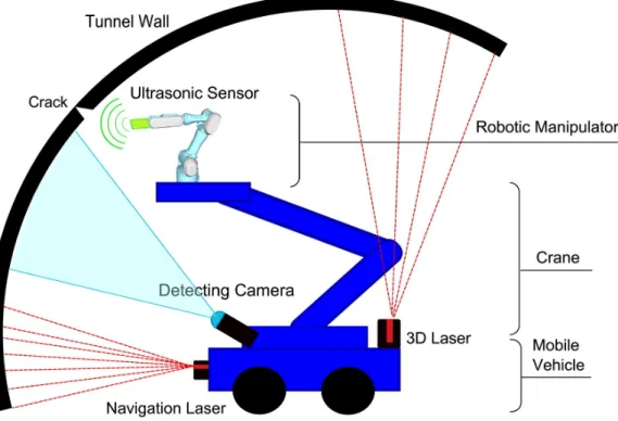
ROBO-SPECT (ROBOtic System with Intelligent Vision and Control for Tunnel Structural inSPECTion and Evaluation) (Montero et al., 2017), (Loupos et al.,
2014), was an EU funded project running from 2013 to 2016. Here, an autonomous vehicle moves along a road tunnel, using a crane to support a manipulator arm with several sensors attached. It uses a range sensor to detect structural deformation, a digital camera to detect cracks, and two RGBD cameras to acquire point cloud data for offline 3D reconstruction of the detected defects.
Figure 3: ROBINSPECT robot diagram (Montero et al.,2017).
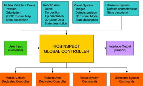
The robot navigates the tunnel using visual marks detected by two laser scan-ners and a digital camera, maintaining a constant distance to the wall. With the digital camera on the arm, the system records its position in space and, if needed, approaches the wall and scans the affected region with the RGBD setup. After this detailed inspection, the system goes back to the earlier pose and resumes the movement along the tunnel. To operate all the systems together, a global controller has been developed with the architecture depicted in Fig.4.
2.2 rail-based duct inspections
Figure 4: Global Controller Architecture used in the ROBINSPECT project (Montero et al.,2017).
The project aimed for tunnel inspection in normal traffic conditions, and the reliability of the system was shown in real life situations. This solution, however, involves a large set of complex subsystems, increasing its size. As such, its use in ducts and manholes is not feasible.
2.2 r a i l - b a s e d d u c t i n s p e c t i o n s
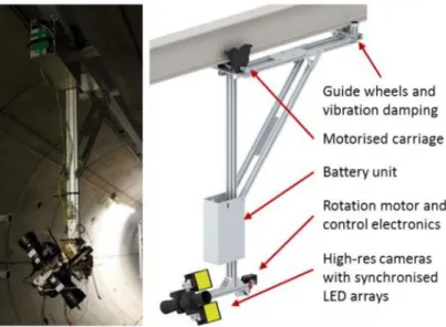
With the increased use of underground ducts for the installation of high voltage power cables (Stent et al.,2015), more frequent inspections will be needed to ensure the integrity of both ducts and cables. In this project, a monorail setting is used to guide an inspection robot carrying digital cameras for later reconstruction of the tunnel’s inner geometry 3D model.
Figure 5: Tunnel reconstruction prototype (Stent et al.,2015).
With two digital cameras placed as shown in Fig. 5, each one with a field of view slightly higher than 180º, an image of a complete section of the tunnel is captured. To get better quality images, the movement is stopped and a set of lenses with polarizing filters (to improve images in wet areas) is used to obtain very accurate images allowing the detection of cracks as thin as 0,3 mm (Fig.6).
Figure 6: Detection and evolution of a crack between sample pictures (Stent et al.,2015).
Captured images are later superimposed to create a point cloud representing the tunnel. The system can also detect the evolution of the size of the cracks size between samples.
For the system to operate with this degree of precision, the duct must be equipped with a rail and supporting structure, rendering the solution expensive. However, having the supporting structure deployed, this represents a very fast way to do the inspection and repeat it, when compared with the typical mobile (track-free) robot solution.
2.3 tunnel inspection using an airborne vehicle
2.3 t u n n e l i n s p e c t i o n u s i n g a n a i r b o r n e v e h i c l e
The project demonstrated the possibility of navigating a tunnel with an airborne vehicle as a base for a later implementation of an inspection system (Ozaslan et al.,
2017). The chosen vehicle, named MAV, exhibits a higher ability to move in a 3D space when compared with wheeled or tracked vehicles. According to the system diagram shown in Fig.7, the system uses four cameras and a 3D laser range scanner to obtain the 3D point cloud, as well as surface pictures of the duct walls. Based on the built point cloud, and on the data generated by an IMU, the system uses a local map and range-based pose estimation to locate the robot in that map. The estimation is later adjusted in a 6 DOF frame using an Unscented Kalman Filter (Simon,2006).
Figure 7: System diagram (Ozaslan et al.,2017).
The system is remotely operated through an interface and requires additional commands to define an initial direction. The reported tests were one-directional, so the main control objective for the trajectory was to maintain the alignment of the vehicle with the center of the duct, as shown by the red line in Fig. 8. Further work is to be done to allow the inspection of branched ducts.
Figure 8: Trajectory (red line) and 3D structure created in real time (Ozaslan et al.,2017).
The project demonstrates advances in pose estimation of an aerial robot in a dark, symmetrical, low in distinctive features, challenging environment. Nevertheless, the authors claim an error limited to 5% for their system.
Although still in a testing phase, the use of the MAV looks promising for au-tonomous inspection. However, only the 3D envelope of the duct was recognized, and no real inspection results are reported. The proposed future work, in that project, has to do with the development of image analysis algorithms to build a panoramic image and to automatically identity defects in the structure.
2.4 v i s u a l i n s p e c t i o n o f a r a i lway t u n n e l
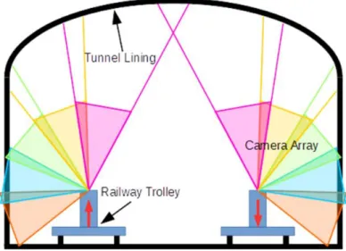
In (David Jenkins et al., 2017), the goal is to develop a low-cost railway tunnel inspection. A set of 5 IP cameras takes overlapping images of the tunnel wall inner surface (see Fig. 9), which are combined afterwards. To avoid shadows, two light sources are directed to the cameras image center.
2.4 visual inspection of a railway tunnel
Figure 9: Position and overlapping of the cameras (David Jenkins et al.,2017).
The choice for IP cameras, is driven by the existence of an on-board computer running the algorithm to compose the images, detect defects, and create a 3D model of the inner structure. This reconstruction maps the pictures onto the 3D mesh to help inspectors understand the contexts and location of the damages. Three steps are as follows in the anomaly feature detection algorithm: first, a comparison is done with an earlier picture (Fig. 10a) with the most likely alignment (Fig.10b) -this alignment is needed, since there is no guarantee that the same spot is covered by a picture taken exactly from the same pose (Fig. 10c); second, once aligned, the images are compared and a mask revealing the differences on the pixels is created (Fig. 10d,) where white pixels represent those differences between inspection runs; in the third, and final step, the mask is applied to the most recent picture showing the perceived changes in red (Fig. 10e).
The detection is not perfect, since a number of false positive results can be observed in the used mask (Fig. 10d) which can be explained from light intensity variation or misalignment from the images.
The system’s travel speed is directly associated to the cameras framerate, and the authors call it a “walking speed”. One can assume that the trolley needs to be pushed by hand, and to capture the other half of the tunnel, either another trolley equipped with their system is needed, or the system must be moved to the other rail manually.
a: Previous image. b: Recent image.
c: Aligned image. d: Mask.
e: Application of the mask to the recent aligned image.
Figure 10: Defect detection process example (David Jenkins et al.,2017).
2.5 i b a k ’ s c o m m e rc i a l a p p l i c at i o n f o r m a n h o l e i n s p e c t i o n "
The "PANORAMO SI 3D Optical Manhole Scanner"1 is a proprietary technology from IBAK allowing the 360º visualization of a manhole in real time. It uses two
2.6 ipek’s manhole inspection system
digital cameras to do the scanning in seconds. Along with the images, a 3D point cloud is also generated so that the integrity of the structure is verified. (Fig. 11).
Figure 11: 3D model of a manhole in the PANORAMO system (IBAK).1
The equipment, however, cannot automatically identify defects and the data must always be analyzed by a qualified person. Nevertheless, it reduces the inspection time spent on site and the risks for the inspectors. The lengthy and thorough analysis is still needed but can be done offline.
2.6 i p e k ’ s m a n h o l e i n s p e c t i o n s y s t e m
The "QuickView" system, from iPEK2, is limited to real time visualization of the images captured by the camera introduced in the manhole. With this camera, it is possible to obtain high zoom level images, which also allows looking into the ducts attached to the manhole, to some extent. It is the cheapest solution, does not reduce the time on site, but still minimizes the risk and comfort problems to the inspector.
3
D E V E L O P M E N T
This chapter presents the reasoning behind the equipment chosen. This includes the systems characteristics, like their resolution and the purpose for what they were built. Since they were not specifically built for manhole inspection, calibrations had to be done to make sure the results obtained would comply with what is expected. This includes the construction of point clouds, shown in Chapter4, as these require the capture system to be properly calibrated, so the model created appears as it is in the real world. If this fails, the model won’t be coherent and, therefore, it won’t have the structure required to be able to conduct an inspection, as if the inspector would have in the real local place. To accommodate each point cloud created, there is the need to use a reference. With the need of also being able to conduct a capture, inside the manhole, using a robot manipulator gave the world reference and the necessary motions. This concept can be seen in Fig. 12.
During the development of this project, extra work was put, to make sure all these systems would synchronize with each other. This work is described in the Appendix, as it does not fit in the computer vision focus of the main objective of this report.
This chapter starts with an explanation of the RGBD camera and the laser point profile sensor chosen. It will continue with their respective calibrations. Such cali-brations include the selection of parameters for capture, as well as the calculus of transformations, to accommodate both point clouds in the same world reference.
3.1 c h o o s i n g t h e rg b d c a m e r a
When this project started, Intel had recently released new RGBD sensors, the D400 family (Keselman et al., 2017). Previous work done in our laboratory (Reis,2018) proved that the goal of providing a 3D model of a manhole for inspection purposes could work, although at that time the error obtained was still large. This new
3.1 choosing the rgbd camera
Table 1: RGB sensor specifications for the Intel Realsense R200, D415 and D435.
Specifications R200 D415 D435 Max. Resolution 1920 x 1080 1920 x 1080 1920 x 1080 Aspect Ratio 16:9 16:9 16:9 Horizontal FOV 70°+/-2° 69.4°+/-3° 69.4°+/-3° Vertical FOV 43°+/-2° 42.5°+/-3° 42.5°+/-3° Diagonal FOV 77°+/-2° 77°+/-3° 77°+/-3°
Table 2: Depth sensor specifications for the Intel Realsense R200, D415 and D435.
Specifications R200 D415 D435 Max. Resolution 640 x 480 1280 x 720 1280 x 720 Aspect Ratio 4:3 16:9 16:9 Horizontal FOV 59°+/-5° 65°+/-2° 87°+/-3° Vertical FOV 46°+/-5° 40°+/-1° 58°+/-1° Diagonal FOV 70°+/-4.5° 72°+/-2° 95°+/-3° Min. Distance 0.5 [m] 0.3 [m] 0.1 [m]
When comparing the R200 with the new D4 family of sensors in their RGB sensor (Table3), there is not much difference or significant evolution between the different series, however, in the case of the depth sensor, it shows a big improvement (see Table2). From the R200 to the D400 series, the depth sensor resolution increased 3 times, with a wider aspect ratio. The field of view also increased by a relevant difference between the D415 and the D435. With a wider FOV, less captures are required for the same area coverage. This, however, is not, in practice, useful, as the RGB sensor’s FOV of the D435 is lower than its depth sensor, rendering the extra image size capture useless, if one wants to capture depth information with texture. As mentioned before, the color reproduction can be a valued ally for the inspection. The minimum distance for capture is another interesting point to take care of in choosing a camera. Previously, with the R200, when constructing the system to accommodate the camera inside the manhole, there was the need to add
was chosen not just because of the 10 cm minimum distance required to the closest object, but also because of its better performance in low light as well (Carfagni et al.,2019). Later on, additional tests were performed with an Intel D415, namely, a small comparison between it and the D435 with the same light conditions, and same camera settings, and at 40 cm of the same scene. In Fig. 13, it can be seen that the D415, even if advertised with a minimum distance to the closest object to perform a distance measure of 30 cm, could not scan the environment. Concluding, comparing the two options, the D415 and the D435, the D435 is the right choice since, inside the manhole, the cameras are at close range to the wall.
3.2 l a s e r p o i n t p ro f i l e s e n s o r
In this project we used the Gocator 20401. This is an industrial-grade laser point profile sensor, used in this project, to generate a ground truth to the 3D model of the manhole inner structure, so as to be used to evaluate the RGBD camera performance. The Gocator 2040 precision is, at the worst case, of 0.049 mm.
Figure 14: Gocator 2040 in its 3D printed support.
1 https://www.stemmer-imaging.com/media/uploads/websites/documents/products/systems/LMI/en-LMI-Gocator-2000-SYLMI1-201410.pdf
3.2 laser point profile sensor
a: D415 depth scene.
b: D435 depth scene.
Figure 13: Comparison between the Intel D415 and D435 cameras in the same scenario. The area inside the red border was at a distance of about 40 cm.
Although this specific model is deprecated, its resolution and precision is more than enough for the overall objective. Since the typical manhole inspection is run with human vision, its safe to assume that the Gocator 2040 can perform a higher visual accuracy scan than the former.
3.3 i n d u s t r i a l ro b o t i c a r m
Unlike the previous work (Reis,2018), no specific mechanical structure was designed for the motion acquisition system. Instead, a robotic arm was used, namely, the KUKA iiwa 7 R8002 (Fig. 15), so has to obtain accurate models. This models will serve as a reference for future implementations with a mechanical structure, developed specifically for this purpose (with lower cost of implementation).
Figure 15: Kuka iiwa 7 R800.
The robot maximum reach is 0.8 m, and with the low mobility inside the man-hole, it cannot retract enough to provide a full inside capture of the manhole. The results obtained contain a small portion of the full manhole. A set of trajectories and targets was specified for the motion acquisition with the robot, using mostly RoboDK3. RobotDK proved helpful in the simulation of collision free trajectories, 2 https://www.kuka.com/en-gb/products/robotics-systems/industrial-robots/lbr-iiwa
3.3 industrial robotic arm
given the tight robot working space. Using a model of the same dimensions as the existing manhole in the lab, it was easy to obtain all the targets required for both the RGBD camera and the Gocator sensor, as compared it to having to teach sev-eral targets manually, avoiding the time wasted of having to recreate a lightweight replica and/or placing the robotic arm inside the manhole just for collision testing. For all the movements inside the manhole, the targets used were based in the joint’s angles, and not cartesian coordinates, avoiding the possible jerk movement associ-ated to letting the robot move to the next target according to its path calculation, and making sure it keeps the wanted orientation. These motions can be briefly seen in Appendix A.2.
To couple the sensors to the flange, two accessories were 3D printed. The first one can be seen in Fig. 16, for the RGBD camera. It also shows a sharp tool used to capture certain points in robot coordinates. The second tool created was for the Gocator 2040, seen attached to its back in Fig. 14.
To be able to reduce vibration, and avoiding a shift in the robot position, gutters were used and screwed in with two M6 bolts on the entrance of the manhole at the base of the robot. So, when capturing data from inside the manhole, the KUKA robot was operated in an inverted position.
Given that the KUKA iiwa is a collaborative robot, its safety conditions were programmed so that the robot would stop upon contact with the inner manhole walls, in order to improve the safety of the operation.
3.4 c a l i b r at i o n o f t h e rg b d c a m e r a
The new Intel RGBD sensor series, D400, uses the new librealsense SDK 2.04. For this new SDK, the cameras can be used with different user selectable presets, in terms of camera parameters. These presets include various parameters that change how the sensor generates depth points. They are namedDefault, Density, Medium Density and High Accuracy5.
3.4.1 Choosing the right preset
Default is the preset that comes selected as default in the camera. Density has the camera parameters tuned in order to capture the most points. Medium Density tries to balance between having as many depth points in the screen and having a high degree of certainty in their depth values.High Accuracy only provides depth points that have a high degree of confidence. These presets were obtained through machine learning algorithms6, so the purpose here is to present the analysis of their output, and not to present additional tuning to the various settings that were already tuned. There was no post-processing applied to the obtained data in the sensor or the Realsense SDK, in order to work with the raw point cloud (for 3D scanning applications, post-processing operations such as hole-filling are not advisable (Grunnet-Jepsen and Tong,2018)). All frames were captured at the maximum resolution of 1280x720, for both color and depth channels, in order to obtain a denser point cloud.
To evaluate the precision of the sensor, 50 frames were obtained for each preset, with the sensor in a fixed position facing the inner wall of the manhole, about 40 4 https://github.com/IntelRealSense/librealsense
5 https://github.com/IntelRealSense/librealsense/wiki/D400-Series-Visual-Presets
6 https://www.intel.com/content/dam/support/us/en/documents/emerging-technologies/ intel-realsense-technology/BKMs_Tuning_RealSense_D4xx_Cam.pdf
3.4 calibration of the rgbd camera
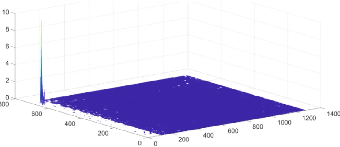
Figure 17: Standard deviation of each cell from the 50 samples, using the Density preset (in meters).
cm away from it. Considering that each acquisition frame is a matrix with depth values in each of the matrix cell positions, the standard deviation can be computed over the set of frames for each cell, resulting in a plot shown in Fig. 17 (for all the 50 frames with Density preset). The optimal result would be a flat plane, but there are outliers with up to 9 m of deviation, much larger than the limits of the manhole. These outliers can be due to the use of artificial light inside the lab, but they mostly appear due to errors in calculating the disparity between the sensor infrared images, likely due to the homogeneous texture of the manhole.
The high standard deviation values arise from readings with large offsets when compared to the expected reading. Given the nature of the problem at hand, there should not be variations in the meters range, in fact, measured distances should be relatively limited. As such, a simple outlier detection was introduced in the depth capture, with values outside the range [0, 50] cm being discarded as invalid ones. This is a filter one can also apply when acquiring data to build the manhole model (recall that the manhole has a 40 cm radius and that the camera was placed in the middle of the manhole, thus allowing for 25% sensor error) - this method was denoted selective standard deviation. Given the computed standard deviation for each pixel across all the acquired frames, the standard deviation and the maximum standard deviation of these values were also computed, in order to understand how precision changes across all the sensor area. The tests where then conducted using this selective standard deviation, with and without the outliers. To see how relevant the outliers were over the selective standard deviation, there was another filter applied in the calculation of the standard deviation. This filter aims at decreasing
0.1888 0.1898 0.1908 0.1918 0.1928 0.1938 0.1948 0.1958 0. 01 0. 04 0. 07 0. 10 0. 13 0. 16 0. 19 0. 22 0. 25 0. 28 0. 31 0. 34 0. 37 0. 40 0. 43 0. 46 0. 49 0. 52 0. 55 0. 58 0. 61 0. 64 0. 67 0. 70 0. 73 0. 76 0. 79 0. 82 0. 85 0. 88 0. 91 0. 94 0. 97 1. 00 St an da rd D ev ia tio n [m m ]
Percentage of the maximum non-valid values present in depth used in the standard deviation[%]
With Outliers
Without Outliers
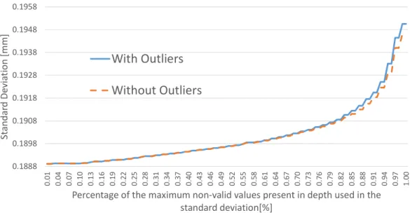
Figure 18: Standard deviation when using theHigh Accuracy preset.
has high confidence. As it can be seen in Fig.18, when the outliers are removed, it does not produce significant changes, with a difference of 0.0044 mm when using all of the data between both situations.
In Fig. 19, which shows the maximum deviation across the entire frame set, including all the data leads to higher differences between both situations (with and without outliers), up to 32 mm. The maximum depth value obtained in this preset was about 1.4 m.
In this experiment, the percentage of points that were not obtained from the sensor and the amount of outliers removed, denoted here as invalid points, were about 22.1%.
The High Accuracy preset, as the name and description indicates, should be the best option, however, the same tests were applied to the other presets. The following figures, 20, 21, 22, 23, 24 and 25, are hard to interpret on paper, due to the discrepancy in values, but can still show how big of a difference and error they can produce from the existing outliers that are generated. At the end of this section, there will be an comparison that should highlight this (Figs.26 and 27).
As shown in Fig. 20, the Default preset shows low precision as it varies signif-icantly between each frame. With the outliers removed, the invalid points were about 14.6% of all points. With this data filtered, it shows a big improvement over the original result, with around 0.186 mm of deviation.
3.4 calibration of the rgbd camera 0.9 1.4 1.9 2.4 2.9 3.4 3.9 4.4 4.9 5.4 5.9 0. 01 0. 04 0. 07 0. 10 0. 13 0. 16 0. 19 0. 22 0. 25 0. 28 0. 31 0. 34 0. 37 0. 40 0. 43 0. 46 0. 49 0. 52 0. 55 0. 58 0. 61 0. 64 0. 67 0. 70 0. 73 0. 76 0. 79 0. 82 0. 85 0. 88 0. 91 0. 94 0. 97 1. 00 M ax im um S ta nd ar d D ev ia tio n [m m ]
Percentage of the maximum non-valid values present in depth used in the standard deviation[%]
With Outliers
Without Outliers
Figure 19: Maximum standard deviation when using theHigh Accuracy preset.
0 0.005 0.01 0.015 0.02 0.025 0.03 0.035 0. 01 0. 04 0. 07 0.1 0. 13 0. 16 0. 19 0. 22 0. 25 0. 28 0. 31 0. 34 0. 37 0.4 0. 43 0. 46 0. 49 0. 52 0. 55 0. 58 0. 61 0. 64 0. 67 0.7 0. 73 0. 76 0. 79 0. 82 0. 85 0. 88 0. 91 0. 94 0. 97 1 St an da rd D ev ia tio n [m ]
Percentage of the maximum non valid values present in depth used in the standard deviation[%]
With Outliers
Without Outliers
0 1 2 3 4 5 6 7 8 9 10 0. 01 0. 04 0. 07 0.1 0. 13 0. 16 0. 19 0. 22 0. 25 0. 28 0. 31 0. 34 0. 37 0.4 0. 43 0. 46 0. 49 0. 52 0. 55 0. 58 0. 61 0. 64 0. 67 0.7 0. 73 0. 76 0. 79 0. 82 0. 85 0. 88 0. 91 0. 94 0. 97 1 M ax iu m S ta nd ar d De vi at io n [m ]
Percentage of the maximum non valid values present in depth used in the standard deviation[%]
With Outliers
Without Outliers
Figure 21: Maximum standard deviation when using theDefault preset.
Its maximum standard deviation (see Fig.21), also had a big improvement, since 10% of the points acquired were outliers with up to 9 m of deviation. Without the outliers, the maximum obtained was about 3 mm.
The Density preset aims to provide a high density point cloud, even if less ac-curate. This leads to an increase in outliers but, in terms of precision, if one only chooses to use points that are valid in at least 20% of all frames, for the standard deviation calculus (Fig.22), the computed values approach that of the filtered one. It is also worth noticing that 11.9% of the total points were outliers, and that the maximum outliers had a lower value than in theDefault preset.
The same happens with the maximum standard deviation, however, as shown in Fig.23, it is seen that it can lead to less precise measures than theDefault preset, with 9.6 m.
The Medium Density preset tries to provide for a highly dense point cloud, but without compromising the accuracy. As shown in Fig. 24, there is a big deviation that can be seen when all the points are used. However, when a minimum of 90% of points with valid values across all frames are used for the standard deviation, it gets close to the filtered sample, with around 0.2 mm of deviation.
The same happens at the maximum deviation value, as shown in Fig. 25, but it does not yield the big deviations from theDefault and Density presets. Only about 10.9% of all points were classified as outliers.
The purpose of the comparison described above was to select a configuration that yields more precise depth values, with less outliers, particularly in a manhole
3.4 calibration of the rgbd camera 0 0.005 0.01 0.015 0.02 0.025 0.03 0.035 0. 01 0. 04 0. 07 0.1 0. 13 0. 16 0. 19 0. 22 0. 25 0. 28 0. 31 0. 34 0. 37 0.4 0. 43 0. 46 0. 49 0. 52 0. 55 0. 58 0. 61 0. 64 0. 67 0.7 0. 73 0. 76 0. 79 0. 82 0. 85 0. 88 0. 91 0. 94 0. 97 1 St an da rd D ev ia tio n [m ]
Percentage of the maximum non valid values present in depth used in the standard deviation[%]
With Outliers
Without Outliers
Figure 22: Standard deviation when using theDefault preset.
0 1 2 3 4 5 6 7 8 9 10 0. 01 0. 04 0. 07 0.1 0. 13 0. 16 0. 19 0. 22 0. 25 0. 28 0. 31 0. 34 0. 37 0.4 0. 43 0. 46 0. 49 0. 52 0. 55 0. 58 0. 61 0. 64 0. 67 0.7 0. 73 0. 76 0. 79 0. 82 0. 85 0. 88 0. 91 0. 94 0. 97 1 M ax im um S ta nd ar d D ev ia tio n [m ]
Percentage of the maximum non valid values present in depth used in the standard deviation[%]
With Outliers
Without Outliers
0 0.2 0.4 0.6 0.8 1 1.2 1.4 1.6 1.8 0. 01 0. 04 0. 07 0.1 0. 13 0. 16 0. 19 0. 22 0. 25 0. 28 0. 31 0. 34 0. 37 0.4 0. 43 0. 46 0. 49 0. 52 0. 55 0. 58 0. 61 0. 64 0. 67 0.7 0. 73 0. 76 0. 79 0. 82 0. 85 0. 88 0. 91 0. 94 0. 97 1 St an da rd D ev ia tio n [m m ]
Percentage of the maximum non valid values present in depth used in the standard deviation[%]
With Outliers
Without Outliers
Figure 24: Standard deviation when using theMedium Density preset.
0 0.1 0.2 0.3 0.4 0.5 0.6 0. 01 0. 04 0. 07 0.1 0. 13 0. 16 0. 19 0. 22 0. 25 0. 28 0. 31 0. 34 0. 37 0.4 0. 43 0. 46 0. 49 0. 52 0. 55 0. 58 0. 61 0. 64 0. 67 0.7 0. 73 0. 76 0. 79 0. 82 0. 85 0. 88 0. 91 0. 94 0. 97 1 M ax im um S ta nd ar d De vi at io n [m ]
Percentage of the maximum non valid values present in depth used in the standard deviation[%]
With Outliers
Without Outliers
3.4 calibration of the rgbd camera
inspection scenario. Figure 26a to26c allows for a direct comparison between the various presets. In Figure26a clearly bothDensity and High Accuracy presets give the best results when no outlier is removed. In Figure26c, it can be seen that the High Accuracy preset has less deviation than the Medium Density preset. Even if it looks like the High Accuracy preset yields a static deviation, it still shows growth, as seen in Figure18. When using 95% of the valid values for the deviation calculus, the Medium Density preset gets closer to the High Accuracy one, but still has a difference of 0.02 mm. In Figure 26b, with the outliers removed, both Default and Medium Density presets lead to less deviation, with very similar results, yielding a minimum deviation of 0.18 mm.
Comparing the maximum standard deviation, Figure 27a to Figure 27c, it is clear that the High Accuracy preset provides the lowest deviation, followed by the Medium Density preset, as shown in Figure27c. As it happened with the standard deviation results, even when choosing 95% of valid values for the calculus, using theHigh Accuracy preset still performs better by about 13 mm. On the other hand, the Default and Density presets can lead to much less precise results, as shown in Figure 27a.
When comparing theHigh Accuracy and Medium Density presets, one also needs to check the amount of depth values that the camera outputs, namely the number of points that were considered valid. The Medium Density preset got the lowest number of outliers with 10.9%, while the High Accuracy preset got 22.1%. Closely evaluating these outliers it is seen that, in the High Accuracy preset, most had depth values of 0 (considered as invalid points), with only 240 points across the 50 images being points with depth value above 50 cm. With the Medium Density preset, the outliers were about 12249 points.
Figure26c and Figure27c also show that, when considering 100% of the acquired points, the Medium Density preset has points that variate more than the double of the High Accuracy preset, which means it is prone to provide higher differences between samples, even in a static scenario. One can perform multiple acquisitions, even from different points of view, in order to produce a more dense point cloud, while retaining the precision of this preset, even if it means some increase in the overall acquisition time.
0 0.005 0.01 0.015 0.02 0.025 0.03 0.035 0. 01 0. 04 0. 07 0. 10 0. 13 0. 16 0. 19 0. 22 0. 25 0. 28 0. 31 0. 34 0. 37 0. 40 0. 43 0. 46 0. 49 0. 52 0. 55 0. 58 0. 61 0. 64 0. 67 0. 70 0. 73 0. 76 0. 79 0. 82 0. 85 0. 88 0. 91 0. 94 0. 97 1. 00 St an da rd D ev ia tio n [m ]
Percentage of the maximum non-valid values present in depth used in the standard deviation[%]
High Accuracy Default Density
Medium Density
a: Standard deviation comparison between all presets.
0.000175 0.00018 0.000185 0.00019 0.000195 0.0002 0.000205 0. 01 0. 04 0. 07 0. 10 0. 13 0. 16 0. 19 0. 22 0. 25 0. 28 0. 31 0. 34 0. 37 0. 40 0. 43 0. 46 0. 49 0. 52 0. 55 0. 58 0. 61 0. 64 0. 67 0. 70 0. 73 0. 76 0. 79 0. 82 0. 85 0. 88 0. 91 0. 94 0. 97 1. 00 St an da rd D ev ia tio n [m ]
Percentage of the maximum non-valid values present in depth used in the standard deviation[%]
High Accuracy Default Density
Medium Density
b: Standard deviation comparison between all presets without outliers.
0 0.2 0.4 0.6 0.8 1 1.2 1.4 1.6 1.8 0. 01 0. 04 0. 07 0. 10 0. 13 0. 16 0. 19 0. 22 0. 25 0. 28 0. 31 0. 34 0. 37 0. 40 0. 43 0. 46 0. 49 0. 52 0. 55 0. 58 0. 61 0. 64 0. 67 0. 70 0. 73 0. 76 0. 79 0. 82 0. 85 0. 88 0. 91 0. 94 0. 97 1. 00 St an da rd D ev ia tio n [m m ]
Percentage of the maximum non-valid values present in depth used in the standard deviation[%]
High Accuracy Medium Density
c: Standard deviation comparison between High Accuracy and Medium Density preset.
3.4 calibration of the rgbd camera 0 1 2 3 4 5 6 7 8 9 10 0. 01 0. 04 0. 07 0. 10 0. 13 0. 16 0. 19 0. 22 0. 25 0. 28 0. 31 0. 34 0. 37 0. 40 0. 43 0. 46 0. 49 0. 52 0. 55 0. 58 0. 61 0. 64 0. 67 0. 70 0. 73 0. 76 0. 79 0. 82 0. 85 0. 88 0. 91 0. 94 0. 97 1. 00 M ax im um S ta nd ar d De vi at io n [m ]
Percentage of the maximum non-valid values present in depth used in the standard deviation[%]
High Accuracy Default Density
Medium Density
a: Maximum standard deviation comparison between all presets.
0 0.002 0.004 0.006 0.008 0.01 0. 01 0. 04 0. 07 0. 10 0. 13 0. 16 0. 19 0. 22 0. 25 0. 28 0. 31 0. 34 0. 37 0. 40 0. 43 0. 46 0. 49 0. 52 0. 55 0. 58 0. 61 0. 64 0. 67 0. 70 0. 73 0. 76 0. 79 0. 82 0. 85 0. 88 0. 91 0. 94 0. 97 1. 00 M ax im um S ta nd ar d De vi at io n [m ]
Percentage of the maximum non-valid values present in depth used in the standard deviation[%]
High Accuracy Default Density
Medium Density
b: Maximum standard deviation comparison between all presets without outliers. 0 0.1 0.2 0.3 0.4 0.5 0.6 0. 01 0. 04 0. 07 0. 10 0. 13 0. 16 0. 19 0. 22 0. 25 0. 28 0. 31 0. 34 0. 37 0. 40 0. 43 0. 46 0. 49 0. 52 0. 55 0. 58 0. 61 0. 64 0. 67 0. 70 0. 73 0. 76 0. 79 0. 82 0. 85 0. 88 0. 91 0. 94 0. 97 1. 00 M ax im um S ta nd ar d D ev ia tio n [m ]
Percentage of the maximum non-valid values present in depth used in the standard deviation[%]
High Accuracy Medium Density
240 33724 22132 12249 0 5000 10000 15000 20000 25000 30000 35000 40000 N um be r o f O ut lie rs Accuracy Default Density Medium
a: Total of outliers discarded between all presets.
10199777 6701276 5496168 5044318 0 2000000 4000000 6000000 8000000 10000000 12000000 N um be r o f 0 's Accuracy Default Density Medium
b: Total of points with no value discarded between all presets.
22.13545356 14.61595486 11.97550564 10.97345269 0 5 10 15 20 25 Pe rc en ta ge o f a ll di sc ar te d pi xe ls a cr os s a ll im ag es [% ] Accuracy Default Density Medium
3.4 calibration of the rgbd camera
Figure 29: Draft of the hand to eye calibration made (Ali et al.,2019).
3.4.2 Extrinsic camera parameters
Using the 3D printed support for the RGBD camera, there was the need to dis-cover the transformation required to transform the points obtained in camera coor-dinates to robot coorcoor-dinates. For this, 4 captures were made from different angles and positions of a checkerboard picture, while saving the flange position in robot coordinates and associating it with the respective picture. A visual representation of this method can be seen in Fig. 29.
Knowing that the left infrared sensor of the RGBD camera was the origin of its reference, a camera calibration using a chessboard pattern was made (Ali et al.,
2019). The extrinsic parameters were obtainable through the librealsense SDK and were as follows (transformation in homogeneous coordinates):
K = 642.701 0 644.221 0 642.701 350.991 0 0 1
Having obtained the extrinsic parameters, which shows the position of the camera in the chess pattern coordinates (lets call it cam Pchess), the next step is to know
obtained. Multiplying this last transformation with the position of the camera in chess coordinates, results in the camera position in robot coordinates (camProbot):
camProbot =chessTrobot∗camPchess
In the last step, one uses the flange position in robot coordinates (f lange P robot) for the respective image. Since the goal is to obtain the transformation between the camera and flange (camTf lange), then it results as follows:
camProbot =camTf lange∗f langeP
robot <=>
<=>camTf lange = (f langeP
robot)−1∗camProbot
With the transformation between camera and flange obtained, the stitching of the pointclouds can be obtained through the multiplication of each point in the pointcloud (Pointcam) with the transformation of the camera coordinates to the robot coordinates (cam Trobot), depending on the position of the flange in robot coordinates of the respective picture. This calculation when applied to all points, results in a pointcloud in robot coordinates:
P ointrobot = (camTf lange∗f langeProbot) ∗ P ointcam
3.5 c a l i b r at i o n o f t h e l a s e r p o i n t p ro f i l e s e n s o r
The calibration of the laser point profile sensor first needs an integration with the robot manipulator. This integration is to make sure that, for every Gocator’s capture, the robot’s position is the one that corresponds at the time of the Gocator’s capture. Once this is finished, then a calibration to determine the transformation from Gocator’s coordinates to robot coordinates, can be calculated, using the same method previously used with the RGBD camera.
This section will start describing the process made to accomplish a communication between KUKA and Gocator, for the capture to position synchronization. It will then be followed with the process made to calculate the transformation required to transform the Gocator’s points into robot points, resulting in a point cloud that can be seen in Chapter4.
3.5 calibration of the laser point profile sensor
3.5.1 Communication between KUKA and Gocator
The Gocator 2040 is capable of building 3D models of objects in motion, if it has access to encoder data from that motion. The Gocator itself is usually still, and the object to be scanned needs to pass through the Gocator’s own laser beam. This is typically used with a conveyer in mind, where the Gocator, staying still, can track the distance that the object has moved with signal inputs from the conveyer’s encoder. With the use of a robotic arm, the motion information can be obtained by knowing the Gocator’s position at the time of the capture.
To use and combine both the Gocator and KUKA, there was the need to make sure both communicate motion information. Since the KUKA’s controller is relatively closed, in implementing external programming libraries, like the Gocator libraries, an external computer was used to receive the communication from both systems. Using the Fast Research Interface7 communication from KUKA, allowed for a fast communication between computer and KUKA, being able to receive KUKA’s poses every 1 ms. Computer Gocator 2040 Kuka iiwa R7 800 TCP/IP FRI
Figure 30: Initial diagram of communications between Gocator and KUKA.
A drawback of using the FRI, is that, the robot kinematics have to be calculated externaly, since, it only returns the value of each joint. It was then used a TCP/IP communication to receive the pose in XYZ coordinates from KUKA, even if it meant a lower packet transmission frequency. Using Gocator’s and Kuka’s timestamps, there was the need to synchronize their messages. This required that both clocks be synchronized. However, the Gocator does not support a NTP server, as KUKA does,
first capture received. The following messages, subtracted with the initial capture, would give the passed time in microseconds. After all messages were received, a linear interpolation was used according to the timestamps in the computer’s clock, to try to reduce any error to the upcoming calibration. With this communication system built, tests started to show a problem. The Gocator 2040 clock, was having a delay in the communication over time. This clock drift could be easily seen, by performing a simple up and down movement, while attached to KUKA, as shown in Fig. 31. By normalizing the distance value from Gocator, and the Z value of KUKA, it was possible to synchronize them so they could be visualized together, as for example, the highest distance registered from Gocator would be the highest Z value from KUKA.
0 0.5 1 1.5 2 2.5 Time [ms] 105 0 0.1 0.2 0.3 0.4 0.5 0.6 0.7 0.8 0.9 1 Gocator Kuka
Figure 31: Delay present from Gocator over time.
At around 50 seconds of scanning, Gocator was having a delay of almost a full second. At this time, the Gocator was always set up to capture with its highest frequency of 301 Hz. This meant that the time between captures was around 3.32 ms. Instead of using the Gocator’s time messages in computer’s time, the 3.32 ms was simply added consecutively after the first message for every other one. This
3.5 calibration of the laser point profile sensor
in long scan periods, still added to the error. As such, a different synchronization method was implemented, by using the robot and Gocator’ digital I/O.
With this new synchronization scheme, where KUKA was the master, given that it had higher packets transmission frequency, and Gocator the slave. Now, Kuka controls when a capture is taken, so the number of messages received in the com-puter should be the same between Gocator and Kuka. This however, presented another issue, as the number of signals that KUKA was sending to Gocator were less than what was received in the computer. Using a logic analyser, it was possible to measure the number of signals that KUKA was outputting to fire Gocator’s capture, and after filtering some noise from the hardware built to accommodate the communication (that can be seen in AppendixA.1), the only way to receive the same number of messages was to add a delay between each signal sent to Gocator. According to the Gocator Manual, it is noted that the processing of each frame might take up to 20 ms, however, this was not a problem as previously noted when using its max frequency. It was then assumed that this delay is part of its signal receiving infrastructure. To circumvent this problem, the Gocator started being the master, and since it was not possible to send a digital signal once a capture was finished processing (that feature is not available for this sensor), the signal from Gocator to Kuka, had a delay of 16 [ms] once a capture was started. This delay was selected after multiple tests with different delays, over long periods of time. Anything higher than 16 [ms] showed a minimal improvement with a lower frequency of messages.
The signals flow starts with a signal from KUKA to Gocator, allowing Gocator to start a capture. KUKA waits for the signal, with 16 [ms] of delay, from the Gocator to go low, signaling that the capture was processed. KUKA ends up not sending a digital signal with a certain duty-cycle, it just reacts from the Gocator signals as seen in Fig.32.
Kuka
Gocator
Time
16 [ms]
Wait for Gocator's signal
to go 0
Figure 32: Digital signal communication between Gocator and KUKA.
With the last adjustments, the structure for communication is shown in Fig.
33. Note that, when KUKA’s signal goes low, it does not go at the same time as Gocator’s goes high. This is because, KUKA has a variable delay whenever it checks the signal. The same applies when it needs to detect the descent from Gocator’s signal to low. At best, this delay should be of only 1 ms. With this setup is noted that there is an increased delay between the saved position from KUKA and the corresponding Gocator’s, however this is seen as minimal, and, compared to the original output with the timestamps, there appears no more noticeable delay overtime. Computer Gocator 2040 Kuka iiwa R7 800 TCP/IP TCP/IP Digital Signals
Figure 33: Final diagram of communications between Gocator and KUKA.
Fig.34shows the result of the test previously done in Fig.31with this final setup. When looking at these tests, some holes can be seen as missing the position from KUKA. They can be seen towards the end, in Fig. 31. Since KUKA’s controller is running in an actual Windows machine, the system, even if it prioritizes the execution of the motions, it fails in providing a seamless execution of other tasks. This means, that from time to time, an instruction may take longer to be executed
3.5 calibration of the laser point profile sensor
than expected. In the end, the frequency between each capture is around 50 Hz, 6 times lower than the initial 300 Hz.
1.5621672 1.56216725 1.5621673 1.56216735 1.5621674 1.56216745 1.5621675 1.56216755 Time [ms] 1012 0 0.1 0.2 0.3 0.4 0.5 0.6 0.7 0.8 0.9 1 Gocator Kuka
Figure 34: Delay fixed but KUKA presents interruptions sporadically.
The communication and its flowchart can viewed more in depth in AppendixB.
3.5.2 Calibration with the Gocator
The Gocator calibration approach uses the hand to eye calibration method. There is no reference in the Gocator’s manual as to its origin of reference, so as a starting point, it was defined as the centre point of the laser projector visor’s area. Unlike, the checkerboard pattern used with the RGBD camera previously, a parallelepiped object was used. Initially, several markers in the scene were identified in robot coordinates, like letters carved onto the object, but once the data from the Gocator is reviewed, it is hard to recognize the shapes and identifying the corners, since the
coordinates of its centre with KUKA. This also had an advantage of being a known form and, no matter how different the angle from the scene was, it could always be identified as an ellipse and, therefore, obtain its geometric centre. These holes were also different in size, to help identify which hole is which, and, although it was not implemented, an automatic process of identifying the holes could be developed. After doing four different captures, three with a rotation of an axis and the last one without any rotation, the holes were categorized and identified for each movement manually.
Figure 35: Object with holes for Gocator calibration.
After the holes being identified, an ellipse was fitted to each one, and its geomet-ric centre computed. This gemotgeomet-ric centre, in Gocator’s coordinates, is then asso-ciated with the closest position obtained from KUKA through linear interpolation, between the closest 2 positions relative to the geometric centre obtained, accord-ing to the distance between captures from the centre coordinates. After havaccord-ing all points (8 points for each movement, 32 points in total), in Gocator coordinates, associated with their respective KUKA coordinates, the transformation between Gocator coordinates to KUKA coordinates could be computed. To determine the transformation parameters, the problem was approached as an optimization prob-lem. The variables to obtain were “X”,”Y”,”Z” and its respective rotations, “C”,”B”,
3.5 calibration of the laser point profile sensor
and “A”. Since the rotations are in radians, to make sure the optimizer was giving every variable the same importance, a normalization had to be done. The cost for the function is the square sum of the error between the estimated coordinate of each point and its real robot coordinates. The reason for the square sum instead of the sum is just so that the error sum always adds up.
The results, shown in Fig.36, were not very accurate. The holes should be aligned between movements and belong in the same plane. This was likely due to an error in the measure of each point in robot coordinates, the existent delay from commu-nication, as well as the calculation of the hole’s centre in Gocator’s coordinates.
Figure 36: Calibration with significant error using the first approach. Each color corre-sponds to a different movement.
To minimize this error the approach in the cost function was redone. This time, instead of calculating the difference between the estimated and the real position, the purpose was to make sure the centre of each hole for all movements (M1, M2, M3 and M4), was as close as possible. The function cost for each of the 8 points (for n movements) becomes:
Mmean=
M1+ M2+ M3+ M4 4
Cost = 8 X n=1
Errorn2
By using this cost function in the optimization problem, one obtains better re-sults, since it removes the error of the real manually measured points in robot coordinates, as it can be seen in Fig37.
Figure 37: Calibration using the second approach. Each color corresponds to a different movement.
When scanning a different object, this time with three different movements, the resulting 3D point cloud shows good visual integrity (Fig.38). By closer inspection, in this same scenario, it can be seen, at times, an error of 0.5 mm between different captures as shown in Fig.39.
3.5 calibration of the laser point profile sensor
Figure 38: 3D point cloud from a wood object with Gocator. Each color corresponds to a different movement.
Figure 39: Difference observed of 0.5 [mm] between movements from Gocator’s point cloud. Each color corresponds to a different movement.
The error obtained is below 1 mm precision. Nevertheless, using more diverse trajectories during the calibration would lead even lower errors. This was noted as the quality of the calibration done with 4 trajectories, as opposed to 2, presented better results, even if the optimization solution gave an higher number. This is due to the error being the sum of its square value as well, due to having more points
gocT robot= 1 −0.0018 −0.0023 0.9206 0.0018 1 0.0009 65.502 0.0023 −0.0009 1 70.8474 0 0 0 1
4
R E S U LT S A N D C O M PA R I S O N
In this Chapter, both Gocator’s and Intel’s point clouds were obtained from the respective transformations calculated in Chapter 3. There is an analysis for each point cloud properties, including overall visual quality, and structural integrity. In the last section, the final comparison will be drawn, using Gocator’s final point cloud as the ground truth, for the final Intel’s point cloud.
4.1 i n t e l rg b d c a m e r a r e s u lt s
Using the Intel RGBD D435 inside the manhole, 18 captures were taken between each strip, so every consecutive horizontal rotation was of 20 degrees. There were also a total of 3 different full strips of the manhole taken with different heights. When adding every capture together, there was reasonable overlapping, leading to processing overhead when trying to visualize the point cloud. In total, for each strip, only 7 captures were needed and the strips were spaced out at 22 cm from their center of mass. Due to the space restraints inside the manhole, and the robot limitations therein, only a 22 cm height strip was captured. Previously noted, the D435 depth sensor provides a bigger FOV than its RGB sensor, so all of the extra depth points obtained, resulted with no real color. These points appear as a copy of the last obtained color from the texture picture, as seen in Fig.40.
Figure 40: Depth sensor FOV being wider than the RGB sensor provides a dragged color.
Removing the extra points with no color, the color presented is quite alike to that of the manhole. During this test, the only source of light was of an halogen lamp placed at the entrance of the manhole, at about 1 m away from the capture. The manhole itself is built with different cylindrical blocks, and the camera happened to capture the junction of two of these. In the capture it looks like there is a gap of around 2 cm at this junction. Given the used preset only returns depth when there is reasonable confidence, the camera’s angle, when faced at the wall, could potentially obstruct the depth of the gap between the manhole blocks. The manhole does not have its blocks perfectly aligned, since they are not attached to each other, even if not visible from the outside, as seen as in Fig.41, which represents the RGB picture at the same angle of the previous seen point cloud.
4.1 intel rgbd camera results
Figure 41: Picture of inner wall of the manhole.
If there was direct illumination onto the scene of picture, the camera could have obtained additional points indicating a difference in depth in the junction, but, as of now, the point cloud obtained represents what could happen if there was a visible crack in the wall in the same setup. Across the point cloud it can also be noted, that further away from the center of the picture, holes start to appear, even if these do not exist in reality as their size or depth suggest. This could be fixed by using all of the captures taken, since the holes could be overlapped with another capture, by using direct illumination, and is something to be addressed in the future. When stitching all point clouds together, the model obtained is as presented in Fig.42.
Figure 42: 3D manhole model obtained with the Intel D435 camera.
The model obtained, when compared with the result from the previous work (Fig.
43), shows a big improvement in definition and especially in color reproduction, even if it didn’t had a light source projecting on to the scene.
Figure 43: 3D manhole model obtained with the Intel R200 camera (Reis,2018).
When looking at all of the captures, there were noticeable points outside the dimension of the manhole. Although rare, this still happened even if not shown
4.1 intel rgbd camera results
in the pictures, since it is hard to discern a single point from the others. These outliers appeared with distances of several meters. This was even more apparent when trying to build the whole model of the manhole with sharper angles of the scene. For this take, the camera took pictures from a lot more angles, trying to cover the rest of the manhole. The results, after filtering most outliers, can be seen in Fig. 44.
Figure 44: 3D full manhole model obtained with the Intel D435 camera without color.
at 1 m of distance in the case where the camera is at the bottom looking at the entrance on the top of the manhole. There is a big visible missing part from the manhole, partially due to the robot not being able to do a full consecutive 360 degree movement, leaving the camera missing parts of the wall when looking up, most point clouds barely overlapped. This could be fixed by changing some targets of the KUKA’s movement.
4.2 g o c at o r 2 0 4 0 r e s u lt s
The Gocator’s manhole capture had two long captures per strip. Since the KUKA cannot do a consecutive 360 degree movement, especially considering the orienta-tion that Gocator must be in to perform a scan, there was the need to do a 180 degree rotation of the flange between the two long 180 degrees captures. This meant that, in height, KUKA was again, severely constrained to make sure to not touch the walls during this movements. The first and last strip taken, were separated by 20 cm. This does not mean that the capture area was almost as the same as the camera, since the Gocator can only capture around 15 cm of vertical height at the distance of 20 cm from the wall. To be able to make sure the captures were overlapping in order to stitch them, 3 full strips had to be taken, with 10 cm of height separating them. The obtained model obtained is shown in Fig. 45. Recall that, with the Gocator, one can only obtain positional information, not texture.
4.2 gocator 2040 results
Apart from the lack of color, Gocator presents higher definition compared to the D435’s model. It also lacks the sizeable holes that exist in the former’s point cloud. However, as previous noted, the transformation calculated for the Gocator appears to reveal a bigger error in this case. When each capture overlaps, a bigger difference can be noted, as noted in Fig. 46.
Figure 46: Error from the Gocator’s 3D manhole model. Note that the Depth value corre-sponds to the Y axis in this case.
In some parts, particularly at the end from a capture, this difference can reach up to around 2.5 mm. This means that there should be more work put on into cal-ibration, to provide a better ground truth for the upcoming comparison, although, the stitching applied to this point cloud is going to reduce part of this error. Lastly, when looking at the point cloud closely, one can see the interruptions when KUKA had a delay between instructions, as seen by the spacing without points, in multiple areas of the image (see Fig. 47).
Figure 47: Spacing in Gocator’s point cloud from KUKA’s own delays.
4.3 c o m pa r i s o n i n m a n h o l e m o d e l s
Before comparing directly, both point clouds need to be constrained to the same space. As the Intel’s camera point cloud provides higher FOV range, its height was trimmed down to the same range as Gocator’s point cloud output. To directly compare this two point clouds in particular, the height becomes our basis of com-parison. The remaining axis are the ones that are going to be compared. Fitting