Repositório Institucional UFC: Contributions to the two-dimensional guillotine cutting stock problem

(1)

CENTRO DE CIÊNCIAS

DEPARTAMENTO DE ESTATÍSTICA E MATEMÁTICA APLICADA MESTRADO EM MODELAGEM E MÉTODOS QUANTITATIVOS

RONALDO LAGE PESSOA

CONTRIBUTIONS TO THE TWO-DIMENSIONAL GUILLOTINE CUTTING STOCK PROBLEM

(2)

Dissertação apresentada ao Curso de Mestrado em Modelagem e Métodos Quantitativos do Departamento de Estatística e Matemática Aplicada do Centro de Ciências da Universidade Federal do Ceará, como requisito parcial à obtenção do título de mestre em Modelagem e Métodos Quantitativos. Área de Concentração: Otimização e Inteligência Computacional

Orientador: Prof. Dr. Bruno de Athayde Prata

Co-Orientador: Prof. Dr. Carlos Diego Rodrigues

(3)

Dissertação apresentada ao Curso de Mestrado em Modelagem e Métodos Quantitativos do Departamento de Estatística e Matemática Aplicada do Centro de Ciências da Universidade Federal do Ceará, como requisito parcial à obtenção do título de mestre em Modelagem e Métodos Quantitativos. Área de Concentração: Otimização e Inteligência Computacional

Aprovada em:

BANCA EXAMINADORA

Prof. Dr. Bruno de Athayde Prata (Orientador) Universidade Federal do Ceará (UFC)

Prof. Dr. Carlos Diego Rodrigues (Co-Orientador) Universidade Federal do Ceará (UFC)

Prof. Dr. Albert Einstein F. Muritiba Universidade Federal do Ceará (UFC)

Prof. Dr. Reinaldo Morabito

(4)

(5)

Agradeço inicialmente a Deus que, por intermédio de Nossa Senhora, permitiu que o presente trabalho pudesse ser finalizado no prazo e qualidade desejada, mesmo com todas as barreiras pessoais que surgiram durante o seu desenvolvimento.

A minha esposa Larissa, pela paciência, compreensão e o esforço extra nos cuidados do nosso filho, tendo ele nascido durante o desenvolvimento desta pesquisa.

Ao meu filho Miguel, para o qual todo o esforço despendido nesse trabalho foi dedicado.

A CAPES, pelo apoio fornecido através da bolsa de pesquisa, permitindo a dedicação total a esta pesquisa.

(6)

ência.”

(7)

No presente trabalho são apresentadas duas novas variantes do problema de corte guilhotinado bi-dimensional. São propostas formulações matemáticas e métodos de solução para lidar com os problemas apresentados. Primeiramente, é apresentado o problema de corte guilhotinado bi-dimensional de dois-estágios no qual os itens são idênticos, as placas têm tamanhos diferentes e o objetivo é determinar o tamanho ótimo dos itens idênticos. Dois procedimentos de solução são apresentados para resolver o caso no qual a orientação dos itens é fixa e o caso no qual a rotação ortogonal dos itens é permitida. Os dois procedimentos lidam com o problema resolvendo iterativamente um problema da mochila para cada tamanho possível de item e retornando a melhor solução encontrada. Experimentos numéricos são conduzidos para avaliar a escalabilidade das abordagens. Por último, é apresentado o problema de corte bi-dimensional guilhotinado de

k-estágios no qual o custo desetupassociado aos estágios de corte é considerado relevante. Uma

formulação matemática comO(n2pN)variáveis eO(npN)restrições é apresentada, onde,n, p

e ksão o número de itens, placas e estágios, respectivamente. Experimentos computacionais

foram conduzidos em vinte instâncias de pequena escala geradas aleatoriamente para avaliar a qualidade da abordagem.

Palavras-chave: Problemas de corte e empacotamento; Itens idênticos;Setup; Corte em estágios;

(8)

In this work we present two new variants of the two-dimensional guillotine cutting stock problem. We propose mathematical formulations and solution methods to deal with such problems. Firstly, we deal with the two-stage two-dimensional guillotine cutting stock problem in which items are identical, bins are different in size and the objective is to determine the optimal size of the identical items. Two solution procedures are presented to solve the case in which the orientation of the items is fixed and the case in which orthogonal rotation of items is allowed. The two procedures deal with the problem iteratively solving a knapsack problem for each possible item size and returning the best solution found. Numerical experiments are conducted on two- hundred randomly generated instances to evaluate the scalability of the approaches. Lastly, we deal with thek-stage two-dimensional guillotine cutting stock problem in which setup cost associated with

stages of cut are considered relevant. A mathematical programming formulation withO(n2pk) variables andO(npk)constraints is present, in whichn,pandkare the number of items, bins

and stages, respectively. Numerical experiments are conducted on twenty small-scale randomly generated instances to evaluate the quality of the approach.

(9)

Figure 1 – Contributions of the Thesis . . . 14

Figure 2 – Strip pattern example . . . 20

Figure 3 – Solution for instance 4 -K1 . . . 30

Figure 4 – Solution for instance 4 -_K2 . . . 30

Figure 5 – Computational time (non-rotational) . . . 30

Figure 6 – Computational time (rotational) . . . 31

Figure 7 – Computational time x Number of items (M1) . . . 31

Figure 8 – Computational time x Number of items (_K2) . . . 32

Figure 9 – Four-stage cutting pattern . . . 38

Figure 10 – Four-stage cutting procedure . . . 39

Figure 11 – Solution for instance 4 withk=5 and low setup configuration . . . 49

(10)

Table 1 – Computational results (non-rotational) . . . 28

Table 2 – Computational results (rotational) . . . 29

Table 3 – Instances . . . 46

Table 4 – Dummy items . . . 47

Table 5 – Computational results (k=3) . . . 48

Table 6 – Computational results (k=4) . . . 48

(11)

Algorithm 1 – Knapsack procedure 1 . . . 23

Algorithm 2 – Solution procedure_K2 . . . 25

Algorithm 3 – Dominated items elimination procedure . . . 26

(12)

1 INTRODUCTION . . . 12

2 A TWO-DIMENSIONAL GUILLOTINED CUTTING STOCK PRO-BLEM CONSIDERING THE OPTIMAL ITEM SIZE DETERMINA-TION . . . 15

REFERENCES . . . 34

3 AK-STAGE TWO-DIMENSIONAL GUILLOTINE CUTTING STOCK PROBLEM WITH SETUP COSTS . . . 37

REFERENCES . . . 51

4 CONCLUSIONS AND FUTURE WORKS . . . 54

(13)

1 INTRODUCTION

Cutting and Packing Problems (CPP) are a class of combinatorial problems widely studied in the last few decades. Several variants are reported in the revised literature, however, taking into consideration some criteria and constraints, there are several practical characteristics of the problem that have not been addressed.

Two-dimensional cutting problems have the objective of obtaining a set of small objects (items) from a set of large objects (bins). In some practical cases, such as for granite cutting, an additional limitation is imposed regarding the assortment of items known as guillotine cutting. A guillotine cut is defined as an orthogonal edge-to-edge cut applied to an object resulting in two new objects that can be a desired item or a smaller bin to be cut later. A cut stage is a set of parallel guillotine cuts performed on a bin or on the resulting sub-bins from previous stages.

In this work, we present two variants of the two-dimensional guillotine cutting stock problem not addressed in the revised literature so far. Firstly, we deal with the problem of finding the optimal size of the identical items to be obtained from a set of bins of different sizes. Moreover, we deal with a second problem of evaluating the trade-off between material waste associated with the decision regarding cut patterns and setup cost associated with the complexity of cutting patterns used. These problems have a practical relevance as they were identified during technical visits to a local granite industry.

During the visits, several difficulties were highlighted by the budget analyst regarding the cutting planning and customer requirements. According to the analyst, stock pieces are internally produced by cutting granite blocks into rectangular plates and, due to deviation between the dimensions of the blocks, the plates produced are different in size. This heterogeneity of bins is a huge hindrance to the cutting planning considering it is done with the use of spreadsheets.

The company participates in biddings for the supply of materials for the construction of large ventures such as airports and shopping centers, hence the assortment by spreadsheet can take from hours to a couple of days, making the whole process time-consuming and costly.

(14)

in the possible lowest budget. For this case, to guarantee a low production cost, it is preferable that the cuts are performed in a maximum of two stages. The difficulty of the process of finding the optimal item size is increased by the heterogeneity of bins and the large number of item size possibilities.

Furthermore, the analyst reported another issue associated with production cost concerning the cut patterns. According to him, depending on the material cost, one can sacrifice the optimization of the plate area usage if the associated cutting plan is operationally easier to be executed. The complexity of a cut plan is associated with the number of cut stages required to obtain the desired items.

Therefore, we define our first problem as a non-exact two-stage two-dimensional guillotine cutting stock problem in which the objective is to decide the size of the identical items to be obtained from a set of bins of different sizes in order to fulfill a demand at minimum cost. Finally, our second problem is defined as a non-exactk-stage two-dimensional guillotine cutting

stock problem with items and bins of different sizes in which setup cost associated with the use of cut stages is considered.

Figure 1 shows the characteristics of the two problems according to the typology presented by Wäscheret al.(2007). Both problems are assigned as input minimization problems,

which means that the objective is to minimize cost associated with bin usage. On the item size problem we deal with a set of identical items and, on the setup problem, we deal with a strongly heterogeneous set of items. For both problems, the set of bins is also strongly heterogeneous.

(15)

Figure 1 – Contributions of the Thesis

(16)

2 A TWO-DIMENSIONAL GUILLOTINED CUTTING STOCK PROBLEM CONSI-DERING THE OPTIMAL ITEM SIZE DETERMINATION

RESUMO

No presente trabalho é proposta uma nova variante do problema de corte bi-dimensional gui-lhotinado na qual a decisão está associada a escolha das dimensõesh(altura) ew(largura) dos

itens idênticos a serem obtidos a partir de um conjunto de placas heterogêneas com o objetivo de atender uma demanda a custo mínimo. Modelos matemáticos e procedimentos são apre-sentados para solucionar os casos com e sem rotação ortogonal de itens. Os procedimentos lidam com a variante na qual o conjunto de possíveis tipos de itens é finita (discreta), resolvendo iterativamente um modelo matemático para cada tipo de item possível e retornando a melhor solução encontrada. Experimentos computacionais executados em instâncias aleatórias mostram a eficácia da abordagem.

Palavras-chave: Problemas de corte e empacotamento; Itens idênticos; Corte Guilhotinado; Programação matemática, Problema da Mochila.

ABSTRACT

This paper proposes a new variant of the two-dimensional guillotine cutting stock problem in which the decision is associated with the choice of dimensionsh (height) and w (width) of

the identical items to be cut from a set of heterogeneous stock pieces (bins) in order to fulfill a demand at minimum cost. Mathematical models and solution procedures are presented for solving the cases with and without orthogonal rotational of items. The procedures deal with the variant where the set of possible dimensions for the identical items is finite (discrete) by iteratively solving a mathematical model for each possible item type and returning the best solution found. Computational experiments performed on randomly generated instances show the effectiveness of our approach.

(17)

INTRODUCTION

Cutting stock problems appear in several industrial processes where certain materials such as glass, steel, wood or granite are cut to produce smaller items in order to fulfill customer demands. The items may have different shapes such as rectangular, circular or more complex structures. The process of cutting rectangular bins into smaller rectangular items may have technical limitations regarding the equipment used or the material being cut, e.g., some materials such as glass, ceramics and granite may only be cut from edge-to-edge of the material.

The variant proposed in this paper emerged from the granite industry during technical visits to a local manufacture. In this practical case, the bins are different in size and the cut patterns are done manually by the budget analyst. Throughout the visits, the budget analyst highlighted a few difficulties regarding customers requirements, reporting two types of quotation requests. In the first case the customer specifies the sizes and quantities of the items, and, in the second case, the customer specifies the desired total square footage and lets the company decide the size of the identical items.

The budget depends on the average percentage loss, which means that choosing the size of the identical items would allow the possibility of finding a lower budget. In addition, the cuts should preferably be performed in two stages. This premise is based on the need for productivity. Given the variability of sizes of bins and the large number of item size possibilities, this process can become extremely time consuming. Moreover, it is highly unlikely that the analyst will find a good or the best solution as the process is done manually by the use of spreadsheets.

Therefore, we define our problem as a two-stage two-dimensional cutting stock pro-blem with variable bin size in which we decide the dimensions of the identical items. Throughout this paper we will refer to this problem as the Item Size Problem (ISP). The problem under study presents a close relation to the two-dimensional manufacturer’s pallet loading problem, more specifically the guillotine restricted case.

Ram (1992) presents a survey on the pallet loading problem. The survey includes considerations in pallet packing, models and solutions methods. Morabito and Morales (1998), Morabito and Farago (2002), Birginet al.(2005), Pureza and Morabito (2006) and Ribeiro and

Lorena (2007) have addressed the manufacturer’s pallet loading problem.

Wäscheret al.(2007) provide a typology of cutting and packing problems improved

(18)

as an input maximization problem, in which a single pallet is loaded with the maximum number of identical boxes.

The problem under study has a restriction associated with the type of cut known as guillotine cutting. Many authors have addressed the guillotine cutting stock problem, e.g, Gilmore and Gomory (1965), MacLeodet al.(1993), Christofides and Hadjiconstantinou (1995),

Vanderbeck (2001), Alvarez-Valdeset al. (2002), Songet al.(2004), Belov and Scheithauer

(2006), Hifiet al.(2012), Morabito and Pureza (2010), Furini and Malaguti (2013), Cuiet al.

(2014), Lodiet al.(2015), Andradeet al.(2016) and Furiniet al.(2016).

Steudel (1979) presents a heuristic algorithm to generate pallet loading patterns. The problem is defined as a two-dimensional cutting stock problem in which all the small items have the same dimensions and non-guillotine cuts are allowed. Later, Ghandforoush and Daniels (1992) use a rule-based programming language for determining the packing of identical items inside a large objective with the objective of minimizing waste.

Young-Gun and Kang (2001) deal with the two-dimensional pallet problem with the objective of maximizing the number of identical items loaded onto a large rectangle. The authors propose a new heuristic algorithm to find solutions having a 5-block structure when non-guillotine patterns are allowed. Birgin et al. (2005) provide notes on anL-approach for

solving the manufacturer’s pallet loading problem previously studied by Linset al.(2003). Later,

Birginet al.(2010) combine an improved version of the 5-block heuristic with anL-approach

for packing rectangles into larger rectangles andL-shaped pieces.

Alvarez-Valdés et al.(2005) take the advantage of the relation between the pallet

loading problem and the maximum independent set problem to propose a branch-and-cut al-gorithm for the first problem. Later, Pureza and Morabito (2006) perform experiments with a tabu search algorithm for the non-guillotine manufacturer’s pallet loading problem. Birgin and Lobato (2010) propose a mixed integer continuous nonlinear model for the orthogonal packing of identical rectangles within isotropic convex regions, i.e., non-rectangle large objects.

(19)

solution methods are exposed; (iii) in the fourth section, the mathematical models and solution methods are numerically tested and the results are discussed; (iv) at the end, the paper presents some conclusions and recommendations for future research.

MATHEMATICAL FORMULATIONS

Non-rotational ISP formulation

The following model, which we will refer to as_M1, concerns the non-rotational ISP. In this model, we consider the set of possible item types to be limited, i.e, the dimensions of the items are discretized. Due to the identical dimensions of items, the assortment of items can easily meet the guillotine restriction by simply packing the items side by side. In what follows, some notation is introduced for the proposed model.

Sets and indexes

l∈B={1, . . . ,p}: set of bins; i∈I={1, . . . ,n}set of item types. Parameters

Hl: height of binl; Wl: width of binl; cl: cost of binl;

hi: height of item typei; wi: width of item typei; A: area demand;

ail =hiwi

j

Wl wi

k j

Hl hi

k

: useful area of binlwith respect to item typei.

Decision variables

(20)

Objective function Minimize

_∑

l∈B

∑

i∈I

cluil (2.1)

Constraints

uil 6yi ∀i∈I,l∈B (2.2)

∑

l∈B

∑

i∈I

ailuil >A (2.3)

∑

i∈I

yi=1 (2.4)

yi,uil ∈ {0,1} ∀i∈I,l∈B (2.5)

The objective (2.1) is to minimize total cost. Constraint set (2.2) ensures that items of type icannot be packed in any bin if the same item is not chosen. Constraint (2.3) ensures

demand satisfaction and constraint (2.4) forces the choice of one single item type. Constraint set (2.5) defines the domain of the decision variables. The model hasnp+nbinary variables and np+2 constraints.

Rotational ISP formulation

For the second model, the possibility of orthogonal rotation of items is taken into consideration. This consideration allows finding equal or better solutions to those found with fixed item orientation.

In this case, a pattern based model_M2is proposed as follows. Lethiandwibe the

height and width of item type isuch thathi=min{hi,wi}(i∈I)and wi=max{hi,wi}(i∈I).

Let bi jl be the number of items of type i that fits horizontally in bin l when a horizontal

unidimensional pattern jis used. These horizontal patterns will be refereed to as strip patterns.

Proposition 2.1 The maximum number of possible strip patterns for item type i in bin l is equal to

j

Wl wi

k

(21)

Proof 2.1 Let the first strip pattern associated with item type i and bin l consist of only non-rotated items. This pattern contains a total of k = jWl_wik non-rotated items of type i. The following possible strip patterns have k−1,k−2, . . . ,0 non-rotated items of type i and

j

Wl−wi(k−1) hi

k

,jWl−wi(k−2) hi

k

, . . . ,jWl_h i

k

rotated items of type i, respectively, resulting in a total of k+1possible strip patterns, i.e.,jWl

wi

k

+1.

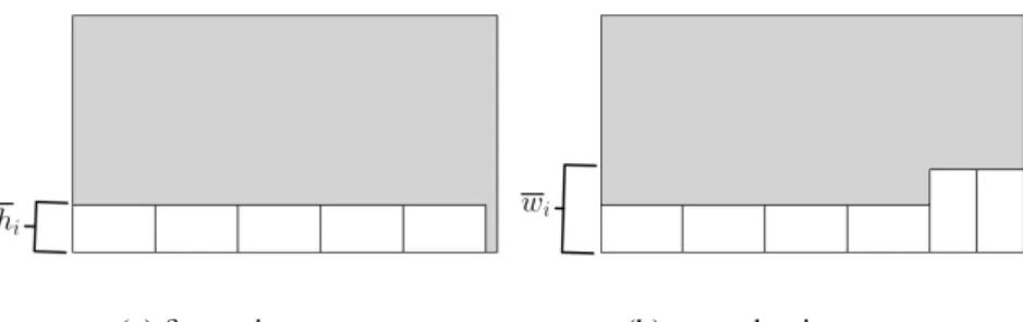
The first strip pattern with item typeicontains exclusively non-rotated items which

means that the height of this strip pattern is equal tohi(Figure 2 - a). The remaining strip patterns

contain at least one rotated item, i.e, the height of theses strip patterns is equal towi, sincehiis

less than or equal towifor alli∈I(Figure 2 - b).

Figure 2 – Strip pattern example

(a) first strip pattern (b) second strip pattern

Each strip pattern jrelated to item typeitakes a vertical space that can be eitherhi

orwi, depending on the presence or absence of a rotated item in the correspondent strip pattern.

The cases with presence of rotated items may lead to symmetrical solutions.

Theorem 2.1 The minimum number of strip patterns associated with item type i that guarantees the maximum area usage of bin l is equal to two.

Proof 2.2 The maximum number of items of type i in a strip pattern containing at least one rotated item is equal tojWl

hi

k

, i.e., the one which contains exclusively rotated items. Hence, any other strip pattern containing both rotated and non-rotated items of type i has a number of items that is less than or equal tojWl

hi

k

.The result is two pattern of interest. One containing exclusively non-rotated items with height equal to hiand another containing exclusively rotated items with height equal to wi.

(22)

Wl=Hl+pfor alll ∈B. This means that setB∗has two times more elements than setB, i.e.,

|B∗|=2|B|=2p.

Letxi jlbe an integer variable associated with the number of strip patterns jof item

typeipacked vertically in binl. Letul be a binary variable associated with the use of binl and

let yibe a binary variable associated with the choice of item type ias the identical item. Let mil =

j

Hl hi

k

be an upper bound forxi jl and letai jl=hiwibi jl be the area associated with strip

pattern jof item typeiwith respect to binl, i.e.,ai,1,l=hiwi

j

Wl wi

k

andai,2,l=hiwi

j

Wl hi

k

_∑

l∈B∗

clul (2.6)

Constraints

hixi1l+wixi2l6Hlul ∀l∈B∗,i∈I (2.7)

xi jl6milyi ∀l∈B∗,i∈I, j={1,2} (2.8)

∑

l∈B∗

∑

_i_∈ 2

∑

j=1

ai jlxi jl>A (2.9)

∑

i∈I

yi=1 (2.10)

ul+ul+p≤1 ∀l∈B (2.11)

xi jl∈N+ ∀l∈B∗,i∈I, j={1,2} (2.12)

yi∈ {0,1} ∀i∈I (2.13)

(23)

The objective (2.6) is to minimize total cost. Constraint set (2.7) limits the sum of heights of the strip patterns packed in binl to the height of the same bin. Constraint set (2.8)

bounds the number of strip patterns of item typeito the choice of the same item as the identical

item. Constraint (2.9) guarantees demand satisfaction and constraint (2.10) forces the choice of one single item type. Constraint set (2.11) limits the choice of a non rotated and a rotated bin to one. Constraint sets (2.12), (2.13) and (2.14) define the domain of the decision variables. The model has, at the worse case scenario, 6np+p+2 constraints, 4npinteger variables andn+2p

binary variables.

ALGORITHMS AND SOLUTION METHODS

In this section, we present two solution procedures for solving the identical item size problem. The procedures deal with the non-rotational case in which the orientation of the identical items is fixed and the rotational case in which orthogonal rotation of items is allowed.

Non-rotational ISP solution method

In modelsM1andM2, the demandAworks as a lower bound, i.e., one can produce more than required, making the two formulations have too many symmetrical solutions. There-fore, the two problems can be approached by fixing the dimensions of the identical items and calculating the maximum area usage for each bin, resulting in a knapsack subproblem, which can be solved for each possible item type. The knapsack subproblem is described as follows.

Sets and indexes

l∈B={1, . . . ,p}: set of bins; i∈I={1, . . . ,n}: set of item types;

Parameters

cl: cost of binl;

al: maximum area usage for binl; A: area demand.

Decision variables

(24)

_∑

l∈B

clul (2.15)

Constraints

∑

l∈B

alul>A (2.16)

ul∈ {0,1} ∀l∈B (2.17)

Taking into consideration the non-rotational case,al can be easily enumerated for a

fixed item heighthand widthwby multiplying the amount

j

Hl h

k

·jWl_wkby the area of the item

h·w. Thereafter, the non-rotational case can be dealt with, by solving the knapsack subproblem

for each possible item type and returning the result with the lowest cost. This knapsack procedure, which we shall refer to asK1, is detailed in Algorithm 1.

Algorithm 1:Knapsack procedure 1

Data:H→array[p],W →array[p],h→array[n],w→array[n],c→array[p],A→float Result:bestCost→float

1 bestCost←∞; 2 fori=1tondo

3 forl=1to pdo

4 al←

j

Hl hi

k

·jWl wi

k

·hi·wi;

5 end

6 cost←knapsackSubProblem(a,c,A);

7 ifcost<bestCostthen

8 bestCost_←cost; 9 end

10 end

Rotational ISP solution method

To deal with orthogonal rotation of items, one must first enumerate the parameteral

by solving a maximization problem. Leth=min{h,w}andw=max{h,w}be the height and width of a predetermined item type. Letbj be the number of items associated with the strip

(25)

Let H andW be the height and width of a predetermined bin, respectively. Letxj

be an integer variable associated with the number of strip patterns jused. Then the following

maximization problem can be solved to find the maximum area usage of a predetermined item type in a predetermined bin. Additionally, b1=

j

W wi

k

and b2=

j

W hi

k

be the number of items associated with non-rotated and rotated strip patterns, respectively (Proposition 2.1).

Objective function

Maximize

_∑

2

j=1

bjxj (2.18)

Constraints

h·x₁+w·x₂6H (2.19)

xj∈N+ ∀j={1, . . . ,2} (2.20)

Objective function (2.18) maximizes the number of items packed. Constraint (2.19) limits the sum of heights of the strip patterns used to the height of the bin and constraint set (2.20) defines the domain of the decision variables.

For the rotational case, the knapsack subproblem (2.15)-(2.17) must be adjusted to include the set of rotated bins. The adjusted knapsack subproblem is defined below.

_∑

l∈B

c_lu_l (2.21)

Constraints

∑

l∈B∗

alul>A (2.22)

ul+ul+p≤1 ∀l∈B (2.23)

(26)

Therefore, the knapsack procedure for solving the rotational problem (K2) is detailed

in Algorithm 2.

Algorithm 2:Solution procedureK2

Data:H→array[2p],W →array[2p],h→array[n],w→array[n],c→array[2p],A→ float

Result:bestCost→float 1 bestCost_←∞;

2 fori=1tondo

3 h←min(hi,wi);

4 w←max(hi,wi);

5 forl=1to2pdo

6 b1←

j

Wl wi

k

;

7 b2←

j

Wl hi

k

;

8 a_l←maximizationSubProblem(b,h,w,H_l);

9 end

10 cost_←adjustedKnapsackSubProblem(a,c);

11 ifcost<bestCostthen

12 bestCost_←cost; 13 end

14 end

Additionally, one can reduce the size of setI (set of possible items) by removing

dominated item types as detailed in Algorithm 3. The result is a new setI∗where|I∗|6|I|.

Theorem 2.2 If a(k)_l is the maximum area usage of bin l with respect to item type k and a(k)_l 6a(i)_l for all l∈B, then item type k is dominated and can be removed from set I of possible items.

Proof 2.3 If a(k)_l 6a(i)_l for all l ∈B then∑_l_∈_Ba(k)_l ul 6∑l∈Ba (i)

l ul. Since ∑l∈Ba (k)

l ul >A and

(27)

Algorithm 3:Dominated items elimination procedure Data:a→array[n, p],I→array[n]

Result:I∗→array[n∗6n]

1 I∗←I;

2 for j=1tondo

3 fori=1tondo

4 win_←False; 5 ifi6= jthen

6 forl=1to pdo

7 ifa(_lj)>a(i)_l then

8 win_←True;

9 breakLoop;

10 end

11 end

12 ifwin = Falsethen

13 remove jfromI∗;

14 breakLoop;

15 end

16 end

17 end 18 end

COMPUTATIONAL RESULTS

In this work, we present some numerical experiments on the two mathematical models and on the two solution procedures with the use of forty randomly generated instances. In order to generate the instances, a set of four bin quantities 10,15,20 and 25 and a set of ten item type quantities 50, 100, 150, 200, 250, 300, 350, 400, 450 and 500 are defined, resulting in a total of 40 instances. The dimensions of the bins and item types are set as a discrete uniform distribution with minimum and maximum of 100 and 200 for the bins and with minimum and maximum of 10 and 60 for the item types. (https://www.researchgate.net/publication/ 322937332_random_instances).

(28)

Python version 3.5 with Pyomo mathematical modeling package (http://www.pyomo.org/) and IBM ILOG CPLEX 12.6.0. The experiments were conducted on a machine with Intel®_CoreTM i5-5200U CPU 2.20GHz x 4 processor, 4GB of RAM, running Ubuntu 16.04 LTS.

For the computational tests we setcl=HlWl, which means that cost is proportional

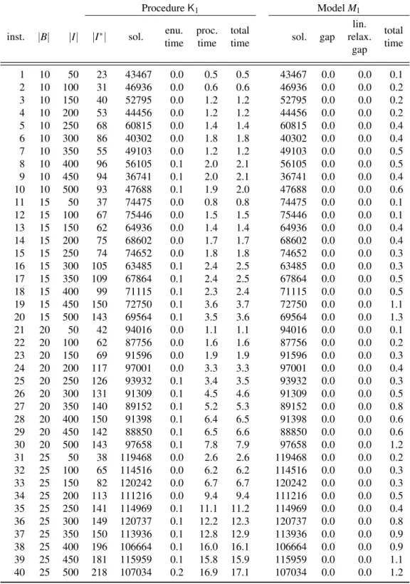
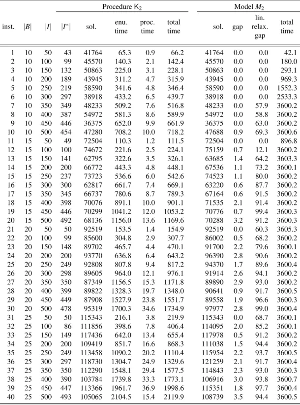
to the area of the bins. Additionally, a time limit of 3600 seconds is imposed to CPLEX for solving models M1 and M2, which will return the relative gap for the cases where time limit is reached. Tables 1 and 2 present the computational results for the cases with and without rotation of items, respectively, including the results for the mathematical models and the solution procedures.

In Tables 1 and 2, the first column indicates the instance which is being evaluated followed by the number of bins and items associated with the respective instance. The forth column shows the number of items after the dominated item elimination procedure. The next four columns are associated with the global optimal solution, enumeration time (including the dominated item elimination procedure), processing time and total time for the solution procedure, respectively. The three last columns show the global optimal solution, relative gap and total computational time for the mathematical model, respectively. Additionally, Figures 5 and 6 display the comparison between the total computational time of the solution procedure and the mathematical model for the non-rotational and rotational cases, respectively.

The enumeration time of procedureK1is, on average, only 1.46% of total computing time, in contrast to 98.61% for K2, as observed in Tables 1 and 2. This large gap between the two procedures is related to the use of mathematical programming for the enumeration procedure by_K2combined with the larger number of dominant patterns. The result is an average computational time ratio of approximately 212 betweenK2andK1, i.e., solution procedureK2 takes, on average, two-hundred and twelve times more computational effort in comparison to_K1. Additionally, on average, the size of the item type set with dominated item elimination|I∗|is 57.91% smaller than the size of set|I|with respect toK1, in contrast to 2.65% with respect to

K2.

(29)

Table 1 – Computational results (non-rotational)

ProcedureK1 ModelM1

inst. |B| |I| |I∗| sol. _timeenu. proc._time total_time sol. gap lin. relax.

gap total time

1 10 50 23 43467 0.0 0.5 0.5 43467 0.0 0.0 0.1 2 10 100 31 46936 0.0 0.6 0.6 46936 0.0 0.0 0.2 3 10 150 40 52795 0.0 1.2 1.2 52795 0.0 0.0 0.2 4 10 200 53 44456 0.0 1.2 1.2 44456 0.0 0.0 0.2 5 10 250 68 60815 0.0 1.4 1.4 60815 0.0 0.0 0.4 6 10 300 86 40302 0.0 1.8 1.8 40302 0.0 0.0 0.4 7 10 350 55 49103 0.0 1.2 1.2 49103 0.0 0.0 0.5 8 10 400 96 56105 0.1 2.0 2.1 56105 0.0 0.0 0.5 9 10 450 94 36741 0.1 2.0 2.1 36741 0.0 0.0 0.4 10 10 500 93 47688 0.1 1.9 2.0 47688 0.0 0.0 0.6 11 15 50 37 74475 0.0 0.8 0.8 74475 0.0 0.0 0.1 12 15 100 67 75446 0.0 1.5 1.5 75446 0.0 0.0 0.1 13 15 150 62 64936 0.0 1.4 1.4 64936 0.0 0.0 0.4 14 15 200 75 68602 0.0 1.7 1.7 68602 0.0 0.0 0.4 15 15 250 74 74652 0.0 1.8 1.8 74652 0.0 0.0 0.3 16 15 300 105 63485 0.1 2.4 2.5 63485 0.0 0.0 0.3 17 15 350 109 67864 0.1 2.4 2.5 67864 0.0 0.0 0.5 18 15 400 99 71115 0.1 2.3 2.4 71115 0.0 0.0 0.5 19 15 450 150 72750 0.1 3.6 3.7 72750 0.0 0.0 1.1 20 15 500 143 69564 0.1 3.5 3.6 69564 0.0 0.0 1.3 21 20 50 42 94016 0.0 1.1 1.1 94016 0.0 0.0 0.1 22 20 100 62 87756 0.0 1.6 1.6 87756 0.0 0.0 0.2 23 20 150 69 91596 0.0 1.9 1.9 91596 0.0 0.0 0.3 24 20 200 117 97001 0.0 3.3 3.3 97001 0.0 0.0 0.4 25 20 250 126 93932 0.1 3.4 3.5 93932 0.0 0.0 0.3 26 20 300 131 91309 0.1 4.5 4.6 91309 0.0 0.0 0.5 27 20 350 140 89152 0.1 5.2 5.3 89152 0.0 0.0 0.8 28 20 400 150 91398 0.1 6.4 6.5 91398 0.0 0.0 0.6 29 20 450 142 88850 0.1 6.5 6.6 88850 0.0 0.0 0.6 30 20 500 143 97658 0.1 7.8 7.9 97658 0.0 0.0 1.2 31 25 50 38 119468 0.0 2.6 2.6 119468 0.0 0.0 0.2 32 25 100 65 114516 0.0 6.2 6.2 114516 0.0 0.0 0.3 33 25 150 82 120242 0.0 6.7 6.7 120242 0.0 0.0 0.3 34 25 200 113 111216 0.0 9.4 9.4 111216 0.0 0.0 0.5 35 25 250 141 114969 0.1 11.1 11.2 114969 0.0 0.0 0.4 36 25 300 149 120737 0.1 12.2 12.3 120737 0.0 0.0 0.8 37 25 350 150 113936 0.1 12.8 12.9 113936 0.0 0.0 0.9 38 25 400 196 106664 0.1 16.0 16.1 106664 0.0 0.0 0.9 39 25 450 181 115959 0.1 15.8 15.9 115959 0.0 0.0 1.1 40 25 500 218 107034 0.2 16.9 17.1 107034 0.0 0.0 1.2

the time limit of 3600 seconds with positive linear relaxation gaps from 12.1% up to 99.4%. From this point we will focus on the analysis of the results for modelM1and procedureK2in detriment to their superior performances in comparison toK1andM2, respectively.

(30)

Table 2 – Computational results (rotational)

ProcedureK2 ModelM2

inst. |B| |I| |I∗| sol. enu._time proc._time total_time sol. gap lin. relax.

gap

total time

1 10 50 43 41764 65.3 0.9 66.2 41764 0.0 0.0 42.1 2 10 100 99 45570 140.3 2.1 142.4 45570 0.0 0.0 180.0 3 10 150 132 50863 225.0 3.1 228.1 50863 0.0 0.0 293.1 4 10 200 189 43945 311.2 4.7 315.9 43945 0.0 0.0 969.3 5 10 250 219 58590 341.6 4.8 346.4 58590 0.0 0.0 1552.3 6 10 300 297 38918 433.2 6.5 439.7 38918 0.0 0.0 2533.3 7 10 350 349 48233 509.2 7.6 516.8 48233 0.0 57.9 3600.2 8 10 400 387 54972 581.3 8.6 589.9 54972 0.0 58.8 3600.2 9 10 450 446 36375 652.0 9.9 661.9 36375 0.0 63.0 3600.2 10 10 500 454 47280 708.2 10.0 718.2 47688 0.9 69.3 3600.6 11 15 50 49 72504 110.3 1.2 111.5 72504 0.0 0.0 896.8 12 15 100 100 74672 221.6 2.5 224.1 75159 0.7 12.1 3600.2 13 15 150 141 62795 322.6 3.5 326.1 63685 1.4 64.2 3603.3 14 15 200 200 66772 443.3 4.8 448.1 67536 1.1 73.2 3600.1 15 15 250 237 73723 536.6 6.0 542.6 74523 1.1 80.0 3600.2 16 15 300 300 62817 661.7 7.4 669.1 63220 0.6 87.7 3600.2 17 15 350 345 66737 780.6 8.7 789.3 67164 0.6 91.5 3600.2 18 15 400 398 70076 891.1 10.0 901.1 71535 2.1 91.4 3600.2 19 15 450 446 70299 1041.2 12.0 1053.2 70776 0.7 99.4 3600.3 20 15 500 492 68136 1156.0 13.6 1169.6 70288 3.2 91.2 3600.3 21 20 50 50 92519 153.5 1.4 154.9 92519 0.0 60.3 3605.3 22 20 100 99 85600 304.8 2.9 307.7 86002 0.5 68.2 3600.2 23 20 150 148 89702 465.7 4.4 470.1 91700 2.2 79.6 3600.1 24 20 200 200 93770 636.8 6.4 643.2 96390 2.8 90.6 3600.2 25 20 250 249 92808 807.8 9.4 817.2 94370 1.7 89.6 3600.4 26 20 300 298 89605 964.0 12.1 976.1 91914 2.6 94.1 3600.2 27 20 350 350 87349 1156.5 15.3 1171.8 89890 2.9 93.0 3600.2 28 20 400 399 89822 1328.3 19.7 1348.0 90641 0.9 91.7 3600.5 29 20 450 449 87908 1527.9 23.8 1551.7 89558 1.9 96.6 3600.3 30 20 500 478 95319 1700.3 34.6 1734.9 97977 2.8 99.0 3600.4 31 25 50 50 115343 216.1 3.8 219.9 115343 0.0 68.7 3600.1 32 25 100 86 111856 398.6 7.8 406.4 114095 2.0 85.2 3600.1 33 25 150 149 117436 642.0 13.4 655.4 117978 0.5 91.2 3600.2 34 25 200 200 109419 851.7 16.6 868.3 111038 1.5 94.4 3600.2 35 25 250 249 113458 1090.2 20.2 1110.4 115954 2.2 93.7 3600.5 36 25 300 297 118730 1304.7 24.9 1329.6 121259 2.1 91.7 3600.4 37 25 350 350 112290 1548.1 29.4 1577.5 114843 2.3 93.0 3600.3 38 25 400 390 103784 1739.8 33.3 1773.1 106916 3.0 93.8 3600.7 39 25 450 447 113366 1961.7 36.9 1998.6 115351 1.8 97.7 3600.4 40 25 500 493 105065 2104.5 15.4 2119.9 108739 3.5 94.4 3600.5

(31)

Figure 3 – Solution for instance 4 -_K1

(a) Bin: 121×152 Item: 10×16 (b) Bin: 181×144 Item: 10×16

Figure 4 – Solution for instance 4 -K2

(a) Bin: 182×164 Item: 20×13 (b) Bin: 127×111 Item: 20×13

(32)

Figure 6 – Computational time (rotational)

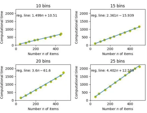
Figure 7 – Computational time x Number of items (M1)

the regression line had an insignificant change. However, for procedure_K2(Figure 8), the impact is clear. The reason for this behavior relies on the fact that the size of setI∗has a direct impact

(33)

Figure 8 – Computational time x Number of items (_K2)

CONCLUSIONS

In this research, a new variant of the two-stage two-dimensional guillotine cutting stock problem was presented. The variant dealt with the case in which items are identical, bins are different in size and the objective is to find the optimum size of the items. This problem was identified in the granite industry during technical visits to a local manufacturer and, to the best of our knowledge; there is no reference of this problem in the available literature.

Mathematical formulations and solution procedures are presented for the cases with and without orthogonal rotation of items. The proposed approaches were evaluated with the use of forty randomly generated instances. The proposed methodology was able to find the global optimum solution for all used instances with acceptable computational time.

For the case without rotation of items, the mathematical model M1 was able to outperform the solution procedure K1 for all instances evaluated. For the case with rotation of item, however, the solution procedure _K2 presented far better results than modelM2. The developed solution procedures dealt with the problem by interactively solving a knapsack subproblem for each possible item size and returning the best solution found. Therefore, the set of possible item sizes is considered finite (or discrete). This assumption was made by virtue of practical operational factors such as cutting precision and standardization of item sizes.

(34)

(35)

REFERENCES

ALVAREZ-VALDES, R.; PARAJON, A.; TAMARIT, J. M. A computational study of lp-based heuristic algorithms for two-dimensional guillotine cutting stock problems.OR Spectrum, Springer, v. 24, n. 2, p. 179–192, 2002.

ALVAREZ-VALDÉS, R.; PARREÑO, F.; TAMARIT, J. M. A branch-and-cut algorithm for the pallet loading problem. Computers & Operations Research, Elsevier, v. 32, n. 11, p. 3007–3029, 2005.

ANDRADE, R.; BIRGIN, E.; MORABITO, R. Two-stage two-dimensional guillotine cutting stock problems with usable leftover.International Transactions in Operational Research, Wiley Online Library, v. 23, n. 1-2, p. 121–145, 2016.

BELOV, G.; SCHEITHAUER, G. A branch-and-cut-and-price algorithm for one-dimensional stock cutting and two-dimensional two-stage cutting. European journal of operational research, Elsevier, v. 171, n. 1, p. 85–106, 2006.

BIRGIN, E. G.; LOBATO, R. D. Orthogonal packing of identical rectangles within isotropic convex regions.Computers & Industrial Engineering, Elsevier, v. 59, n. 4, p. 595–602, 2010. BIRGIN, E. G.; LOBATO, R. D.; MORABITO, R. An effective recursive partitioning approach for the packing of identical rectangles in a rectangle.Journal of the Operational Research Society, Springer, v. 61, n. 2, p. 306–320, 2010.

BIRGIN, E. G.; MORABITO, R.; NISHIHARA, F. H. A note on an l-approach for solving the manufacturer’s pallet loading problem. Journal of the Operational Research Society, Springer, v. 56, n. 12, p. 1448–1451, 2005.

BORTFELDT, A.; JUNGMANN, S. A tree search algorithm for solving the multi-dimensional strip packing problem with guillotine cutting constraint. Annals of Operations Research, Springer, v. 196, n. 1, p. 53–71, 2012.

CHRISTOFIDES, N.; HADJICONSTANTINOU, E. An exact algorithm for orthogonal 2-d cutting problems using guillotine cuts.European Journal of Operational Research, Elsevier, v. 83, n. 1, p. 21–38, 1995.

CINTRA, G.; MIYAZAWA, F. K.; WAKABAYASHI, Y.; XAVIER, E. Algorithms for two-dimensional cutting stock and strip packing problems using dynamic programming and column generation.European Journal of Operational Research, Elsevier, v. 191, n. 1, p. 61–85, 2008.

CUI, Y.; CUI, Y.-P.; YANG, L. Heuristic for the two-dimensional arbitrary stock-size cutting stock problem.Computers & Industrial Engineering, Elsevier, v. 78, p. 195–204, 2014. DYCKHOFF, H. A typology of cutting and packing problems. European Journal of Operational Research, Elsevier, v. 44, n. 2, p. 145–159, 1990.

(36)

FURINI, F.; MALAGUTI, E.; THOMOPULOS, D. Modeling two-dimensional guillotine cutting problems via integer programming.INFORMS Journal on Computing, INFORMS, v. 28, n. 4, p. 736–751, 2016.

GHANDFOROUSH, P.; DANIELS, J. J. A heuristic algorithm for the guillotine constrained cutting stock problem.ORSA journal on Computing, INFORMS, v. 4, n. 3, p. 351–356, 1992. GILMORE, P.; GOMORY, R. E. Multistage cutting stock problems of two and more dimensions. Operations research, INFORMS, v. 13, n. 1, p. 94–120, 1965.

GILMORE, P. C.; GOMORY, R. E. A linear programming approach to the cutting-stock problem.Operations research, INFORMS, v. 9, n. 6, p. 849–859, 1961.

HIFI, M. Exact algorithms for the guillotine strip cutting/packing problem. Computers & Operations Research, Elsevier, v. 25, n. 11, p. 925–940, 1998.

HIFI, M.; NEGRE, S.; OUAFI, R.; SAADI, T. A parallel algorithm for constrained two-staged two-dimensional cutting problems.Computers & Industrial Engineering, Elsevier, v. 62, n. 1, p. 177–189, 2012.

LINS, L.; LINS, S.; MORABITO, R. An l-approach for packing (l, w)-rectangles into rectangular and l-shaped pieces.Journal of the Operational Research Society, Springer, v. 54, n. 7, p. 777–789, 2003.

LODI, A.; MONACI, M.; PIETROBUONI, E. Partial enumeration algorithms for two-dimensional bin packing problem with guillotine constraints.Discrete Applied Mathematics, Elsevier, 2015.

MACLEOD, B.; MOLL, R.; GIRKAR, M.; HANIFI, N. An algorithm for the 2d guillotine cutting stock problem. European Journal of Operational Research, Elsevier, v. 68, n. 3, p. 400–412, 1993.

MORABITO, R.; FARAGO, R. A tight lagrangean relaxation bound for the manufacturer’s pallet loading problem.Stud. Inform. Univ., v. 2, n. 1, p. 57–76, 2002.

MORABITO, R.; MORALES, S. A simple and effective recursive procedure for the manufacturer’s pallet loading problem. Journal of the Operational Research Society, Palgrave Macmillan, v. 49, n. 8, p. 819–828, 1998.

MORABITO, R.; PUREZA, V. A heuristic approach based on dynamic programming and and/or-graph search for the constrained two-dimensional guillotine cutting problem.Annals of Operations Research, Springer, v. 179, n. 1, p. 297–315, 2010.

NTENE, N.; VUUREN, J. H. van. A survey and comparison of guillotine heuristics for the 2d oriented offline strip packing problem.Discrete Optimization, Elsevier, v. 6, n. 2, p. 174–188, 2009.

PUREZA, V.; MORABITO, R. Some experiments with a simple tabu search algorithm for the manufacturer’s pallet loading problem.Computers & Operations Research, Elsevier, v. 33, n. 3, p. 804–819, 2006.

(37)

RIBEIRO, G. M.; LORENA, L. A. N. Lagrangean relaxation with clusters and column generation for the manufacturer’s pallet loading problem.Computers & Operations Research, Elsevier, v. 34, n. 9, p. 2695–2708, 2007.

SILVA, E.; ALVELOS, F.; CARVALHO, J. V. de. An integer programming model for two-and three-stage two-dimensional cutting stock problems. European Journal of Operational Research, Elsevier, v. 205, n. 3, p. 699–708, 2010.

SONG, X.; CHU, C.; NIE, Y. A heuristic dynamic programming algorithm for 2d unconstrained guillotine cutting.WSEAS Transactions on Mathematics, v. 3, p. 230–238, 2004.

STEUDEL, H. J. Generating pallet loading patterns: a special case of the two-dimensional cutting stock problem.Management Science, INFORMS, v. 25, n. 10, p. 997–1004, 1979. SULIMAN, S. A sequential heuristic procedure for the two-dimensional cutting-stock problem. International Journal of Production Economics, Elsevier, v. 99, n. 1, p. 177–185, 2006. VANDERBECK, F. A nested decomposition approach to a three-stage, two-dimensional cutting-stock problem.Management Science, INFORMS, v. 47, n. 6, p. 864–879, 2001. WÄSCHER, G.; HAUSSNER, H.; SCHUMANN, H. An improved typology of cutting and packing problems. European journal of operational research, Elsevier, v. 183, n. 3, p. 1109–1130, 2007.

WEI, L.; TIAN, T.; ZHU, W.; LIM, A. A block-based layer building approach for the 2d guillotine strip packing problem. European Journal of Operational Research, Elsevier, v. 239, n. 1, p. 58–69, 2014.

(38)

3 AK-STAGE TWO-DIMENSIONAL GUILLOTINE CUTTING STOCK PROBLEM

WITH SETUP COSTS

RESUMO

Neste estudo é investigado o problema de corte dek-estágios, no qual é considerado o custo de setupassociado aos estágios de corte. Esta nova variante aparece na indústria do granito, na

qual otrade-off entre o custo de desperdício de material e o custo de operação deve ser avaliado

em cada licitação. Uma formulação matemática pseudo-polinomial com O(23np)variáveis e

O(22np)restrições é apresentada, on qualne psão o número de itens e placas, respectivamente.

Testes computacionais são elaborados em seis instâncias especiais geradas aleatoriamente.

Palavras-chave: Problemas de corte e empacotamento; Programação matemática

ABSTRACT

In this study we investigate the k-stage two-dimensional guillotine cutting stock problem, in

which setup cost associated with cut stages is considered. This new variant appears in the granite industry, in which the trade-off between material waste and operational cost must be evaluated in each bid. A pseudo-polynomial mathematical formulation withO(23np)variables and O(22np) constraints is presented, in which n and p are the number of items and bins,

respectively. Computational tests are performed in six special randomly-generated instances.

Keywords: Cutting and packing problems; mathematical programming.

INTRODUCTION

Cutting and packing problems (CPP) are a class of combinatorial problems widely studied in the past fifty years. A special class of CPP is known as two-dimensional guillotine cutting stock problem in which large rectangular objects (bins) are orthogonally cut from edge-to-edge in order to produce small objects (items). A set of parallel edge-edge-to-edge cuts configures a stage of cut and each stage has an orientation that sequentially alternates between horizontal and vertical starting with the chosen orientation for the first stage.

(39)

cut planning. The first one is associated with the heterogeneity of the stock. According to the analyst, the different sizes of bins makes the planning process more difficult as the number of possible cutting patterns is greater than it would be if the bins were identical. The second difficulty is associated with the trade-off between operational cost and complexity level of a certain cut plan. The operational cost and the complexity are associated with the number of setups required to execute a cut plan.

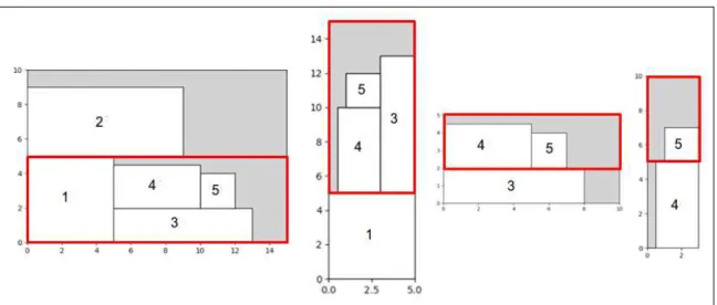
In this specific practical case, the cutting blade performs edge-to-edge cuts with fixed orientation, which means that, every time a new cutting stage is used, a setup (i.e. bin rotation) is required. The problem relies on the fact that setup is significant to the total cost. In Figure 9, e.g., item 5 have a higher setup cost in compare to item 2 as item 5 takes three stages of cutting to be extracted from the bin in contrast to one stage for item 2, as illustrated in Figure 10.

Figure 9 – Four-stage cutting pattern

According to the typology of Wäscheret al.(2007) the problem addressed in this

section is a two-dimensional rectangular Multiple Stock Size Cutting Stock Problem (MSSCSP) with additional constraints related with the types of cuts allowed and additional cost associated with setup. In this particular case, the additional constraints regarding the types of cut allowed is related to orthogonal edge-to-edge cuts, i.e., guillotine cuts.

(40)

Figure 10 – Four-stage cutting procedure

(2001), Alvarez-Valdeset al.(2002), Songet al.(2004), Belov and Scheithauer (2006), Morabito

and Pureza (2010), Furini and Malaguti (2013), Lodiet al.(2015), Andradeet al.(2016) and

Furiniet al.(2016).

AnO(n3)approximation algorithm for the two-dimensional guillotine cutting stock problem is presented by MacLeod et al.(1993). A column generation based approach for a

three-stage two-dimensional cutting stock problem is used by Vanderbeck (2001) with additional constraints related to the cutting process. Later, Alvarez-Valdes et al.(2002) and Cintraet al.

(2008) also present a column generation procedure with the use of dynamic programming. Suliman (2006) presents a three stages sequential heuristic procedure for the two-dimensional cutting-stock problem without guillotine constraint. Belov and Scheithauer (2006) use a branch-and-cut-and-price algorithm for one-dimensional cutting stock problem and two-dimensional two-stage cutting stock problem based on Gilmore and Gomory (1961) and Gilmore and Gomory (1965). Later, Cintraet al.(2008) investigate several two-dimensional guillotine

cutting stock and strip packing problem variants with orthogonal rotation of items.

The unconstrained variant of the two-dimensional unconstrained guillotine cutting is investigated by Song et al.(2004) with the use of dynamic programming. Later, Morabito

and Pureza (2010) presents a heuristic approach based on dynamic programming and and/or graph search for the constrained two-dimensional guillotine cutting problem using a state space relaxation of a dynamic programming formulation of the problem and a state space ascent procedure of sub-gradient optimization type. Lodiet al.(2015) present a heuristic algorithm

(41)

Silvaet al.(2010) propose an integer-programming model for two and three-stage

two-dimensional cutting stock problems considering the input minimization case for the exact and non-exact problems. Later, Furini and Malaguti (2013) present three mixed integer problem models for the two-dimensional two-stage cutting stock problem with multiple stock size with a polynomial, pseudo-polynomial and exponential number of variables, respectively. Andrade

et al. (2016) propose two models for the two-dimensional cutting stock problem with usable

leftovers in which the bins present different size.

Hifi (1998) and later Bortfeldt and Jungmann (2012) propose algorithms for the guillotine strip packing in which the first is a tree search algorithm for the strip packing problem in two and three dimensions and the second is a branch-and-bound and dynamic programming procedure for the two dimensional case. Wei et al. (2014) approach the two-dimensional

guillotine strip packing problem with a block-based layer building in which three known strategies are combined in a single algorithm. For more insight on heuristics for the two-dimensional guillotine strip packing see Ntene and Vuuren (2009).

This paper aims at presenting and solving a new variant of CCP defined as ak-stage

two-dimensional guillotine cutting stock problem with setup cost associated with stages. To the best of our knowledge, this work is the first to address the above-mentioned problem. The rest of this paper is structured as follows: in the next section, a mathematical formulation is presented; in the third section, the computational results are shown. Lastly, in the final section, we present some conclusions and suggestions for future research.

MATHEMATICAL FORMULATION

The following model is an extension of the bin packing modelM1of Andradeet al. (2016). The author deals with two-stage bin packing problems in which items open horizontal spaces inside a bin, known as shelves. The height and width of a particular shelf is equal to the height of the item that opened and the difference between the width of the bin and the widths of the item, respectively. Finally, the remaining items can be packed inside the opened shelves. The model presented in this paper extends this idea for approaching ak-stage cutting stock scenario.

(42)

heights or widths of actual items. In what follows, some notation is introduced for the proposed model.

Sets and indexes

l∈ {1, . . . ,p}: set of bins; i∈ {1, . . . ,n}: set of items;

j∈ {n+1, . . . ,m}: set of dummy items; s∈ {1, . . . ,k}: set of stages;

O(k) ={3,5, . . . ,k}: set of odd stages whenkis odd; O(k) ={3,5, . . . ,k−1}: set of odd stages whenkis even; E(k) ={4,6, . . . ,k}: set of even stages whenkis even; E(k) ={4,6, . . . ,k−1}: set of even stages whenkis odd.

Parameters

Hl: height of binl; Wl: width of binl; cl: cost of binl;

hi: height of item typei; wi: width of item typei;

ds: setup cost related to stages; k: maximum number of stages.

βi: indexes of items sorted in terms of height such thathβ1>hβ2>. . .>hβm;

γi: indexes of items sorted in terms of width such thatwγ1 >wγ2>. . .>wγm;

αi:

        

1, i=1

i, h_β_i 6=h_β_i₋₁∀i=2, . . . ,m

αi−1, hβi =hβi−1∀i=2, . . . ,m

λi:

        

1, i=1

i, wγi6=wγi−1∀i=2, . . . ,m

λi−1, wγi=wγi−1∀i=2, . . . ,m

θi:

        

m, i=m

i, h_β_i 6=h_β_i₊₁∀i=m−1, . . . ,1

(43)

δi:         

m, i=m

i, wγi6=wγi+1∀i=m−1, . . . ,1

δi+1, wγi=wγi+1∀i=m−1, . . . ,1

Decision variables

qjl: 1, if item jopens a first stage shelf in binl; and 0, otherwise;

x(s)_{i jl}: 1, if itemiopens a stagesshelf on stages−1 shelf opened by item jon binl;

0, otherwise;

ul: 1, if binlis used; 0, otherwise.

Objective function

Minimize

p

∑

l=1

clul+ k

∑

s=2 m

∑

i=1 m

∑

j=1 p

∑

l=1

dsx(s)_{i jl} (3.1)

Constraints

m

∑

j=1

hjqjl 6Hlul ∀l∈ {1, . . . ,p} (3.2)

m

∑

i=αj

w_β_ix(_β2)

iβjl6(Wl−wβj)qβjl ∀j∈ {1, . . . ,m},l∈ {1, . . . ,p} (3.3)

m

∑

i=λj hγix

(s)

γiγjl 6

θj

∑

v=1

(h_β_v−hγj)x (s−1)

γjβvl ∀j∈ {1, . . . ,m},l∈ {1, . . . ,p},s∈O(k) (3.4)

m

∑

i=αj wix(s)_β

iβjl6

δj

∑

v=1

(wγv−wβj)x (s−1)

βjγvl ∀j∈ {1, . . . ,m},l∈ {1, . . . ,p},s∈E(k) (3.5)

p

∑

l=1

q_β_il+

_∑

s∈{2}∪E(k)

θi

∑

j=1 p

∑

l=1

x(s)_β

iβjl+

∑

s∈O(k)

δv

∑

j=1 p

∑

l=1

x(s)_γ vγjl=1

∀i,v∈ {1, . . . ,m|βi=γv≤n}

(3.6)

p

∑

l=1

q_β_il+ θi

∑

j=1

x(se)_β iβjl+

δv

∑

j=1

x(so)_γ

vγjl ≤1 ∀l∈ {1, . . . ,p},se∈ {2} ∪E(k),so∈O(k), i,v∈ {1, . . . ,m|βi=γv≥n+1}

(44)

qjl ∈ {0,1} ∀j∈ {1, . . . ,m},l∈ {1, . . . ,p} (3.8)

x(s)_{i jl} ∈ {0,1} ∀i,j∈ {1, . . . ,m},l∈ {1, . . . ,p},s∈ {2, . . . ,k} (3.9)

ul∈ {0,1} ∀l∈ {1, . . . ,p} (3.10)

The objective function (3.1) minimizes the cost which is composed of bin usage cost and setup cost. Constraint set (3.2) ensures that, for each bin used, the sum of heights of the items that open a shelf on the first stage does not exceed the height of the associated bin. Constraint set (3.3) ensures that the sum of the widths of the items that open a second stage shelf on the first stage shelf opened by item jdoes not exceeds the width of the bin on which the

shelves are been opened minus the width of the item j. Constraint set (3.4) ensures that, for each

stages∈O(k), the sum of the heights of the items that open a stagesshelf at the stages−1 shelf opened by item j does not exceed the height of the stages−2 shelf on which item j is

opened minus the height of the item j. Constraint set (3.5) ensures that, for each stages∈E(k),

the sum of the widths of the items that open a stagesshelf at the stages−1 shelf opened by item

jdoes not exceed the width of the stages−2 shelf on which item jis opened minus the width

of the item j. Constraint set (3.6) ensures that the demand of each item is met. Constraint set 3.7

ensures that a dummy item can be used at most one time for each binl and stages. Constraint

sets (3.8), (3.9) and (3.10) define the domain of the decision variables. The model has,O(m2pk) variables andO(mpk)constraints.

The above-described model limits the number of cut stages to the parameterk, which

means that the higher the value ofk, the lower the value of the objective function. To guarantee

the maximum possible number of cut stages, one can set k=m. The result is a model with O(m3p)variables andO(m2p)constraints.

Proposition 3.1 If Zk and Zgare the global optimal solution values for the setup model in which k and g are the maximum number of stages allowed such that k<g, then Zk>Zg.

(45)

Additionally, if all possible dummy items are considered, the total number of dummy items (m−n) will be equal to∑n_i=₂C_inwhich isO(2n), resulting in a pseudo-polynomial model

withO(23np)variables andO(22np)constraints.

(46)

Algorithm 4:Dummy items enumeration procedure Data:H: array[p],W : array[p],h: array[n],w: array[n] Result:m: integer,h: array[m],w: array[m]

1 maxH=max(Hl∀l∈ {1, . . . ,p});

2 maxW =max(Wl∀l∈ {1, . . . ,p});

3 m=n;

4 dh= [null],dw= [null];

5 fori=1ton−1do 6 for j=itondo

7 x←hi+hj,y←wi+wj;

8 ifx6maxH andx∈/dhthen

9 dh+ =x,m+ =1;

10 end

11 ify6maxW andy∈/dwthen

12 dw+ =y,m+ =1;

13 end

14 end 15 end

16 stop=False;

17 N1=size(dh); 18 whilenotstopdo

19 fori=1tondo

20 for j=1toN1do 21 x=hi+dhj;

22 ifx6maxH andx∈/dhthen

23 dh+ =x,m+ =1;

24 end

25 end

26 end

27 ifsize(dh)>N₁then

28 N1=size(dh) 29 else

30 stop=True

31 end

32 end

33 stop=False;

34 N₂=size(dw);

35 whilenotstopdo

36 fori=1tondo

37 for j=1toN2do 38 y=wi+dwj;

39 ify6maxW andy∈/dwthen

40 dw+ =y,m+ =1;

41 end

42 end

43 end

44 ifsize(dw)>N2then 45 N2=size(dw) 46 else

47 stop=True

48 end 49 end 50 h+ =dh;

51 w+ = [0]×N1; 52 w+ =dw;

(47)

In Algorithm 4, lines (1-2) set the maximum height and width of the bins, respectively. Line (4) defines the set of heights and widths of the dummy items as null. Lines (5-15) increment the set of heights and widths of the dummy items by combining the set of heights and widths of the actual items two-by-two, respectively. Lines (16-32) increment the set of heights of the dummy items combining the heights from the same set with the set of heights of the actual items until the set of heights of the dummy items is complete as stated in lines (27-31). Lines (33-49) increment the set of widths associated with the dummy items the same way as defined in lines (16-32) for the heights. Lines (50-53) update the set of heights and widths of the items with the set of heights and widths of the dummy items.

COMPUTATIONAL RESULTS

In this section we perform numerical experiments to analyze the setup model. Six special randomly generated small-scale instances were considered to asset the model (https: //www.researchgate.net/publication/322702826_random_instances). It is important to highlight that medium to large-scale instances are impracticable to be solved by the model proposed and the instances provided by Andradeet al.(2016) did not allow more than two stages for most of

the instances. The bins and items that compose each instance are described at Table 3, in which

pis the number of bins andnis the number of items.

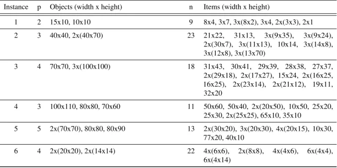
Table 3 – Instances

Instance p Objects (width x height) n Items (width x height)

1 2 15x10, 10x10 9 8x4, 3x7, 3x(8x2), 3x4, 2x(3x3), 2x1 2 3 40x40, 2x(40x70) 23 21x22, 31x13, 3x(9x35), 3x(9x24),

2x(30x7), 3x(11x13), 10x14, 3x(14x8), 3x(12x8), 3x(13x70)

3 4 70x70, 3x(100x100) 18 31x43, 30x41, 29x39, 28x38, 27x37, 2x(29x18), 2x(17x27), 15x24, 2x(16x25, 16x25), 2x(23x14), 2x(21x12), 19x11,

32x20

4 3 100x110, 80x80, 70x60 11 50x60, 50x40, 2x(20x50), 10x50, 25x20, 25x30, 2x(25x25), 65x10, 35x10

5 5 2x(70x70), 80x80, 80x90 13 2x(30x20), 3x(20x30), 4x(20x15), 10x30, 77x20, 40x10

6 4 2x(20x20), 2x(14x14) 22 4x(6x6), 2x(8x8), 4x(4x6), 6x(4x4), 6x(4x14)

(48)

propor-tional to the bin area) and the setup cost is set as a proportionPof the smallest available bin area,

i.e.,ds= (s−2)·P·min{HlWl∀l=1, . . . ,p}(s=2, . . . ,k). Additionally, a low and high setup

cost configuration are taken into consideration, whereP=5% is the cost proportion for the low setup cost configuration andP=20% is the cost proportion for the high setup cost configuration. To evaluate the impact of the maximum number of stages allowed (k) in the solution time, we

considerk={3,4,5}, resulting in six different configurations to be tested.

The models were implemented on python version 3.5 with the use of Pyomo mathe-matical modeling language (http://www.pyomo.org/) combined with IBM ILOG CPLEX 12.6.0 solver. The experiments were conducted on a machine with Intel® CoreTM i5-5200U CPU 2.20GHz x 4 processor, 4GB of RAM, running Ubuntu 16.04 LTS.

Table 4 present the number of dummy items generated by Algorithm 4 for each instance evaluated.

Table 4 – Dummy items

instance number of items number of dummy items total number of items

1 9 19 28

2 23 76 99

3 18 145 163

4 11 33 44

5 13 19 32

6 22 14 36

Results are presented in Tables 5, 6 and 7 fork=3,4 and 5, respectively. In Tables

5 to 7, the first column indicates the instance which is being evaluated followed by the number of dummy items generated. The third column indicate the maximum number of stages used in the solution with low setup configuration. The fourth, fifth and seventh columns present the setup cost, bin cost and total cost (objective) with low setup configuration. Columns eight to twelve show the same information presented in columns three to seven but with respect to the hight setup cost configuration.

(49)

16.6% of the solutions using five stages, 33.3% using four stages and 16.6% using three stages. Furthermore, we evaluate the impact on the computational time when setup cost increases. On average, the computational time with low setup configuration took approximately 15 times more computational effort when compared to the high setup configuration results.

Table 5 – Computational results (k=3)

low setup cost high setup cost

inst. max stages used setup cost bin cost objective solution time max stages used setup cost bin cost objective solution time

1 3 30.0 150.0 180.0 0.19 2 0.0 250.0 250.0 0.17 2 2 0.0 5600.0 5600.0 2.86 2 0.0 5600.0 5600.0 1.44 3 2 0.0 14900.0 14900.0 7.08 2 0.0 14900.0 14900.0 5.27 4 2 0.0 15200.0 15200.0 0.26 2 0.0 15200.0 15200.0 0.32 5 2 0.0 11300.0 11300.0 1.06 2 0.0 11300.0 11300.0 0.48 6 2 0.0 996.0 996.0 6.10 2 0.0 996.0 996.0 3.65

1 3 30.0 150.0 180.0 0.48 2 0.0 250.0 250.0 0.33 2 2 0.0 5600.0 5600.0 6.98 2 0.0 5600.0 5600.0 3.03 3 2 0.0 14900.0 14900.0 20.99 2 0.0 14900.0 14900.0 14.80 4 2 0.0 15200.0 15200.0 3.74 2 0.0 15200.0 15200.0 1.14 5 4 2695.0 7200.0 9895.0 34.81 2 0.0 11300.0 11300.0 3.06 6 4 156.8 800.0 956.8 437.82 2 0.0 996.0 996.0 22.63

(50)

Figure 11 – Solution for instance 4 withk=5 and low setup configuration

(a) Bin 1: 100 x 110

Figure 12 – Solution for instance 4 withk=5 and high setup configuration

(a) Bin 1: 100 x 110 (b) Bin 2: 70 x 60

(51)

CONCLUSIONS

In this research, a new variant of the two-dimensional guillotine cutting stock problem was presented. The variant dealt with thek-stage case in which setup cost related to the stages is

considered. To the best of our knowledge, this research is the first to deal with the new variant. The problem emerged from the granite industry during technical visits to a local manufacturer. A pseudo-polynomial mathematical formulation withO(23np)variables andO(22np)constraints was presented and numerical experiments were conducted with small-scale randomly generated instances using the MIP solver IBM ILOG CPLEX. The model was able to solve with optimality all instances tested in acceptable computational time when a limited number of dummy items was generated. However, to guarantee the global optimal solution, one must enumerate all possible dummy items, which is impracticable even for small scale instances. Moreover, the model can be used to find good initial solutions for heuristic approaches by adding dummy items according to the quality desired for the solution. This concept, to the best of our knowledge, have not being explored by the revised literature.

(52)