Calibration of the maximum carboxylation velocity (Vc
max) using
data mining techniques and ecophysiological data from the Brazilian
semiarid region, for use in Dynamic Global Vegetation Models
L. F. C. Rezende
a*, B. C. Arenque-Musa
b, M. S. B. Moura
c, S. T. Aidar
d, C. Von Randow
a,
R. S. C. Menezes
eand J. P. B. H. Ometto
aaEarth System Science Center, National Institute for Space Research - INPE, Av. dos Astronautas, 1758, Jd. Da Granja, CEP 12227-010, São José dos Campos, SP, Brazil
bLaboratory of Plant Physiological Ecology – LAFIECO, Department of Botany, Universidade de São Paulo – USP, Rua do Matão, 277, Cidade Universitária, CEP 05508-090, São Paulo, SP, Brazil
cDepartment of Agrometeorology, Embrapa Tropical Semiarid, Empresa Brasileira de Pesquisa Agropecuária – EMBRAPA, Rodovia BR-428, Km 152, Zona Rural, CEP 56302-970, Petrolina, PE, Brazil
dDepartment of Plant Ecophysiology, Embrapa Tropical Semiarid, Empresa Brasileira de Pesquisa Agropecuária – EMBRAPA, Rodovia BR-428, Km 152, Zona Rural, CEP 56302-970, Petrolina, PE, Brazil
eDepartment of Nuclear Energy, Universidade Federal de Pernambuco – UFPE, Av. Prof. Luis Freire, 1000, CEP 50740-540, Cidade Universitária, Recife, PE, Brazil
*e-mail: luiz.rezende@inpe.br
Received: August 4, 2014 – Accepted: March 24, 2015 – Distributed: May 31, 2016
(With 6 figures)
Abstract
The semiarid region of northeastern Brazil, the Caatinga, is extremely important due to its biodiversity and endemism.
Measurements of plant physiology are crucial to the calibration of Dynamic Global Vegetation Models (DGVMs) that are currently used to simulate the responses of vegetation in face of global changes. In a field work realized in an area
of preserved Caatinga forest located in Petrolina, Pernambuco, measurements of carbon assimilation (in response to light and CO2) were performed on 11 individuals of Poincianella microphylla, a native species that is abundant
in this region. These data were used to calibrate the maximum carboxylation velocity (Vcmax) used in the INLAND
model. The calibration techniques used were Multiple Linear Regression (MLR), and data mining techniques as the Classification And Regression Tree (CART) and K-MEANS. The results were compared to the UNCALIBRATED model. It was found that simulated Gross Primary Productivity (GPP) reached 72% of observed GPP when using the
calibrated Vcmax values, whereas the UNCALIBRATED approach accounted for 42% of observed GPP. Thus, this work
shows the benefits of calibrating DGVMs using field ecophysiological measurements, especially in areas where field
data is scarce or non-existent, such as in the Caatinga.
Keywords: Dynamic Global Vegetation Models (DGVM), maximum carboxylation velocity (Vcmax), Caatinga, Gross
Primary Productivity (GPP), global changes.
Calibração da velocidade máxima de carboxilação (Vc
max), utilizando
técnicas de mineração de dados e dados de ecofisiologia da região semiárida
brasileira, para uso em Modelos de Vegetação Globais Dinâmicos.
Resumo
A região semiárida do nordeste do Brasil, a Caatinga, é extremamente importante devido à sua biodiversidade e
endemismo. Medidas de fisiologia vegetal são cruciais para a calibração de Modelos de Vegetação Globais Dinâmicos (DGVMs) que são atualmente usados para simular as respostas da vegetação diante das mudanças globais. Em um trabalho de campo realizado em uma área de floresta preservada na Caatinga localizada em Petrolina, Pernambuco, medidas de assimilação de carbono (em resposta à luz e ao CO2) foram realizadas em 11 indivíduos de Poincianella microphylla, uma espécie nativa que é abundante nesta região. Estes dados foram utilizados para calibrar a velocidade
máxima de carboxilação (Vcmax) usada no modelo INLAND. As técnicas de calibração utilizadas foram Regressão Linear
1. Introduction
The semiarid region in Northeastern Brazil covers
844,453 km2 (Brasil, 2014) and it is one of the most
populated in the world and also concentrates the poorest
population of the country (Brasil, 2010). A great portion of the population living in this region relies on agro pastoral activities and natural resources for subsistence. These activities are highly dependent on rainfall, and suffer
setbacks due to adverse weather and recurrent drought cycles. Due to the scarcity of water, much of the soil presents low fertility, particularly regarding the levels
of nitrogen, phosphorus and calcium. Currently, more
than 10% of the semiarid area has suffered a very high
degree of environmental degradation, being susceptible
to desertification (Oyama and Nobre, 2004; Cunha et al., 2013; Santos et al., 2014). According to Sampaio et al.
(2005), the area susceptible to desertification is reasonably defined, with a rate of precipitation by evapotranspiration
less than 0.65. The Caatinga is an exclusively Brazilian biome and is extremely important due to a high biological diversity and the presence of many endemic species (Brasil, 2010). The Caatinga is a relatively poorly studied biome, compared to the other Brazilian biomes, despite the fact
that it covers nearly 11% of the Brazilian territory. In 2012
and 2013 this region experienced one of the most severe drought events in 50 years (Santos et al., 2014). Dynamic
Global Vegetation Models (DGVMs) are important tools for projecting environmental risks (potential consequences of climate change) and fostering discussions about a more
sustainable future of the planet, or in this case of the
Caatinga biome. However, models need calibration in order to be able to provide reliable answers. These models have
a high sensitivity to parameters related to photosynthesis (Lebauer et al., 2013; Dietze, 2014).
The carboxylation velocity parameter (Vcmax) is considered one of the most critical for changes in vegetation in face of global changes. The Vcmax is the measurement
of process by which Rubisco catalyzes RuBP with CO2 to produce the carbon compounds that eventually become
triose phosphates (eg glyceraldeide-3P). Triose phosphates are the building block for sugars and starches. Vcmax has
a direct impact on Gross Primary Productivity (GPP)
(Bonan et al., 2012; LeBauer et al., 2013; Rogers, 2014; Dietze, 2014). Several uncertainties have been observed in the results of DGVM simulations and they tend to underestimate maximum GPP (Bonan et al., 2012; Dietze, 2014). This can be attributed to the lack of databases used for proper Vcmax calibration and the fact that canopy level Vcmax values are used, which are lower than those observed
at the leaf level (Schaefer et al., 2012; Dietze, 2014). Rogers
(2014) noted a wide variation in Vcmax used in models
that had identical PFTs (Plant Functional Types) and they
sought to represent the CO2 uptake of the same biomes,
which is critical due to the role of Vcmax in the carbon cycle. The use of static parameters implies that DGVMs cannot adjust to environmental changes (Smith and Dukes, 2012). Physiological processes are considered the main
sources of uncertainties in these models. However, it is expected that a plant physiology database will enable the
calibration and correction of the models and thus reduce substantially these uncertainties in the next generation of DGVMs (LeBauer et al., 2013; Huntingford et al., 2013; Rogers, 2014; Dietze, 2014).
In this work, the objective is to calibrate the value of
Vcmax used in the INLAND model (Tourigny, 2014) for the
Caatinga biome using carbon assimilation (CO2 curves)
from field measurements. INLAND is derived from IBIS
(Foley et al., 1996; Kucharik et al., 2000). We used the
Multiple Linear Regression (MLR) technique for fitting
Vcmax and the Classification And Regression Tree (CART)
and K-MEANS algorithms to define classifications or
groups of Vcmax values. The results of simulations of the INLAND model using the calibrated Vcmax values were
compared to simulations using an uncalibrated configuration of the model. The goal of this work was to evaluate if the
use of Vcmax measurements for model calibration would improve simulated GPP and NEE.
2. Material and Methods
2.1. Field workThe field work was conducted in a 600 ha area of
preserved Caatinga forest, located in the headquarters of Embrapa Tropical Semiarid in Petrolina, Pernambuco,
during the rainy seasons of February 2013 and 2014, with
a purpose of performing CO2 measurements. The Caatinga
vegetation in this region Petrolina is classified as Savannah Steppe trees and shrubs. This type of Caatinga vegetation
represents 75.72% of the total area of the Caatinga
biome (Brasil, 2007). The soil of the experimental area is
classified as Argisol, which is characterized by low water
retention and poor fertility. Caatinga is characterized by
low annual precipitation and prolonged drought periods (6-8 months each year). The rainy season in Petrolina is
from December to April and the dry season is from May to October. In a data series from CPTEC-INPE covering
14 years (1997-2011), the monthly mean maximum
temperatures reach their highest in November (~ 340C) and the average monthly minimum temperatures reach
não calibrado obteve-se 42% da PPB observada. Assim, este trabalho mostra os benefícios de calibrar DGVMs usando medidas ecofisiológicas de campo, especialmente em áreas onde os dados de campo são escassos ou inexistentes,
como na Caatinga.
Palavras chave: Modelos de Vegetação Globais Dinâmicos (DGVMs), velocidade máxima de carboxilação (Vcmax),
their lowest values in July (~ 20°C). The average monthly rainfall for this period shows that February is the month of highest rainfall (~ 88 mm); and August is the month of lowest rainfall (~ 1 mm). The Poincianella microphylla species (vulgar name: catingueira falsa) was selected
because it has a high occurrence in the Caatinga and it
belongs to the Fabaceae family, which represents 50.63%
of the species in the area (Drummond et al., 2002).
Following a direction (125° transect) and a distance of ~120 m from a meteorological tower (9° 2’ 47.4144” S, 40° 19’ 16.7154” W, altitude: 364.7), 11 individuals of catingueira were selected and geo-referenced using a Global Positioning System (GPS). This direction was selected following a prior study of the tower footprint, as part of Caatinga Flux Project. The heights of these individuals
varied from 1.7 to 4.5 m. Physiological measurements were carried using a photosynthesis and fluorescence analyzer LI-6400 (Li-Cor, Nebraska, USA) and were performed on fully expanded and sun-exposed leaves (one leaf per plant),
directly on the standing plants. Temperature of leaves and
relative humidity of chamber were not controlled and they
varied according to the environmental conditions. The time
of measurements was between 7:00 (am) and 3:00(pm) local
time. In light response curves (A × Photosynthetic Active
Radiation – PAR) the points were: 800, 600, 400, 200, 100,
50, 25 and 0 µmol m–2 s–1 performed under Light Emitting
Diode (LED) source light with blue = 10% and CO2 flux
fixed in 400 µmol mol–1. Some tests were performed for
A × PAR curves and we concluded that plants saturate in
points close to 800 µmol m–2 s–1 (instead 1500 µmol m–2 s–1 that is the most common saturating light intensity for C3
species). We understand that even with a high amount of available light, water limitation makes this species have a more conservative strategy and not “cope well” with high radiation especially in times of the year where soil
moisture is not abundant. The equations used to calculate the assimilation of CO2 (A), stomatal conductance (gs) and
intercellular concentration (Ci) followed Von Caemmerer
and Farquhar (1981). Applying model of non-rectangular hyperbola (Long and Hällgren, 1993) AxPAR curves were
performed in order to identify the plants’ photosynthetic
saturation point.
The curves of photosynthetic response to CO2
intercelullar concentration (AxCi) were performed under LED source light (red-blue, 10% blue) set to a PAR of
800 µmol photons m–2 s–1. CO
2 curves were initiated with a CO2 air concentration of 400 µmol mol–1 (e.g., 400 ppm) and decreased to 300, 200, 100, 50 until 0 µmol mol–1.
In sequence, we injected increasing CO2 values of 400, 600, 900 and 1200 µmol mol–1. Carbon assimilation was estimated according to models of Farquhar et al. (1980),
Von Caemmerer and Farquhar (1981), Farquhar and Von
Caemmerer (1982), Von Caemmerer (2000) and it is expressed as a minimum of three main limitations in the plant capacity
to fix carbon: light limited-rate of photosynthesis (Aj), the limited rate Rubisco- for photosynthesis (Ac) and the triose phosphate limitation in the using for photosynthesis (At) (Equation 1):
A = min (Aj, Ac, At) (1)
It was not considered the triose phosphate limitation,
thus Ac and Aj are estimated by Equations 2 and 3: Ac = ([Vcmax (Ci – Γ*)] / [Ci + Kc (1 + O/Ko)]) – Rd (2)
Where Vcmax is maximum velocity of carboxylation; Ci
is concentration intercellular; Γ* is compensation point of
CO2, Kc is the Michaelis-Menten constant for CO2, Ko is the Michaelis-Menten constant for CO2, O is partial pressure of O2 in equilibrium with its dissolved concentration in chloroplast stroma; Rd is mitochondrial respiration rate in the presence of light.
Aj = ([J max (Ci – Γ*)] / [4Ci + 8 Γ*]) – Rd (3)
Using the initial slope of the net assimilation rate
in relation to Ci (Ci less than 200), it was calculated
a maximum speed of Rubisco enzyme carboxylation (Vcmax) for the results obtained from the limiting equation by the limited rate Rubisco (Ac). The calculation of the maximum rate of electron transport (Jmax) was carried out by solving the equation that describes the points of Aj. The stomatal limitation was quantified by the method
Farquhar and Sharkey (1982), described in details by Long
and Bernacchi (2003).
2.2. Modeling work
The INLAND model uses 12 PFTs and the deciduous
shrub PFT was used for the Caatinga region. Data are
organized in a database (DB) (see Figure 1) and we used
some environmental variables that have good (or reasonable) correlation (or anti-correlation) with photosynthesis, such as leaf-level Vapor Pressure Deficit (VpdL), air temperature (Tair) and Photosynthetically Active Radiation (PARout)
measured in the environment. Despite VpdL being used
as an indicator of water availability, VpdL and soil water content are not always covariant (Beer et al., 2009). We use these variables to get a initial value of Vcmax, which is
modified using a soil water stress factor, following the INLAND model (Equation 4):
Vcmax = Vc x stresstl (4)
where Vc is the Vcmax value obtained from learning
machine (data mining) methods, MLR or UNCALIBRATED defined in INLAND for deciduous shrubs; stresstl is a value calculated by INLAND model from precipitation, radiation and air temperature data (collected in the meteorological
tower) and it varies from 0 to 1. Using the field samples, the inferences were done with MLR and with the CART
and K-MEANS unsupervised clustering methods. After calibration using these methods, the rules of CART and
K-MEANS and the MLR equations were implemented in
the INLAND model. 2.2.1. CART
CART is a method to perform a classification through categorical or discretized variables regression with average
values as output (Breiman et al., 1984). This method was
variable (one value of Vcmax) and it solves a multivariate regression problem. We used the CART implementation
in Matlab software version 7.12. This method has other advantages such as the easiness to interpret the results; low
sensitivity to outliers, ability to handle high dimensionality
data (i.e. data with many attributes), and also to identify the
more relevant parameters; requires little data preparation,
whereas other techniques often need the normalization of data; as well as fast processing time and high accuracy
(Sutton, 2005; Lima et al., 2014).
CART input is a set of chained rules such as “IF THEN
ELSE”, forming a hierarchical structure similar to a
tree. It perates on a database and determines the output parameter class based on input attributes. The components of this structure basically are: nodes - rules that test the
values (or attributes); leaves - the classification itself. Each path in the tree (from root to leaf) corresponds to a classification rule. The attribute space (in this case: VpdL, air temperature and PAR) were partitioned by
binary splitting of the input attributes. Each splitting corresponds to a rule concerning the value of the output attribute, being depicted by a node of the tree. At each node, the left or right branch is chosen according to the
value of the considered input attribute, i.e. according to a
simple less than (equal) or greater than (equal) rule (value comparison rule). In this fashion, at some terminal node a “final” discrete value is assigned to the output attribute.
One of the criteria for choosing the attribute for a node is
the choice of the attribute which has highest information
gain that is realized through entropy estimate (more or
less organized data) (Han and Kamber, 2001). A decision tree has many levels and the same attribute may appear many times in different nodes/levels. A pruning criteria
is adopted in order to avoid overfitting, which renders a tree that is not able to perform classification/regression in
a dataset different from the training set (Han and Kamber, 2001; Witten et al., 2011).
2.2.2. K-MEANS (Clustering)
We used the K-MEANS implementation of Weka software version 3.7.1 released under the GNU General Public License. First the K parameter, which represents the number of groups or cluster to be classified, is determined.
K points are chosen at random as cluster centroids by the algorithm. Instances are assigned to their closest cluster centroid according to a distance function (in our Figure 1. Illustration of the main parts of this work: data acquisition, database implementation, calibration (CART and
case, we apply Euclidean distance). Next the centroid, or
mean, of all instances in each cluster is calculated – this
is the “means” part. These centroids are taken to be new
center values for their respective clusters. Finally, the
whole process is repeated with the new cluster centroids.
Iteration continues until the same points are assigned
to each cluster in consecutive rounds, at which point the cluster centroids have stabilized and will remain
the same thereafter (Witten et al., 2011). The data were
normalized in order to transform values between 0 and 1.
The normalization purpose in this case is that magnitude
of the attribute (for example: PARout) could have larger weight in the distance calculation.
2.2.3. Uncalibrated approach
We used the INLAND parameterization defined for
Vcmax of deciduous shrubs PFTs as 27.5×10⁻⁶ mol m–2 s–1
at 15°C (Kucharik et al., 2000), which is uncalibrated
for Caatinga.
2.2.4. Data input and data for comparison
Additional data sets were used: one as input forcing (meteorological data) and another as environmental variables for comparison between observed data and modeled data. Forcing data were incident short and long wave solar radiation (measured with Kipp & Zonen, Inc., pyranometers and pyrgeometers facing up and down at a height of 9 m from the ground), air temperature and relative humidity (measured with Vaisala, Inc., model HMP 45C-L probe at the same height as the radiation sensors), horizontal wind velocity (measured with R. M. Young Company Wind Sentry anemometers) and rainfall data (collected with a Hydrological Services, Pty Ltd., TB4 rain gauge).
The measured data used for the estimation of GPP and
NEE (as explained in the next section) were hourly time series of incoming and reflected photosynthetically active radiation (PAR), net radiation (Rn), friction velocity (u),
sensible heat flux (H), and latent heat flux (LE). PAR was measured with a Kipp & Zonen PAR-Lite sensor. Rn was
acquired with a Kipp&Zonen NR-Lite net radiometer at
10m above the ground.
2.2.5. Gap-filling of the eddy covariance and
meteorological data
GPP and NEE were estimated through the Eddy Covariance gap-filling and flux-partitioning tool that is provided by the Max Planck Institute for Biogeochemistry (Reichstein et al., 2005; Max Planck Institute for Biogeochemistr, 2014).
This method allows filling missing values in a time series. The gap-filling of the eddy covariance method also considers the co-variation of fluxes with meteorological variables and the temporal auto-correlation of the fluxes
(Reichstein et al., 2005). In this algorithm, three different
conditions are identified: 1) Only the data of direct interest
are missing, but all meteorological data are available;
2) Additionally air temperature or VPD is missing, but radiation is available; 3) Radiation data is also missing. In the final comparison, missing values are not considered
in the evaluation of the results (Reichstein et al., 2005).
3. Results
In this section we show results of field measurements,
model calibration using these measurements and simulations using the calibration.
3.1. Ecophysiological measurements
CO2 response and light response curves were measured in
the field to estimate the vegetation responses in catingueira falsa during two periods: February 4-8, 2013 and February, 23-27, 2014, both during the rainy season. Data shows a negative correlation between Vcmax and VpdL of –0.78 for measurements of CO2 at 400 µmol mol–1.
In the 2014 campaign, four outlying values of Vcmax
were higher than 200 µmol m–2 s–1 (203, 226.3, 226.4 and
211) and were discarded from statistical analysis. However only four points were discarded, we think it is important to register these values because there are few (or quasi no)
data of Vcmax and CO2 curves for Caatinga for comparison
(as shown in Table 1).
3.2. Model adjustment of Vcmax
In this section, we show the regression or calibration
of Vcmax based on simulated values of GPP and NEE.
3.2.1. Calibration with Multiple Linear Regression (MLR)
Using MLR we obtained the following fitting Equation 5:
Vcmax = –109.7 – 38.3 VpdL + 9.75 TempAir – 0.03 PARout (5)
It shows that the attribute of highest weight in the linear regression was VpdL with –38.3; air temperature was second in significance with 9.75 and PARout was very
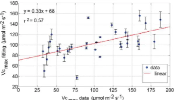
small: 0.03. It has reasonable correlation: 0.57 and root mean squared error of 38.0 (see Figure 2).
3.2.2. Calibration with CART
The CART decision tree learning technique was used to
map the value of Vcmax based on rules related to observed VpdL and air temperature. The inferred rules are illustrated in Figure 3, where each triangle represents a decision level.
For example, in the first level (the top triangle), we can see following decision: – if VpdL is equal or greater than
3.3, Vcmax is classified as 47.0 µmol CO2 m–2 s–1. Each
filled circle is a terminal node, the end of a branch in the
Figure 2. Dispersion of MLR for Vcmax and bar of standard
classification. Otherwise, if VpdL is less than 3.3, the process flows to next decision level (triangle).
After implementing the rules derived from the CART
tree in INLAND, we can see (as shown in Table 2) that
node 2 had a major occurrence (74.9%) of Vcmax of 94.7 µmol CO2 m–2 s–1 and node 4 had less occurrence
(0.11%) for a Vcmax of 159.7 µmol CO2 m
–2 s–1. Two nodes
(1 and 5) with Vcmax less than 48 µmol CO2 m
–2 s–1 had
some significance (both summing 24.9%). Three nodes (3, 6 and 7) had no classified instances.
3.2.3. Calibration with K-MEANS
We choose five centroids/groups, which allows for a
good distribution of discretized Vcmax (with a larger number
of centroids the borders could be very close). Except for
Vcmax, the attribute values used were normalized centroids Table 1. Results of Vcmax estimated through field data and its standard errors of the means (SEM) (n=37).
VpdL
(kPa) ±
Temp.Air
(°C) ±
PARout
(µmol photons m–2 s–1) ±
Vcmax
(µmol m–2 s–1) ±
Vcmax (at 25°C) (µmol m–2 s–1)
±
4.49720 0.34 38.5 0.80 701.6 8.3 37.7 12.4 13.0 7.5
4.43847 0.33 38.4 0.78 1914.4 207.7 77.3 5.9 26.5 5.3
4.02850 0.26 37.8 0.68 963 51.3 60.6 8.7 22.4 6.0
3.27095 0.13 35 0.22 179.5 77.4 159.1 7.4 71.5 2.0
3.46174 0.16 34 0.06 1304 107.4 34.2 13.0 14.6 7.3
2.30124 0.02 31.6 0.33 652.9 0.3 101.5 1.9 60.1 0.1
1.96733 0.07 30 0.59 647.3 0.5 65.3 7.9 44.2 2.4
2.35285 0.01 32 0.26 524.2 20.7 135.8 3.6 77.1 2.9
3.44329 0.16 35.8 0.35 408.7 39.7 40 12.0 16.9 6.9
3.21498 0.12 35.2 0.26 243.3 66.9 143.9 4.9 64.7 0.9
1.24668 0.19 32.4 0.19 184.9 76.5 226.3 18.5 123.2 10.5
1.21799 0.19 33 0.10 316.6 54.8 160.2 7.6 83.3 3.9
1.09090 0.21 32 0.26 632.7 2.9 167.8 8.9 98.5 6.4
1.40622 0.16 32.6 0.16 197.6 74.4 187.6 12.1 101.2 6.9
1.79958 0.10 35.1 0.24 854.7 33.5 226.4 18.5 96.1 6.0
2.64427 0.03 38.5 0.80 1923.3 209.2 41.9 11.7 14.3 7.3
2.42536 0.00 37 0.55 1533.7 145.1 203.1 14.7 72.9 2.2
3.20736 0.12 38.3 0.77 796.5 23.9 144.4 5.0 46.9 2.0
3.38247 0.15 39.3 0.93 1877.2 201.6 32.5 13.3 10.7 6.0
2.97034 0.08 37.1 0.57 484.7 27.2 141.7 4.6 54.9 0.6
2.97897 0.09 35.9 0.37 201.2 73.8 43.7 11.4 17.3 6.8
3.17688 0.12 36.3 0.44 532.9 19.3 179.3 10.8 70.1 1.8
1.17687 0.20 28.3 0.87 220.1 70.7 107.9 0.9 83.8 7.9
1.38237 0.17 31.6 0.33 254.5 65.1 123.2 1.5 75.4 2.6
1.76653 0.10 34.1 0.08 1014.6 59.8 128.5 2.4 59.2 0.0
2.44282 0.00 37.6 0.65 1871.3 200.6 157.7 7.6 60.2 0.1
1.92229 0.08 27.3 1.03 188.5 75.9 107.7 0.9 85.8 4.3
2.05905 0.06 29.1 0.74 227 69.6 51.8 10.1 37.6 3.5
1.83197 0.09 28.8 0.79 222.9 70.3 89.6 3.9 68.4 1.5
1.85148 0.09 28.5 0.84 187.5 76.1 67.6 7.5 52.1 1.1
1.87569 0.09 29.8 0.62 211.3 72.2 90.1 3.8 65.9 1.1
1.89957 0.08 35.2 0.26 291.2 59.0 92.3 3.4 63.1 0.3
2.07286 0.05 30.8 0.46 506.2 23.7 70.3 7.1 44.9 2.3
2.05267 0.06 30.6 0.49 291.6 59.0 134.8 3.4 84.6 4.1
2.20861 0.03 31.6 0.33 556.5 15.4 211 16.0 119.7 9.9
2.32679 0.01 31.4 0.36 460.2 31.2 54.6 9.6 31.4 4.5
(between 0 and 1, as shown in Table 3). Thus these values are proportional to the highest sample of each attribute. We can see that in Group 4 there are high values of VpdL
(0.7393) and air temperature (0.8312), characterizing a hot and dry environment, which is responsible for low Vcmax (45.9 µmol CO2 m–2 s–1). On the other hand, in Group
5 we can see a low VpdL (0.1524), an intermediate air temperature (0.4143) and high Vcmax (148.2 µmol CO2 m–2 s–1). We implemented the results and rules derived of Table 3 and the calculation of distances from instances to centroids in the INLAND model. Table 4 shows the results for each discretized Vcmax (the number of classified
instances and percentage for each group). The group with highest number of classifications was Group 1, with 70.9% of total cases, and the group with less number of cases was Group 5, with 1.31% of total cases.
Both algorithms (CART and K-MEANS) had few cases with high Vcmax (greater than 154 µmol CO2 m
–2 s–1) with
3.44% and 0.11% of total cases, respectively. The node with major number of occurrences (74.9%) with the CART algorithm was Node 2 with Vcmax of 94.7 µmol CO2 m
–2 s–1,
whereas the group with a major number of occurrences (70.9%) using the K-MEANS method was Group 1 with a
Vcmax of 92.5 µmol CO2 m–2 s–1. These values are also closer to a simple mean value of Vcmax (101.01 µmol CO2 m–2 s–1) obtained from the 2013 and 2014 the campaigns, compared to others nodes and groups.
3.2.4. GPP
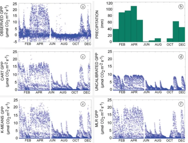
The CART, UNCALIBRATED, K-MEANS and MLR approaches reproduced the GPP variability in comparison
with observed GPP (see Figure 4). However, the results for
the UNCALIBRATED case were highly underestimated
(around 6 µmol CO2 m–2 s–1 in the peak) when observed
GPP was around 25 µmol CO2 m
–2 s–1 in the rainy months
(March-June) (Figure 4a-d). K-MEANS was very reasonable
when the productivity was around 24 µmol CO2 m –2 s–1 in the month of May (Figure 4a-e). For the months of
November and December, K-MEANS was very accurate and GPP reached two peaks with values of ~ 19 µmol
CO2 m–2 s–1 and 23 µmol CO 2 m
–2 s–1 against observations of ~18 µmol CO2 m–2 s–1 and 24 µmol CO
2 m
–2 s–1. Other
approaches (CART and MLR) also had reasonable results for the peaks of November and December, but somewhat less accurate than K-MEANS. In these two months, CART had peaks of 18 and 19 µmol CO2 m
–2 s–1 (Figure 4c);
UNCALIBRATED two peaks of 10 µmol CO2 m –2 s–1 (Figure 4d); MLR 19 and 20 µmol CO2 m–2 s–1 (Figure 4f).
All approaches showed reasonable results during the dry months. A few pulses of precipitation of 4 mm influenced the model between September and October, which allowed for peaks of productivity of 11, 10 and 13 µmol
Figure 3. Vcmax (µmol m–2 s–1) classification tree for the CART algorithm.
Table 2. Number and percentage of occurrences for each Vcmax node using the CART calibration.
Node 1 Node 2 Node 3 Node 4 Node 5 Node 6 Node 7
Occurrences 4165 17361 0 27 1606 0 0
% 17.9 74.9 0 0.11 6.9 0 0
Vcmax 47.0 94.7 59.0 159.7 41.9 113.0 156.6
Table 3. Results of attribute centroids for the K-MEANS algorithm.
Attribute Group 1 Group 2 Group 3 Group 4 Group 5
VpdL 0.1881 0.5743 0.3117 0.7393 0.1524
Temp. of air 0.1033 0.7736 0.3583 0.8312 0.4143
Vcmax 92.5 154.3 76.9 45.9 148.2
Table 4. Classification results of Vcmax using the K-MEANS algorithm.
Group 1 Group 2 Group 3 Group 4 Group 5
Occurrences 18179 882 2478 3755 338
% 70.9 3.4 9.6 14.6 1.3
CO2 m–2 s–1 for CART; 8, 6 and 7 µmol CO 2 m
–2 s–1 for UNCALIBRATED; 11, 10 and 12 µmol CO2 m–2 s–1 for K-MEANS and 10, 11 and 14 µmol CO2 m–2 s–1 for MLR.
All approaches showed high values of productivity between the months of January and February, when observed data show low productivity (~ 5µmol CO2 m
–2 s–1) with
one peak of ~20 µmol CO2 m
–2 s–1. The reason for this initially high productivity is that the stresstl variable
defined in Equation 4 is initialized to 1.0 in a situation of no water stress and evolves through time following
changes in meteorological data such as precipitation and air temperature. None of the approaches produce negative values of GPP. The UNCALIBRATED approach reached
low values of GPP. The Vcmax value (27.5
.10–6 mol m–2 s–1 at 15°C) used in this approach is low when compared to the values reached through the CART, K-MEANS and MLR approaches.
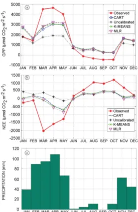
We calculated mean GPP during months March-May,
which is during the rainy season (see Figure 4b), during which a major production is expected compared to other periods of
this year (2011). Notable is the fact that GPP simulated with
the MLR approach (mean of 4.21 µmol CO2 m–2 s–1) was closer to observed GPP (5.99 µmol CO2 m–2 s–1) during this
period. However results for the K-MEANS approach were
nearest to observed GPP. The UNCALIBRATED approach
had the lowest values of Vcmax and the production was
underestimated with a mean value of 2.54 µmol CO2 m –2 s–1. In the analysis of bias and correlation of GPP, all
approaches had a reasonable (good) correlation with observed
GPP data: CART (r2: 0.69), UNCALIBRATED (r2: 0.702), K-MEANS (r2: 0.703) and MLR (r2: 0.716). The totals
of GPP and NEE were calculated monthly (Figure 5). In Figure 5a, it was observed in the productivity peak (April,
2011) that 3 approaches (MLR, K-MEANS and CART) had
values of GPP ~3100, ~3000 and ~3000 µmol CO2 m–2 s–1,
respectively, when observed GPP was of ~4800 µmol
CO2 m–2 s–1. However UNCALIBRATED simulated
low productivity in comparison with observed GPP:
~2000 µmol CO2 m–2 s–1. In the months of July until October,
observed GPP was negative, none of approaches reached
the 0 µmol CO2 m–2 s–1 value. In the months of November and December, three approaches (CART, K-MEANS
and MLR) agreed with observed data (productivity:
~1800 µmol CO2 m–2 s–1). Again, UNCALIBRATED approach (productivity: ~1100 µmol CO2 m–2 s–1) was
lower than observed data. In the analysis of correlation
of GPP monthly totals, all approaches had very good
correlation with observed GPP data: CART (r2: 0.93), UNCALIBRATED (r2: 0.93), K-MEANS (r2: 0.94) and MLR (r2: 0.94).
Figure 4. Data from 2011 - resolution of 1 hour: (a) Observed GPP; (b) Observed precipitation; (c) CART GPP;
Figure 6. Data from 2011 - resolution of 1 hour: (a) observed NEE; (b) PRECIPITATION; (c) UNCALIBRATED NEE;
(d) CART NEE; (e) MLR NEE; (f) K-MEANS NEEE
Figure 5. Monthly means – 2011: (a) GPP; (b) NEE;
(c) Precipitation.
3.2.5 NEE
The CART, UNCALIBRATED, K-MEANS and MLR approaches reproduced the NEE variability compared to observed NEE (see Figure 6). However, all approaches showed a lower amplitude of NEE than observed. UNCALIBRATED results
are more underestimated, with around –5 µmol CO2 m –2 s–1
during the rainy period (March-June/2011), whereas observed NEE was around -20 µmol CO2 m
–2 s–1 (see Figure 6a-c). The K-MEANS approach show results closer
to observed data when the negative amplitude was around
–13 µmol CO2 m–2 s–1 in May (see Figure 6a-f). CART, MLR and K-MEANS reproduce all seasonal variations associated to precipitation throughout the year and the mean difference is around –10 µmol CO2 m–2 s–1 (Figure 6d-f). The difference is larger for UNCALIBRATED than for the other approaches (–15 µmol CO2 m–2 s–1). All approaches
reproduce the negative peaks in November and December (2011). Similar to GPP results, a few precipitation events between September and October influenced the model and negative peaks are observed between the months June and September (2011). All approaches reproduce both phases of amplitude (positive and negative) as observed NEE.
In the analysis of NEE bias and correlation, all approaches
had a reasonable (good) correlation with observed NEE
May when observed data were negative since January until
May. The extreme negative values for approaches CART, K-MEANS and MLR were in May: –695, –720, –844 µmol CO2 m–2 s–1, respectively. UNCALIBRATED approach was negative only in May (–136 µmol CO2 m-2 s-1), Observed
data had negative peak in April (~2000 µmol m–2 s–1) and in May reached ~-1270 µmol CO2 m-2 s-1. In the analysis of correlation of NEE monthly totals, UNCALIBRATED
approach had low correlation and CART, K-MEANS and MLR had good correlation with observed GPP data:
CART (r2: 0.73), UNCALIBRATED (r2: 0.27), K-MEANS (r2: 0.77) and MLR (r2: 0.82).
4. Conclusion
We showed that field measurements of ecophysiological
data can contribute to the calibration of model parameters.
We used data mining techniques to cope with a reduced data sample. Thus, we proposed a discretized Vcmax value, inferred through data mining according to environmental
conditions (dry or wet). After calibration of GPP, the results reached 72% of observed total GPP. CART and K-MEANS approaches had good agreement when the majority of classification cases were using node (74.96%) and group (70.92%) that had nearest mean values of Vcmax (94.7 µmol m–2 s–1 and 92.58 µmol m–2 s–1, respectively).
Also both algorithms (CART and K-MEANS) had few cases with high Vcmax (greater than 154 µmol m
–2 s–1) with
3.4 and 0.1% of total cases, respectively. To our knowledge, this is the first work in Brazil that uses ecophysiological
data collected at semiarid environment for calibration of a
DGVM. This work represents a significant contribution as
a database for the Caatinga biome. We believe that it will
be necessary to expand this database with future works. This task will enable the refinement of the calibration of
DGVMs/Earth system models, since GPP could be affected directly by changes in atmospheric CO2.
Acknowledgments
The authors acknowledge to Dra. Luciana Sandra Bastos
de Souza (Academic Unit of Serra Talhada – UAST -
Federal Rural University of Pernambuco – UFRPE), Gilson Denys (EMBRAPA) and Joemerson Ferreira Damaceno (EMBRAPA) for support in the campaigns.
L.F.C. Rezende and B. C. Arenque-Musa are grateful
to Conselho Nacional de Desenvolvimento Científico e Tecnológico (CNPq) for its support under the processes 142038/2011-3 and 142308/2010-2, respectively. This work has support from Project: Impactos de mudanças climáticas sobre a cobertura e uso da terra em pernambuco: geração e disponibilização de informações para o subsídio a políticas
públicas – FAPESP, Process num. 2009/52468-0 and
Caatinga-FLUX: Monitoramento dos fluxos de energia, CO2 e vapor d’água e da fenologia em área de caatinga – CNPq, Process num. 483223/2011.
References
BEER, C., CIAIS, P., REICHSTEIN, M., BALDOCCHI, D., LAW, B.E., PAPALE, D., SOUSSANA, J.-F., AMMANN, C., BUCHMANN, N., FRANK, D., GIANELLE, D., JANSSENS, I.A., KNOHL, A., KÖSTNER, B., MOORS, E., ROUPSARD, O., VERBEECK, H., VESALA, T., WILLIAMS, C.A. and WOHLFAHRT, G., 2009. Temporal and among-site variability
of inherent water use efficiency at the ecosystem level. Global
Biogeochemical Cycles, vol. 23, no. 2, pp. 1-13. http://dx.doi. org/10.1029/2008GB003233.
BONAN,G.B., OLESON, K.W., FISHER, R.A., LASSLOP, G. and REICHSTEIN, M., 2012Reconciling leaf physiological
traits and canopy flux data: Use of the TRY and FLUXNET
databases in the Community Land Model version 4. Journal of Geophysical Research, vol. 117, no. G02, pp. 1-19. http://dx.doi. org/10.1029/2011JG001913.
BRASIL. Ministério do Meio Ambiente – MMA, 2007. PROBIO: Projeto de Conservação e Utilização Sustentável da Diversidade Biológica Brasileira. Subprojeto: Levantamento da Cobertura Vegetal e do Uso do Solo do Bioma Caatinga. Brasília: MMA. Relatório Final.
BRASIL. Ministério do Meio Ambiente – MMA, 2010. Uso sustentável e conservação dos recursos florestais da CAATINGA.
Brasília: Serviço Florestal Brasileiro.
BRASIL. Ministério do Meio Ambiente – MMA, 2014 [viewed 16 June 2014]. Caatinga [online]. Brasília: MMA. Available from: http://www.mma.gov.br/biomas/caatinga
BREIMAN, L., FRIEDMAN, J.H., OLSHEN, R.A. and STONE, C.I., 1984. Classification and regression trees. Belmont: Wadsworth
Int. Group. 358 p.
CUNHA, A.P.M.A., ALVALÁ, R.C.S., SAMPAIO, G., SHIMIZU, M.H. and COSTA, M.H., 2013. Calibration and Validation of the
Integrated Biosphere Simulator (IBIS) for a Brazilian Semiarid
Region. Journal of Applied Meteorology and Climatology, vol. 52, no. 12. http://dx.doi.org/10.1175/JAMC-D-12-0190.1. DIETZE, M.C., 2014. Gaps in knowledge and data driving uncertainty in models of photosynthesis. Photosynthesis Research, vol. 119, no. 1-2, pp. 3-14. http://dx.doi.org/10.1007/s11120-013-9836-z. PMid:23645396.
DRUMMOND, M.A., KILL, L.H.P., NASCIMENTO, C.E.S.,
2002. Inventário e Sociabilidade de Espécies Arbóreas e Arbustivas
da Caatinga na Região de Petrolina, PE. Brasil Florestal, vol. 21, no. 74, pp. 37-43.
FARQUHAR, G.D. and VON CAEMMERER, S., 1982. Modelling of photosynthetic responses to environmental conditions. In: O.L. LANGE, P.S. NOBEL, C.B. OSMOND and H. ZIEGLER, eds. Physiological plant ecology II. Heidelberg: Springer-Verlag, pp.
550-587. Encyclopedia of Plant Physiology new series, vol. 12B.
FARQUHAR, G.D., VON CAEMMERER, S. and BERRY, J.A., 1980. A biochemical model of photosynthetic CO2 assimilation in leaves of C3 species. Planta, vol. 149, no. 1, pp. 78-90. http:// dx.doi.org/10.1007/BF00386231. PMid:24306196.
FARQUHAR, G.D., SHARKEY, T., 1982. Stomatal conductance and photosynthesis. Annals Review of Plant Physiology. vol. 33, pp. 317-345.
terrestrial carbon balance, and vegetation dynamics. Global
Biogeochemical Cycles, vol. 10, no. 4, pp. 603-628. http://dx.doi. org/10.1029/96GB02692.
HAN, J. and KAMBER, M., 2001. Data mining concepts and techniques. San Franscisco: Academic Press. 548 p.
HUNTINGFORD, C., ZELAZOWSKI, P., GALBRAITH, D., MERCADO, L.M., SITCH, S., FISHER, R., LOMAS, M., WALKER, A.P., JONES, C.D., BOOTH, B.B.B., MALHI, Y., HEMMING, D., KAY, G., GOOD, P., LEWIS, S.L., PHILLIPS, O.L.,ATKIN, O.K., LLOYD, J., GLOOR, E., ZARAGOZA-CASTELLS, J., MEIR, P., BETTS, R., HARRIS, P.P., NOBRE, C., MARENGO, J. and COX, P.M., 2013.Simulated resilience of tropical rainforests to CO2-induced climate change. Nature Geoscience, vol. 6, pp. 268-273http://dx.doi.org/10.1038/NGEO1741.
KUCHARIK, C.J., FOLEY, J.A., DELIRE, C., FISHER, V.A., COE, M.T., LENTERS, J.D., YOUNG-MOLLING, C.,
RAMANKUTTY, N., NORMAN, J.M. and GOWER, S.T., 2000. Testing the performance of a Dynamic Global Ecosystem Model:
water balance, carbon balance, and vegetation structure. Global
Biogeochemical Cycles, vol. 14, no. 3, pp. 795-825. http://dx.doi. org/10.1029/1999GB001138.
LEBAUER, D., WANG, D., RICHTER, K.T., DAVIDSON, C.C. and DIETZE, M.C., 2013. Facilitating feedbacks between field measurements and ecosystem models. Ecological Monographs, vol. 83, no. 2, pp. 133-154. http://dx.doi.org/10.1890/12-0137.1. LIMA, G.R.T., STEPHANY, S., DE PAULA, E.R., BATISTA, I.S., ABDU, M.A., REZENDE, L.F.C., AQUINO, M.G.S. and DUTRA,
A.P.S., 2014. Correlation analysis between the occurrence of
ionospheric scintillation at the magnetic equator and at the southern
peak of the Equatorial Ionization Anomaly. Space Weather, vol. 12, no. 6, pp. 406-416. http://dx.doi.org/10.1002/2014SW001041. LONG, S.P. and BERNACCHI, C.J., 2003. Gas exchange
measurements, what can they tell us about the underlying limitations
of photosynthesis? Procedures and sources of error. Journal of Experimental Botany, vol. 54, no. 392, pp. 2393-2401. http:// dx.doi.org/10.1093/jxb/erg262. PMid:14512377.
LONG, S.P. and HÄLLGREN, J.E., 1993. Measurements of CO2 assimilation by plants in the field and laboratory. In: D.O. HALL, J.M.O. SCURLOCK, H.R. BOLHAR-NORDENKAMPF, R.C. LEEGOOD and S.P. LONG, eds. Photosynthesis and productivity in a changing environment: a field and laboratory manual. London: Chapman and Hall, pp. 129-167.
MAX PLANCK INSTITUTE FOR BIOGEOCHEMISTR, 2014
[viewed 3 February 2014]. Eddy covariance gap-filling & flux-partitioning tool: methods [online]. Available from: http://www. bgc-jena.mpg.de/~MDIwork/eddyproc/method.php
OYAMA, M.D. and NOBRE, C.A., 2004. Climatic consequences of a large-scale desertification in northeast Brazil: A GCM simulation study. Journal of Climate, vol. 17, no. 16, pp. 3203-3213. http://dx.doi.org/10.1175/1520-0442(2004)017<3203:CC OALD>2.0.CO;2.
REICHSTEIN, M., FALGE, E., BALDOCCHI, D., PAPALE, D., AUBINET, M., BERBIGIER, P., BERNHOFER, C., BUCHMANN, N., GILMANOV, T., GRANIER, A., GRÜNWALD, T., HAVRÁNKOVÁ, K., ILVESNIEMI, H., JANOUS, D., KNOHL, A., LAURILA, T., LOHILA, A., LOUSTAU, D., MATTEUCCI, G., MEYERS, T., MIGLIETTA, F., OURCIVAL,
J-M., PUMPANEN, J., RAMBAL, S., ROTENBERG, E., SANZ, M., TENHUNEN, J., SEUFERT, G., VACCARI, F., VESALA, T.,
YAKIR, D. and VALENTINI, R., 2005. On the separation of net ecosystem exchange into assimilation and ecosystem respiration:
review and improved algorithm. Global Change Biology, vol. 11, no. 9, pp. 1424-1439.
ROGERS, A., 2014. The use and misuse of Vc,max in earth system models. Photosynthesis Research, vol. 119, no. 1-2, pp. 15-29. http://dx.doi.org/10.1007/s11120-013-9818-1. PMid:23564478. SAMPAIO, E.V.S.B., ARAÚJO, M.S.B. and SAMPAIO, Y.S.B., 2005.
Impactos ambientais da agricultura no processo de desertificação
do Nordeste no Brasil. XXX Congresso Brasileiro de Ciência do Solo. Revista de Geografia, vol. 22, no 1, pp. 90-112.
SANTOS, M.G., OLIVEIRA, M.T., FIGUEIREDO, K.V., FALCÃO, H.M., ARRUDA, E.C.P., ALMEIDA-CORTEZ, J., SAMPAIO, E.V.S.B., OMETTO, J.P.H.B., MENEZES, R.S.C., OLIVEIRA, A.F.M., POMPELLI, M.F., ANTONINO, A.C.D., 2014. Caatinga, the Brazilian dry tropical forest: can it tolerate climate changes? Theoretical and Experimental Plant Physiology, vol. 26, no. 1, pp. 83-99. http://dx.doi.org/10.1007/s40626-014-0008-0. SCHAEFER, K., SCHWALM, C.R., WILLIAMS, C., ARAIN, M.A., BARR, A., CHEN, J.M., DAVIS, K.J., DIMITROV, D., HILTON, T.W., HOLLINGER, D.Y., HUMPHREYS, E., POULTER, B., RACZKA, B.M., RICHARDSON, A.D., SAHOO, A., THORNTON, P., VARGAS, R., VERBEECK, H., ANDERSON, R., BAKER, I., BLACK, T.A., BOLSTAD, P., CHEN, J., CURTIS, P.S., DESAI, A.R., DIETZE, M., DRAGONI, D., GOUGH, C., GRANT, R.F., GU, L., JAIN, A., KUCHARIK, C., LAW, B., LIU, S., LOKIPITIYA, E., MARGOLIS, H.A., MATAMALA, R.,
MCCAUGHEY, J.H., MONSON, R., MUNGER, J.W., OECHEL, W., PENG, C., PRICE, D.T., RICCIUTO, D., RILEY, W.J., ROULET, N., TIAN, H., TONITTO, C., TORN, M., WENG, E. and ZHOU, X., 2012. A model-data comparison of gross primary productivity: Results from the North American Carbon Program site synthesis. Journal of Geophysical Research, vol. 117, no. G3, pp. 1-15. http://dx.doi.org/10.1029/2012JG001960.
SMITH, N.G. and DUKES, J.S., 2012. Plant respiration and photosynthesis in global-scale models: incorporating acclimation to temperature and CO2. Global Change Biology, vol. 19, no. 1,
pp. 45-63. PMid:23504720.
SUTTON, C.D., 2005. Classification and regression trees, bagging and boosting.Handbook of Statistics, vol. 24, pp. 203-329.
TOURIGNY, E., 2014 [viewed 9 February 2015]. Multi-scale fire modeling in the neotropics: coupling a land surface model to a high resolution fire spread model, considering land cover heterogeneity [online]. São José dos Campos: Instituto Nacional
de Pesquisas Espaciais, 153 p. PhD Thesis in Meteorology. Available from: http://urlib.net/8JMKD3MGP5W34M/3GD37Q2 VON CAEMMERER, S. and FARQUHAR, G.D., 1981. Some
relationships between the biochemistry of photosynthesis and
the gas exchange of leaves. Planta, vol. 153, no. 4, pp. 376-387. http://dx.doi.org/10.1007/BF00384257. PMid:24276943. VON CAEMMERER, S., 2000. Biochemical models of leaf photosynthesis. Canberra: CSIRO Publishing. 165 p.