www.ocean-sci.net/9/855/2013/ doi:10.5194/os-9-855-2013
© Author(s) 2013. CC Attribution 3.0 License.
Ocean Science
Mapping flow distortion on oceanographic platforms using
computational fluid dynamics
N. O’Sullivan, S. Landwehr, and B. Ward
School of Physics and Ryan Institute, National University of Ireland, Galway, Ireland
Correspondence to:B. Ward (bward@nuigalway.ie)
Received: 18 October 2012 – Published in Ocean Sci. Discuss.: 9 November 2012 Revised: 29 July 2013 – Accepted: 9 September 2013 – Published: 17 October 2013
Abstract.Wind speed measurements over the ocean on ships or buoys are affected by flow distortion from the platform and by the anemometer itself. This can lead to errors in di-rect measurements and the derived parametrisations. Here we computational fluid dynamics (CFD) to simulate the errors in wind speed measurements caused by flow distortion on the RVCeltic Explorer. Numerical measurements were obtained from the finite-volume CFD code OpenFOAM, which was used to simulate the velocity fields. This was done over a range of orientations in the test domain from−60 to+60◦in
increments of 10◦
. The simulation was also set up for a range of velocities, ranging from 5 to 25 m s−1 in increments of 0.5 m s−1. The numerical analysis showed close agreement to experimental measurements.
1 Introduction
Accurate measurements of the in situ wind speed are crucial for air–sea interaction studies. In most cases the wind speed is the primary driving force for surface mixing and air–sea exchange, and is therefore typically used as the main or even single parameter for the scaling of air–sea transfer rates. Fast measurements of the three components of the wind speed are used to directly measure air–sea fluxes with the eddy covari-ance method. However, flow distortion occurs when stream-lines circumvent the research platform (see Fig. 1), and can lead to acceleration or deceleration and tilt of the wind vec-tor.
One of the first attempts to define the error associated with flow distortion was a study conducted on the RV Aranda
by Kahma and Lepparanta (1981). An empirical correction factor was developed from the in situ wind speed
measure-ments taken on the ship’s main tower and a bow mast, and by balloon tracking. Kahma and Lepparanta (1981) found that the distortion effect at the ship’s main anemometer was on average 10 % and very sensitive to the wind direction. The measurements taken with an anemometer mounted at a bow boom were however in agreement with free-stream measure-ments taken from balloonracking.
A series of complex potential flow models (i.e steady, in-viscid, incompressible and irrotational flow) was used by Oost et al. (1994) to find corrections for flow distortion for the mean wind speed and the wind stress. For direct eddy co-variance measurements, wind stress can be calculated from the covariance of the horizontal and vertical velocity fluctua-tions.
τ=ρa·w′u′ (1)
Oost et al. (1994) found that the wind stress calculation can also be affected by the tilt of the mean flow away from the horizontal plane and estimated an additional factor of 6 % per degree of tilt for this correction.. Oost et al. (1994) concluded that the numerical correction models were not accurate for the spatial definitions of the structure, and that wind tunnel testing of scaled physical models is more suitable.
Surry et al. (1989) and Thiebaux (1990) used wind tun-nel testing of scaled physical models to estimate the air flow over the Canadian research ships RVHudsonand RV Daw-son. The results showed an increase of 7 % in air flow over anemometer sites located above the ship’s bridge. Brut et al. (2002) used scaled physical models in a water flume, and showed that the mast on which the anemometer is mounted can have a dramatic effect on the airflow measurements.
Fig. 1.Streamlines of distorted airflow by the research vessel’s su-perstructure.
Edson et al. (1998) by comparing their own measurement on board the RVWecomato measurements taken on the research platform RP FLIP when both were within 50 km of each other. The measurements on RP FLIP were considered to be unaffected by flow distortion, because the anemometers were positioned on a long boom away from the superstruc-ture. For relative wind directions between−120 and+120◦
on the bow of the RVWecoma, Edson et al. (1998) found a 15 % overestimation of the wind stress.
Errors in wind speed measurements caused by flow distor-tion are also problematic for the derivadistor-tion of wind-speed-based parametrisations of the air–sea gas transfer velocitykg. These are usually of the form
kg=A·(u10)B. (2)
Griessbaum et al. (2010) used the updated GERRIS code (af-ter Popinet, 2008) to simulate the effect of airflow distor-tion on wind speed measurements on the research vessels RVHakuho Maru and RV Mirai. The estimated errors in the mean wind speed ranged from 4 to+14 %. Depending
on the exponentB in Eq. (2), this can lead to possible bi-ases in the gas transfer velocitykgranging from 30 to 50 %. Griessbaum et al. (2010) concluded that flow distortion ef-fects could explain a part of the huge variance in gas transfer parametrisation: the bias in the transfer velocity varies with both wind speed and with relative wind direction. Therefore the bias in the gas transfer velocitykgis unlikely to be the invariant from one cruise period to another, even if the same platform and anemometer setup is used.
Physical models have limitations but can be used to de-scribe the mean flow distortion. However, in order to model the distortion effects on turbulent fluxes, the turbulent length scale must also be scaled (Popinet et al., 2004). The tur-bulent length scale describes the size of the large energy-containing eddies in a turbulent flow. To define these struc-tures, a sub-scale large eddy simulation (LES) must be em-ployed. The most appropriate available method to achieve
this is to use computational fluid dynamics (CFD), which re-quires a numerical mesh that depends on the research plat-form’s shape. The numerical mesh is used to solve partial differential equations between adjacent cells. CFD modelling for the quantification of flow distortion for wind speed mea-surements was first conducted by Yelland et al. (1998) for the RSSDiscoveryand the RSSCharles Darwin. They used the software package Vectis (a commercial software pack-age which utilises a three-dimensional Reynolds-averpack-aged Navier–Stokes (RANS) solver) to predict the airflow distor-tion at various anemometer sites. The simuladistor-tions predicted that wind speed measurements are biased by approximately 10 % at certain anemometer sites. These simulated predic-tions were used to correct inertial dissipation measurements of the drag coefficient for the four anemometers. This led to the difference in the average drag coefficients being re-duced from a maximum of 20 % for the uncorrected data to 5 % or better for the corrected data (Yelland et al., 1998). Yelland et al. (2002) showed that the modelled flow distor-tion error agreed with the in situ experimental wind speed measurements to within 2 % on various research ships and anemometer locations. These simulations also predicted the vertical displacement of the velocity in order to correct the inertial dissipation method for measuring fluxes. The simu-lation verification was provided by comparing inertial dissi-pation measurements of the wind stress, obtained from in-strument sites that experienced a wide range of vertical dis-placements of air flow (Yelland et al., 2002). These showed a numerically modelled vertical displacement error ranging from 3.8 to−15.2 %.
Popinet et al. (2004) used the more computationally ex-pensive LES solver, which allowed for greater resolution in the turbulent regime of the simulation as well as more defined areas of recirculation on areas in the wake of the ship’s su-perstructure. The Gerris open-source CFD solver was used, which solves three-dimensional, time-dependent Euler equa-tions for an incompressible and inviscid fluid of constant density (Popinet, 2003). This paper involved both experi-mental and numerical data taken from the RV Tangaroa. Popinet et al. (2004) showed that the mean flow character-istics are only weakly dependent on the ship motion, ship speed, wind speed or sea state, but strongly dependent on the relative wind direction. For well-exposed anemometers, the wind speed measurements had a 5 % error, and for anemome-ters in the wake of the ship’s superstructure, there were nor-malised standard deviations of up to 40 %.
CFD has become an established method for correcting the errors associated with direct flux measurements, and this pa-per deals with a CFD flow distortion study for the RVCeltic Explorer. In this paper we report firstly on a computer-aided design (CAD) model of a sonic anemometer mounted on a mast, which represents the physical measurements on the RV
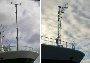
Fig. 2.Photos of the two masts that have been used in this study: left is the single pole mast with a crossbeam for the anemometers. Right shows the triangular lattice mast with the sonic anemometer located on a boom towards the bow.
determine the ideal location for wind speed measurements on the vessel. Furthermore, we investigate the effect of varying pitch angles on the measurement data. Finally, we test two mast designs with three instrumentation setups for the opti-mum experimental design. Our conclusions are provided in the final section.
2 In situ measurements
Measurements were conducted on the RV Celtic Explorer, where, during the period of this project, two masts were used (Fig. 2). The objective of the project was to develop an eddy correlation air–sea flux system for the research vessel. Mi-cro meteorological instrumentation consisted of a Gill R3A sonic anemometer with a Crossbow NAV440 inertial mo-tion unit as well as a Licor LI-7500 CO2/H2O analyser. The mean meteorological measurements were performed using a Young anemometer (wind speed and direction), a Vaisala temperature and humidity probe, a Druck atmospheric pres-sure sensor, an Eppley radiometer (infrared radiation) and an Eppley pyranometer (shortwave radiation). The micromete-orological and mean data were logged on a Moxa UC-7410 embedded computer and a Campbell CR3000 data logger at sample rates of 10 and 0.1 Hz, respectively. These in situ data provided an opportunity to compare the CFD-modelled data described below.
3 CFD modelling
The finite-volume CFD code OpenFOAM 2.0.1 (OpenCFD, 2012) was used to simulate the velocity fields around the RV
Celtic Explorer. OpenFOAM is a C++ library used primar-ily to create executables, known as applications. The
appli-cations fall into two categories: solvers, designed to solve a specific problem in continuum mechanics; and utilities, designed to perform tasks that involve data manipulation. Two standard solvers were used for the simulations presented here:
– PotentialFOAM – a potential flow solver which can be used to generate starting fields for full Navier–Stokes codes and reduces the normal run up time instabilities associated with steady-state simulations (OpenFOAM, 2011).
– SimpleFOAM – this uses the semi-implicit method for pressure-linked equations (SIMPLE) algorithm, which allows for coupling of the Navier–Stokes equations with an iterative procedure (openfoamwiki, 2010). The simulation properties follows the prescribed method of setup conducted by Gagnon and Richard (2010) for the OpenFOAM implementation of the simpleFOAM steady-state algorithm. They were tested against the Ahmed body (a simplified, standardised car body used in CFD testing) wind tunnel data. There are an extensive number of experimental wind tunnel datasets, which are widely used in the valida-tion of external aerodynamics simulavalida-tions in CFD. Testing against these experimental data is considered an acceptable comparison, as the Ahmed body creates defined vortices in its wake region. The Ahmed body model also has an an-gled front section which allows for a defined comparison of lift and drag coefficients. The conclusion from Gagnon and Richard (2010) showed that the chosen simulation’s setup us-ing the simpleFOAM algorithm had a 10 % difference from experimental wind tunnel testing data. A time-varying veloc-ity was applied from 5 to 25 m s−1in steps of 0.5 m s−1at the inlet boundary condition, which is a spatial specification of values at the domain inlet. The temporal discretion scheme (computational time step equations control) between points was defined to allow each velocity input to pass through the domain 10 times (OpenFOAM, 2011).
thus the most significant boundary conditions are the ves-sel surface and the floor surface (the lower boundary of the simulation domain). In accordance with Gagnon and Richard (2010), a classical log-law wall function was applied to the domain floor and vessel’s surface for the turbulence charac-teristics of k(specific kinematic viscosity) and (specific dissipation rate). Thek−shear stress transport (SST) tur-bulence model (Menter, 1993) was used for a turbulent in-tensity of 4 % for all boundary conditions.
A Reynolds number of 108 referenced from Popinet et al. (2004) for airflow at the air–sea boundary layer in the ocean was used to calculate the kinematic viscosity of the fluid. This model is a two-equation eddy viscosity model, and is usable all the way down to the wall through the viscous sub layer. The model was used for its proven reliability in separation zones as well as its ability to blend a good free-stream model with a good boundary layer model (Gagnon and Richard, 2010). The outputted calculations from the simulations contain logs for U(velocity),P (pressure) andk.
The CAD models were generated using the 3-D solid mod-elling software Blender 2.60 (Blender, 2011). Figure 3 shows the generated three-dimensional model and a cross section of the mesh refinement containing hexahedron (hex) and split-hexahedron (split-hex) cells around the RVCeltic Ex-plorer CAD model. Also shown are the four anemometer measurement positions – the bow-mast Gill sonic (BMS), Young’s mean 1 (YM1), Young’s mean 2 (YM2) and the ship bridge deck (SBD). The CAD model was scaled to 1:10, which in turn defined a simulation domain size of 37.85 m×20.2 m×20.2 m for flows directly over the bow. This CAD model scale and model domain size was chosen to give a 1 % blockage area (area ratio between the inlet of the simulation domain and the CAD model) of the in-let section of the wind tunnel by the test geometry as de-scribed by Castro and Robins (1977). This allows for the flow to completely stabilise within the simulation domain. In the case of the RVCeltic Explorer, the size of the domain is also dependent upon the ship’s orientation to the flow. The width of the domain can therefore increase to over 40 m for flows over the ship’s beam. CAD models scaled to 1:1 of
the two masts (Fig. 2) were also created and implemented with the same simulation setup (i.e OpenFOAM numerical solvers, boundary conditions and turbulence model) as the RVCeltic Explorersimulations. A 1 % inlet blockage area was also applied to the domain size and model scale. The mast CAD models were contained within a simulation do-main of 46.9 m×24.9 m×24.9 m. The mast CAD models were also configured with three different instrumentation se-tups, containing different sonic anemometer and Licor gas analyser setups.
Finally, a simulation was implemented where the effect of the pitch angle of the ship on the wind speed determination was evaluated. The CAD model was tilted within the domain through orientations ranging from 0 to 6◦
in steps of 2◦
. The
Fig. 3.RVCeltic Explorermodel with cross section of hex mesh and relative position of experimental anemometers – bow-mast Gill sonic (BMS), Young’s mean 1 (YM1), Young’s mean 2 (YM2) and ship bridge deck (SBD).
domain size and simulation setup remained the same for this model as previously used for the RVCeltic Explorer simula-tions.
The CAD models were imported into OpenFOAM as an interchangeable 3-D file format. In the vessel simulations this was done over a range of orientations in the test domain, from
−60 to+60◦in increments of 10◦, giving 13 model
orienta-tions within the simulation domain. The simulation was set up for 41 different velocities, ranging from 5 to 25 m s−1in increments of 0.5 m s−1.
The vertical orientation of the model was carried out over a range of orientations in the test domain, from 0 to+6◦in
increments of 2◦, giving four model orientations within the
simulation domain. The simulation was also setup for 41 dif-ferent velocities, ranging from 5 m s−1to 25 m s−1in incre-ments of 0.5 m s−1.
The meteorological mast setup comparisons were per-formed for 0–60◦
. This simulation setup was also done for 41 different velocities, ranging from 5 to 25 m s−1in incre-ments of 0.5 m s−1. The meteorological mast setup compar-isons were performed for 2 different mast designs (Mast1 telegraph pole design and Mast2 triangular lattice design) and 3 different instrumentation setups (Gill sonic anemome-ter, Gill sonic anemometer/Licor gas analyser and Campbell sonic anemometer/Licor gas analyser), giving 42 simulations in total. The overall total number of simulations run from all the variations tested was 59.
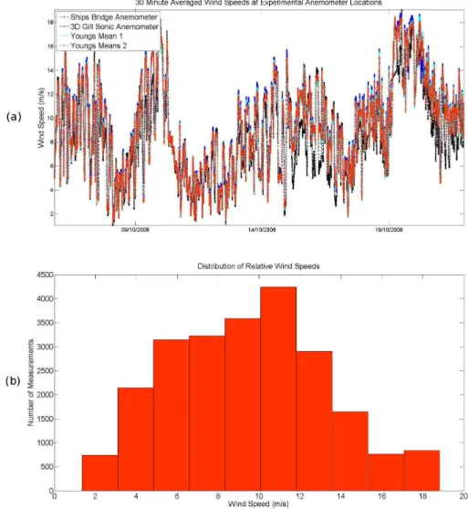
Fig. 4. (a)Thirty-minute-averaged true-wind-corrected measurements for the BMS, YM1, YM2 and SBD anemometers.(b)Histogram of distribution of measured wind speeds for chosen cruise period from the BMS anemometer.
available for jobs. There was a total run time of 14.5 days for the completed code using both computers. Each case was run on 64 parallel processors per case.
4 Results and discussion
In accordance with Popinet et al. (2004), two initial assump-tions were made:
1. The wind speeds measured at different locations should scale linearly with some reference velocity, meaning the fluid flow is essentially independent of the Reynolds number.
2. The averaged velocity depends only on the relative wind direction.
The first assumption is justified as the Reynolds number (∼108based on ship length and 10 m s−1wind speed), and
is well within the asymptotic regime for flow around a solid obstacle (Popinet et al., 2004). We investigate the linearity of the scale of error using highly resolved wind speed runs (see Sect. 4.1).
The second assumption chooses to neglect the influence of the sea conditions as well as ship motion. It is extremely dif-ficult to simulate ship movement (yaw, pitch and roll), which leads to large computational costs. We do, however, investi-gate flow for various fixed pitch angles (see Sect. 4.3).
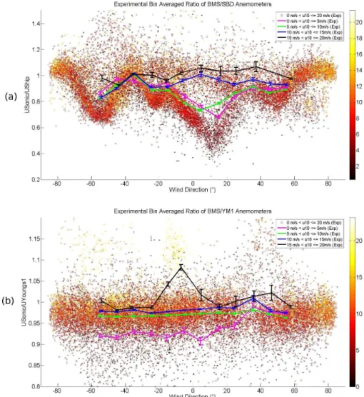
Fig. 5. (a)Experimental bin-averaged wind speed line plots between the BMS and the SBD anemometers over a range of direction from−60
to+60◦, also with experimental scatter plot of full wind speed range and standard deviation error bars.(b)Experimental bin-averaged wind
speed line plots between the BMS and the YM1 anemometers over a range of direction from−60 to+60◦, also with experimental scatter
plot of full wind speed range and standard deviation error bars.
BMS anemometer location to the SBD anemometer loca-tion of 1.28 m s−1. From the BMS anemometer to the YM1 anemometer a mean difference of 0.27 m s−1is recorded. In Fig. 4b, the distribution of velocities showed a lack of data at wind velocities greater than 15 m s−1.
The scatter plot Fig. 5a shows the ratio of experimen-tal 1 min averaged wind speeds from the BMS and the SBD anemometer with respect to the wind direction. Also shown are the bin-averaged data for different wind speed ranges. Figure 5a shows how the change in wind speed af-fects the experimental ratio in measurements between the two anemometers, and that increased distortion effects oc-cur at 10 and−60◦
to the bow. This gives a representation of the wind speed dependence (i.e the deviation of flow distor-tion error scaling from linearity as the measured wind speed increases), and also shows that the highest level of the flow distortion ranges from−5 to+30 %. As the orientation tends
towards the negative direction, a higher distortion error can be seen because of the recirculation caused by a crane which was mounted on the port-side of the vessel. However, this is not the case in the positive wind direction, as is evident in Fig. 5a.
Figure 5b shows the ratio of experimental 1 min averaged wind speeds from the BMS anemometer and the YM1 star-board anemometer (refer to Fig. 3). Here the ratio decreases as a function of wind speed (i.e. the ratio tends towards 1 as the wind speed increases). From this plot, the magnitude of the flow distortion error range was 5 to 10 %.
4.1 Vessel simulations
The vessel simulations were carried out over a range of ori-entations from−60 to+60◦in increments of 10◦. The
Fig. 6. (a)Flow speed over the ship for−60 and+60◦to the bow for a steady-state input stream of 25 m s−1.
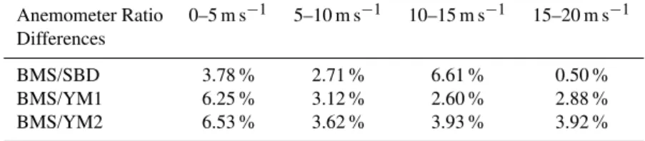
Table 1.Mean differences between numerical and experimental anemometer ratio bin-averaged data in Fig. 8.
Anemometer Ratio 0–5 m s−1 5–10 m s−1 10–15 m s−1 15–20 m s−1
Differences
BMS/SBD 3.78 % 2.71 % 6.61 % 0.50 %
BMS/YM1 6.25 % 3.12 % 2.60 % 2.88 %
BMS/YM2 6.53 % 3.62 % 3.93 % 3.92 %
to 25 m s−1in increments of 0.5 m s−1. Cross-sectional con-tour plots for −60 and +60◦ inflow to the bow are shown
in Fig. 6. These plots show the change in the velocity pro-file for the associated change in direction produce different wake structures in front of the bow. It can be seen for−60◦
(Fig. 6a) that there is a higher gradient of turbulence in the wake of the bow mast. This is also apparent in the exper-imental results shown in Fig. 5a. This is due primarily to the presence of a bow-deck crane on the port side causing increased distortion effects. This verifies the validity of the simulation results as spatially accurate to the physical reality of the experimental results.
A free-stream undistorted measurement was unavailable from the current dataset. In previous works (e.g. Popinet et al., 2004), a reference measurement location was taken as the free-stream undistorted flow measurement (measure-ments of wind speed external to a research vessel are almost impossible to attain). Thus, in order to validate the simula-tions directly from the experimental measurements, a ratio method between chosen anemometers was conducted follow-ing the approach of Popinet et al. (2004). The comparison of the ratio between simulated wind speeds from a refer-enced location and another location in the numerical domain should predict the ratio in experimental measurements over this same space, thus giving an estimate of the accuracy of the simulations to predict a free-stream velocity occurring away from the vessels superstructure. This method is valid due to the fact that relative position of the anemometers does not change in time or space. The ratio across the prescribed anemometer locations was calculated in the simulation re-sults. Figure 7 shows CFD velocities of flow onto the bow ranging from−60 to+60◦.
Figure 7a and b respectively show the ratio between the BMS anemometer and the YM1/2 starboard/port
anemome-ters. The plots show peaks in the simulated error as the in-flow direction aligns with the vertical (T-bar) section of the mast (see Fig. 3), thus causing elevated distortion since the instrument measurement location is in its wake. This is also apparent in Fig. 5b, where a similar range of errors (−1 to 10 %) is present, and also contains the same peak in the neg-ative direction. In Fig. 7c the predicted errors between the BMS anemometer and the SBD anemometer show elevated distortion in the negative direction as a result of the bow-deck crane. Comparing Fig. 7c to Fig. 5a, the same range of errors can be seen. In Fig. 7d we see the surface plot predic-tion of errors for the BMS anemometer locapredic-tion, with respect to the difference from the free-stream velocity, which was taken from the model output for a position 20.5 m upstream of the bow (this is the distance between the BMS and SBD anemometers in Fig. 3).
Fig. 7.Surface plot corrections for ratios between (a)BMS and
YM1 starboard, (b) BMS and SBD, (c) BMS and YM2 port
anemometer(d)BMS and free-stream velocity.
scales upwards). Figure 7d corresponds to Fig. 8d, where the error found from the evaluated surface plot to free stream was extracted from the measured BMS anemometer. This gives a corrected plot of the data (in black) for the duration of the chosen cruise period. The plots show a correction range from 2.4 to −1.0 m s−1, with a root-mean-square value of 0.43 m s−1.
Fig. 8.Bin averages of the measured and modelled wind speed
ra-tios as a function of the relative wind direction for(a)BMS and
YM1 anemometers(b)BMS and YM2 anemometers(c)BMS and
SBD anemometers individual measurements are shown as scatter
plot with the wind speed as color code.(d)Time series of BMS and
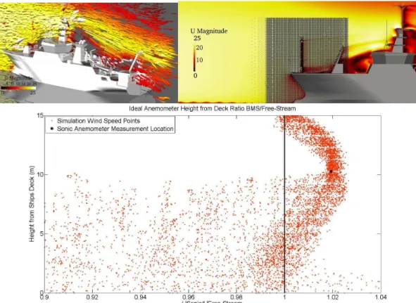
Fig. 9.Top left: cross-sectional velocity vector plot from 5 to 25 m s−1. Top right: grid location for determination of optimised position of the BMS. Bottom: ratio of BMS anemometer to free stream for the data points in the grid above. The black dot indicates the current location of the BMS anemometer.
4.2 Ideal anemometer locations
A vector plot of the velocity profile at 0◦
inflow to the bow is shown in Fig. 9a. This plot was used to define the areas of highly deviated airflow, showing high distortion in the wake of any deck-mounted structure. Deviations from the mean flow and recirculation areas can be seen upwind of the bridge deck. Highly deviated areas with recirculation can also be seen in the wake of the bridge deck. This describes the opti-mum area for positioning of anemometers, which should be as far towards the bow as possible, and facing into the mean free-stream airflow. In Fig. 9b, there is a high-resolution grid (20 955 points) within this defined area, where velocity cal-culations were recorded for each point. The ratio to free-stream velocity for the chosen points ahead of the mast posi-tion were plotted for change in height (Fig. 9c). This shows that the BMS anemometers current position is within a wake region caused by a forward velocity gradient from the bow; therefore the height should ideally be increased to >14 m. For the conditions of this numerical experiment (i.e. 0◦
wind direction at 25 m s−1), the least distorted location for the anemometer was found to be at the bow, close to the deck of the ship. However, this location would likely be different for different flow conditions. The most accurate velocity po-sition outside of this acceleration zone shows that the BMS
anemometer should be placed 3.2 m ahead of the bow and higher than 14 m above the ship’s deck.
4.3 Vertical orientation
Numerical experiments were conducted for pitch angles from 0 to 6◦ in increments of 2◦ for velocity ranges of 5 to
25 m s−1. Figure 10a shows high-resolution velocity plots for a wind input of 25 m s−1and for a model tilt angle of 0◦and
6◦
along itsy axis. What is most striking is the change in the velocity profile across the length of the ship. Focussing on the BMS probe location (Fig. 10b), the effect of changing the ship’s pitch angle is shown. The vertical component of the wind is most sensitive to the change in pitch angle (not shown). The vertical orientation of the ship effectively cre-ates a larger area of blockage with increasing pitch angle, resulting in a maximum distortion effect of 2.5 % at a high wind speed of 20 m s−1.
4.4 Meteorological mast comparison
Fig. 10. (a)Flow speed over the ship for 0◦ and+6◦tilt for a steady-state input stream of 25 m s−1.(b) Modelled ratio from BMS to
undisturbed flow over 5 to 25 m s−1for tilt angles of 0◦, 2◦, 4◦and 6◦.
simulations were performed for a 0–60◦
bow-on wind. In Fig. 11 is shown velocity magnitude profiles around Mast1 and Mast2, each with a Campbell sonic anemometer and Licor LI7500 gas analyser. The wake structure from Mast2 has a greater influence on instrumentation downstream, whereas Mast1 has a more predictable gradient of turbulence in the wake of the design, which allows for a simpler correc-tion. However, Mast1 design has a higher vertical turbulent gradient due to the lack of open sections which would allow for wind to pass through the design.
A cross-sectional vector plot of the airflow divergence for thexdirection uniform inflow velocity is shown in Fig. 12. This was scaled by the measured vertical component of the inflow velocity. Highly distorted wind magnitudes can be seen in the vertical direction of the plot. Anemometer measurement locations positioned directly above the control boxes can be highly affected due to the recirculation caused by the instrumentation. The Campbell sonic anemometer and Licor gas analyser setup position ahead of this vertical vec-tor field is nearly in free stream, defining that positions ahead of this field have little effect from the instrumentation boxes. Comparison of mast geometries was also conducted to al-low for a future comparison with the effects of the new mea-surement system deployed on the RVCeltic Explorerwhen sufficient experimental data are obtained. The developed dif-ferences in the mast geometries can then be applied to the
RV Celtic Explorer simulations containing the Mast1 de-sign. This was conducted due to the complex geometry of the Mast2 design, which would have been computationally expensive in comparison to the Mast1 design and also due to the limited amount of experimental data currently available.
5 Conclusions
It has been established that the OpenFOAM simpleFOAM algorithm shows close agreement with experimental wind speed measurements and can be used as a valid correction for flow distortion over oceanographic platforms. It has shown a close prediction of flow distortion errors to within 12 % of experimental results and predicts the same scale of errors across each space tested. This correlates with the statement of Gagnon and Richard (2010) that the simpleFOAM algo-rithm had a 10 % mean ratio to experimental testing.
Fig. 11.Modelled velocities for each of the two masts for an input
velocity of 25 m s−1
Fig. 12.Cross-sectional velocity vectors scaled from 5 to 25 m s−1
and 0◦.
and YM1. Therefore, over a small space, the prediction of er-ror using an averaged steady-state model is not appropriate, and a sub-scale time-dependant LES model should be used to improve accuracy. This defines also that for the eddy cor-relation calculations, a more accurate LES model should be used to reduce the errors in correcting the wind speed mea-surements used in these calculations.
It has also been found that for a highly accurate correc-tion model, a discrete seleccorrec-tion of inflow direccorrec-tions should be simulated. Higher scatter has been shown to develop in cer-tain orientations as a direct effect of a crane being mounted
on one side of the bow deck. In high-wind-speed situations, the crane causes recirculation and higher errors, which is ap-parent in both numerical and experimental results.
Previous research (e.g., Popinet et al., 2004; Yelland et al., 2002) has correctly concluded that wind direction is the dom-inant factor in flow distortion errors for micrometeorological measurements on research vessels. Our results show that the magnitude of the wind speed is also a quantity of importance, which shows a deviation of flow distortion error scaling lin-early by up to 5.6 % at wind speeds above 5 m s−1. It can also be concluded that wind speed dependence, shown both numerically and experimentally, increases as the wind speed increases above 5 m s−1. We have also found that the flow distortion does not scale linearly with increasing wind speed. The results of the mast simulations indicate that the effects of a more complex geometry give more distortion effects and errors in wind speed estimates. These simulations also show a consistency that is apparent in all the performed simula-tions. High wind speeds tend to have lesser distortion effects. The two simulated mast geometries showed that a more ap-plicable design would be a telegraph pole design with as little blockage as possible to the inflow wind stream. In the future, an optimised design will be developed for deployment and testing.
The comparison between different instrumentation se-tups showed the 3-D Campbell sonic anemometer to have less distortion effects than the 3-D Gill sonic anemometer. This is due primarily to its sampling probe window being ahead of the device, thus causing less impact on the mean airflow. With additional instrumentation positioned beside the anemometer, e.g. a Licor LI-7500 gas analyser, it was found that the best position for sampling is in the wake of the anemometer. This will allow for measurements at the anemometer location to be unaffected by the instrument’s blockage. An evaluation of the Licor LI-7500 dry box also suggested that anemometers positioned directly above dry boxes can be highly affected. This is due to the recircula-tion, and our results suggest that they need to be positioned more than 1.5 m above the dry boxes for unaffected airflow.
The ideal location for the BMS anemometer was found to be as far as possible from the superstructure of the vessel and outside of its wake. It was found that the ideal location of the BMS anemometer for the RVCeltic Explorerwas 3 m ahead of the bow and at an elevation 14 m above the bow deck in order to reduce the distortion effects to 4 %.
the wind speed at low inflow velocities, thus causing higher lift and higher distortion.
Acknowledgements. This research is supported by the Irish Research Council for Science, Engineering and Technology via the Enterprise Partnership Scheme Postgraduate Scholarship Programme, grant number EPSPG/2011/249, and the EU FP7 project CARBOCHANGE under grant agreement no. 264879. S. Landwehr was supported by Science Foundation Ireland under grant 08/US/I1455.
Edited by: A. Sterl
References
Blender: 3D modeling software, version 2.60, 2011.
Brut, A., Butet, A., Planton, S., Durand, P., and Caniaux, G.: In-fluence of the airflow distortion on air–sea flux measurements aboard research vessels: Results of physical simulations applied to the EQUALANT99 experiment, J. Amer. Meteor. Soc., 15, 147–150, 2002.
Castro, I. P. and Robins, A. G.: the flow around a surface mounted cube in uniform and turbulent streams, J. Fluid. Mech., 79, 307– 335, 1977.
Edson, J. B., Hinton, A., Prada, K. E., Hare, J. E., and Fairall, C. W.: Direct covariance flux estimates from mobile platforms at sea, J. Atmos. Ocean. Technol., 15, 547–562, 1998.
Gagnon, L. and Richard, J. M.: Parallel CFD of a prototype car with OpenFOAM, Tech. rep., Dept of Mech. Eng., Laval University, Québec, Canada, 2010.
Griessbaum, F., Moat, B. I., Narita, Y., Yelland, M. J., Klemm, O.,
and Uematsu, M.: Uncertainties in wind speed dependent CO2
transfer velocities due to airflow distortion at anemometer sites on ships, J. Atmos. Chem. Phys., 10, 5123–5133, 2010, http://www.atmos-chem-phys.net/10/5123/2010/.
Kahma, K. K. and Lepparanta, M.: On errors in wind speed obser-vations on R/V Aranda, J. GeoPhysica, 17, 155–165, 1981. Menter, F. R.: Zonal Two Equation k-Turbulence Models for
Aero-dynamic Flows, J. American Institute of Aeronautics and Astro-nautics, 93, 1993.
Oost, W. A., Fairall, C., Edson, J., Smith, S., Anderson, R., Wills, J., Katsaros, K., and DeCosmo, J.: Flow distortion calculations and their application in HEXMAX, J. Atmos. Ocean. Technol., 11, 366–386, 1994.
OpenCFD: OpenFOAM flow solver, version 2.0.1, 2012.
OpenFOAM: OpenFOAM Users Guide 2009, version 1.6, http: //foam.sourceforge.net/doc/Guides-a4/UserGuide.pdf/,(last ac-cess: 12 September 2012), 2011.
openfoamwiki: The Simple algorithm in OpenFoam, http:// openfoamwiki.net/index.php/, (last access: 21 December 2012), 2010.
Popinet, S.: Gerris: A tree-based adaptive solver for the incompress-ible Euler equations in complex geometries, J. Comput. Phys., 190, 572–600, 2003.
Popinet, S.: The Gerris Flow Solver, version 1.2.0, 2008.
Popinet, S., Smith, M., and Stevens, C.: Experimental and numeri-cal study of the turbulence characteristics of airflow around a re-search vessel, J. Atmos. Ocean. Technol., 21, 1575–1589, 2004. Souza, A.: How to understand Computational Fluid Dy-namics Jargon, http://www.nafems.org/downloads/edocs/how_ to_understand_cfd_jargon-nafems.pdf, (last access: 8 Octo-ber 2012) 2005.
Surry, D., Edey, R. T., and Murley, I. S.: Speed and direction correc-tion factors for shipborne anemometers, Tech. rep., University of Western On-tario, London, ON, Canada, 1989.
Thiebaux, M. L.: Wind tunnel experiments to determine cor-rection functions for shipborne anemometers, Tech. rep., Beford Institute of Oceanographyo, Dartmouth, NS, Canada, 1990.
Yelland, M., Moat, B., Taylor, P., Pascal, R., Hutchings, J., and Cornell, V.: Wind stress measurements from the open ocean cor-rected for airflow distortion by the ship, J. Oceanogr., 28, 1511– 1526, 1998.