Comparison of different rules to deal with incomplete information: perspectives of mediation

(1)

Instituto de Engenharia de Sistemas e Computadores de Coimbra

Institute of Systems Engineering and Computers

INESC - Coimbra

Paula Sarabando,

Luis C. Dias

Comparison of different rules

to deal with incomplete information:

perspectives of mediation

No. 2

2009

ISSN: 1645-2631

Instituto de Engenharia de Sistemas e Computadores de Coimbra

INESC - Coimbra

Rua Antero de Quental, 199; 3000-033 Coimbra; Portugal

www.inescc.pt

(2)

(3)

Comparison of different rules to deal with incomplete

information: perspectives of mediation

Paula Sarabando

INESC Coimbra and Departamento de Matemática, Instituto Superior Politécnico de Viseu Campus Politécnico de Viseu, 3504-510 Viseu, Portugal.

e-mail: psarabando@mat.estv.ipv.pt

Luís C. Dias

INESC Coimbra and Faculdade de Economia da Universidade de Coimbra Av Dias da Silva 165, 2004-512 Coimbra, Portugal.

e-mail: ldias@inescc.pt

February 10, 2009

Abstract

In bilateral Negotiation Analysis, the literature often considers the case with complete information. In this context, since the value (or utility) functions of both parties are known, it is not difficult to calculate the Pareto frontier (or efficient frontier) and the Pareto efficient solutions for the negotiation. Thus rational actors can reach agreement on this frontier. However, these approaches are not applied in practice when the parties do not have complete information. Considering that the additive value (or utility) function is used, often it is not easy to obtain precise values for the scaling weights or the levels’ value in each issue. We compare four decision rules that require weaker information, namely ordinal information on weights and levels, to help a mediator suggesting an alternative under these circumstances. These rules are tested using Monte-Carlo simulation, considering that the mediator would be using one of three criteria: maximizing the sum of the values, maximizing the product of the excesses regarding the reservation levels, or maximizing the minimal proportion of potential. Simulations asses how good is the alternative chosen by each rule, computing the value loss with respect to the alternative that would be suggested if there was precise cardinal information and determining if the chosen alternative is efficient or, if not, how far is the nearest efficient alternative. We also provide guidelines about how to use these rules in a context of selecting a subset of the most promising alternatives, considering the contradictory objectives of keeping a low number of alternatives yet not excluding the best one. A further issue we investigate is whether using only ordinal information leads to treat one of the parties unfairly, when compared to a situation in which precise cardinal values were used instead.

Key words: Negotiation, Mediation, imprecise/ incomplete/ partial information, ordinal information, simula-tion.

1 Introduction

It is possible to distinguish four types of procedures for deciding when several decision makers are involved [7]: individual decision-making in a group setting, hierarchial decision making, group decision-making and negotiation. In individual decision-making in a group setting the decision maker utilizes knowledge of experts, advisers or stakeholders during the process. Only one person is responsible for the decision made, but all group members participate in the process. In hierarchial decision making it is possible to distinguish two cases: centralized and decentralized. In the centralized one, there is one set of objectives representing the top-level decision maker, who has full control over the lower-level members. In the decentralized case, each member independently controls subsets of the decision variables and objectives

(4)

and is responsible for his decision which serves as input to the higher-level one. In group decision-making each group member participates in the process and is partly responsible for the final decision. There usually is an overall goal which is accepted by all the members, but they differ in the ways of how this goal should be achieved. In negotiation, one negotiator represents one party and is responsible for the decision before this party and not before the other one(s). There is a conflict of interests because parties have separate and conflicting objectives and they have different needs which they want to satisfy. Negotiation is the chosen way to resolve a conflict out of necessity and not out of effectiveness or efficiency. Our focus in this paper is on situations involving two individual negotiators interacting with the assistance of a mediator. We will consider the externally prescriptive perspective [12], according to which the objective is to determine how mediators or arbitrators can act to help parties to negotiate in a balanced and impartial way. The general goal of this work is to contribute with new methodologies to support a mediator, enabling him or her to advise negotiators with “good” alternatives.

Usually it is assumed that the value of parameters of the different models is known or can be asked to a negotiator. However, in many cases, this assumption is unrealistic or, at least, there might be advantage in working with less precise information. We will consider that negotiators feel more “comfortable” providing ordinal information. Thus, a negotiator could be allowed to indicate only qualitative or ordinal informa-tion, or indicate intervals, instead of indicating precise values for the parameters of the used model. It is possible to present different reasons why negotiators may wish to provide incomplete/imprecise/partial information (see for example [20] and [10]). There are some approximations presented in the literature to work with incomplete information in negotiation processes. Vetschera [19] proposed a method to mea-sure the amount of information that is available during the negotiation. Vetschera considered integrative negotiation and considered that the information was obtained in an implicit way through the offers. The method is based on the domain criterion and can be used whether a compromise is reached or not. Clímaco and Dias [4] proposed an extension of the methodology of the software VIP-G for negotiation processes. The methodology presented adjusts itself to problems of negotiation between two parties in the discrete case. The analysis is based on the weights space and uses the concept of convergence paths. This methodology is suited to situations where the parties reach agreement on what issues are to maximize and minimize. Lai et al. [11] presented a model that considers Pareto efficiency (efficient solutions are solutions where it is not possible to improve the value for one party without worsening the value to one of the other parties) and computational efficiency, to situations where information is incomplete, the value functions are not linear and are not explicitly known. Ehtamo et al. [5] presented a class of interactive methods, called constraint proposal methods, to find Pareto efficient solutions through common tangent hyperplanes, which fit negotiations of two parties with two or more continuous subjects. Heikanen [6] proposed a method to determine Pareto efficient solutions in negotiations with multiple parties about continuous subjects. In this method it is not required that negotiators know the value functions of other parties or that someone outside the negotiation knows all the value functions.

We will consider a setting of bilateral integrative negotiation over multiple issues in the discrete case. The main assumption we will make is that the preferences of both parties can be roughly modelled by an additive value (or utility) function, as assumed in Raiffa’s Negotiation Analysis [12]. The construction of the proposals consists in the identification of issues to solve, in the specification of the possible levels of resolution for each subject, and in the specification of the scores of each possible combination of levels (scores which can be obtained through the additive value / utility model).

Instead of assuming that negotiators are able to define their value functions precisely, we assume we only elicit ordinal information about the preferences of each party: about the weights of the different issues and about the value of the different levels in each issue. Our objective is that, with this ordinal information, a mediator could suggest one or more alternatives based on some decision rules we will present in the next section. To compare these rules we will use three criteria: maximizing the sum of the values, maximizing the product of the excesses regarding the reservation levels and maximizing the minimal proportion of potencial. We will use simulation to test if the suggested alternative(s) is (are) “good” alternative(s). Our objective is not to compare criteria but to compare rules. The choice of a criterion depends on the preferences of the mediator, as all of them present advantages and disadvantages. For example, maximizing the sum of the values may not be attractive to many because of the inequality that usually results.

The main contribution of this paper is to show that it is possible to obtain good results considering incomplete information regarding the preferences of the parties. The tested rules and the used criteria

(5)

are presented in detail in the next section, which also introduces the mathematical notation. In section 3 the conducted simulations are described, and results of such simulations are presented in Section 4. We will finish in section 5 with some conclusions and with some lines for future research.

2 Notation, criteria and decision rules

2.1 Notation

This work considers integrative negotiation among two parties over n issues. We further assume that an additive form of the value function is appropriated (see [8] and [21] for necessary and sufficient conditions for such additivity). Let x be one proposal. The global value of x, for a negotiator k (k = 1, 2), can be obtained by: Vk(x) = n X j=1 Vjk(x) = w1kv1k(x) + w2kv2k(x) + ... + wnkvnk(x) (1) where Vk

j (x) = wjkvjk(x), vkj(x) represents the value of the proposal x concerning the jth issue and wjk

represents the scale coefficient or “weight” of the value function vk

j(.), for party k. We assume that:

0 ≤ wk j ≤ 1, j = 1, ...n and n X j=1 wk j = 1. (2)

Without loss of generality, we consider that the indices of the issues are coded such that the weights are in decreasing order. Thus, the set of all vectors of weights compatible with this information, for party

k (k = 1, 2) is: Wk_{= {(w}k 1, w2k, ...wkn) : wk1 ≥ w2k≥ ... ≥ wkn≥ 0, n X i=1 wk i = 1} (3)

We also consider that, for each negotiator, we have a ranking of the value of each level in each issue, i.e., negotiators indicate if each issue is a maximizing one or a minimizing one. Let Vk_{be the set of matrices,}

having as elements the values vk

i(lji), where lji is the level j in issue i (i = 1, ..., n and j = 1, ..., mi,

where mi is the number of levels of issue i), for party k (k = 1, 2), compatible with this information.

2.2 Criteria

We can assume that for each party some contracts are acceptable whereas others are not. In the currency of the scoring system, each party is assumed to have a reservation value associated with its BATNA (best alternative to a negotiated agreement). The reservation value will specify the minimum value that will be acceptable for each party [12]. We will assess which would the most promising proposals be according to some well-known arbitration criteria (see [12]):

- Maximizing the sum of the values: according to this criterion the chosen alternative is the one for which the sum of the values is maximum (i.e., the alternative x for which V1_{(x) + V}2_{(x) is}

maximum).

- Maximizing the product of the excesses regarding the reservation levels: according to this criterion the chosen alternative is the one for which the product of the excesses regarding the reservation levels is maximum (i.e., the alternative x for which (V1_{(x) − RV}1_{) ∗ (V}2_{(x) − RV}2_{) is maximum,}

where RVk _{is the reservation level of party k, k = 1, 2).}

- Maximizing the minimal proportion of potential (PoP): according to this criterion the chosen alter-native is the one for which the minimal PoP is maximum. For each party, the PoP of an alteralter-native is obtained dividing the difference between the value of the alternative and the reservation value by the difference between the maximum value admissible for the party and the reservation value (i.e., for alternative x and for party k, P oPk_{(x) =} Vk_(x)−RVk

Vmaximumk_−RVk, where V

maximumk

is the maximum value for party k in the range of admissible agreements).

(6)

If the reservation levels are equal to zero, the criterion maximizing the product of the excesses regarding the reservation levels corresponds to the Nash criterion, in which the objective is to maximize the product of the values of both parties (i.e., maximize V1_{(x) ∗ V}2_(x)).

2.3 Decision rules

Criteria weights are usually the parameters more difficult to accurately elicit [13]. Several authors have studied the case in which incomplete information refers only to criteria weights, in cases of multi-attribute choice or ranking. It was verified that some decision rules based on ordinal information about the weights (for example, the decision maker indicates that a criterion weighs more than another) lead to good results [1, 14, 15, 16]. One of the possibilities described in the literature to deal with incomplete information on the weights is to select a weights vector, w, from a set of admissible weights W to represent that set and then to use w to evaluate the alternatives. The study of Barron and Barret [2] concludes that ROC weights provide a better approximation than other weighting vectors. In this work we will extend this idea to negotiation processes, using ROC weights when the incomplete information refers to the issues weights. ROC weights are calculated using the following formula (assuming that the indices of issues reflect the ranking of the weights, with wk

1 being the highest weight and wknbeing the lowest one),

defining the centroid of the simplex Wk _{(3), for party k (k = 1, 2):}

wk(ROC)_i = 1 n n X j=i 1 j, i = 1, ..., n. (4)

Considering the information regarding the value of the different levels related to the different issues we will consider three cases: negotiators can indicate the exact value of each level in each issue (values known), negotiators can indicate a ranking of the levels in each issue and a ranking of the differences of value between consecutive levels in each issue and negotiators can indicate only a ranking of the levels in each issue.

Considering that negotiators can indicate a ranking of the levels in each issue and a ranking of the differences of value between consecutive levels in each issue we will use the ∆ROC values rule (see [17]). Hence, for an issue i, if the ∆k

ip are indexed by decreasing order of magnitude, we have (i = 1, ..., n):

∆k(∆ROC)_ip = 1 mi− 1 mXi−1 j=p 1 j. (5)

where mi is the number of levels.

After determining ∆k(∆ROC)_i1 , ..., ∆k(∆ROC)_i(m

i−1) with the ∆ROC rule, it is possible to calculate an

ap-proximate value of each level in each issue. For issue i, and for level lji, the ∆ROC values are defined as

follows (i = 1, ..., n): v_ik(∆ROC)(lji) = j−1 X p=1 ∆k(∆ROC)_ip , j = 1, ..., mi. (6)

If the negotiators can indicate only a ranking of the levels in each issue one possibility is to use ROC values for each issue (see [17]). This corresponds to the centroid of polytope defined by the ranking of the level values on that issue. This corresponds to equally spaced values; for issue i, and for party k (k = 1, 2) the ROC values are defined as follows (i = 1, ..., n):

vk(ROC)_i (lji) = mi− r k

i(lji) + 1

mi+ 1 , j = 1, ..., m. (7)

where rk

i(lji) represents the rank position of the level lji considering the issue i and rik(lji) < rik(lpi) ⇒

vk

i(lji) ≥ vik(lpi), for party k = 1, 2.

Another possibility, if negotiators can indicate only a ranking of the levels in each issue, is to make an approximation based on a linear value function [18]. In such cases we will consider that value functions are linear although this is a rather strong assumption. However some authors consider that the simpler linear function is preferable for several reasons (see [19]). Some of the presented reasons are: more general

(7)

function also requires more parameters, as only a limited number of observations is available, the number of parameters should be kept as small as possible (this is an advantage of the linear form, which requires no additional parameters for the marginal value functions); any nonlinear function also entails the risk of mis-specification, thus it could happen that even a function requiring more parameters than the simple linear form would not provide a better approximation to the negotiator’s true preferences.

3 Simulations

To test the presented rules we used two cases as templates for generating random examples: case Nelson vs Amstore presented in [12] and case Itex vs Cypress used in the InterNeg project (written by David Cray of Carleton University) [9].

In Nelson vs Amstore case, there are two parties in negotiation: Amstore and Nelson. Nelson has a construction firm and he is negotiating with a retail chain (Amstore) to build a new store. There are three issues: price (10, 10.5, 11, 11.5 or 12 thousand dollars), design (basic or improved) and time (20, 21, 22, 23, 24, 25 or 26 days). There are a total of 70 possible alternatives. For Nelson, price and time are maximizing issues and design is a minimizing one, while for Amstore it is the opposite. Therefore, the preferred alternative for Amstore is a price of 10 thousand dollars, an improved design and a period of 20 days. The preferred one for Nelson is a price of 12 thousand dollars, a basic design and a period of 26 days. The reservation value (on a 0-100 value scale) for Nelson is equal to 60 and for Amstore it is equal to 20. Note that in this example, using ROC values coincides with the case in which an approximation of the values is done considering linear value functions. This happens because the different levels of the issues are equally spaced, and the ROC values rule coincide with the use of equal spaced values.

In Itex vs Cypress case, there are two companies: Itex Manufacturing, a producer of bicycle parts, and Cypress Cycles that builds bicycles. Both sides negotiate over the same four issues: the price of the bicycle components (3.47$, 3.71$, 3.98$, 4.12$ or 4.37$), delivery schedules (20 days, 30 days, 45 days or 60 days), payment arrangements (upon delivery, 30 days after delivery or 60 days after delivery), and terms for the return of defective parts (full price, 75% refund with 5% spoilage or 75% refund with 10% spoilage). For each issue there is a pre-specified set of options, i.e., issue levels. Altogether, there are 180 complete and different potential offers (alternatives) that specify levels for all four issues. For Itex, price, delivery and terms of return are maximizing issues and payment is a minimizing one, while for Cypress it is the opposite. Therefore, the preferred alternative for Itex is a price of 4.37$, delivery in 60 days, upon delivered payment and 75% refund with 10% spoilage. The preferred one for Crypess is a price of 3.37$, delivery in 20 days, payment 60 days after delivery and full price refund. There is not any information regarding the reservation level of the parties. Note that in the fourth issue, and when we are making an approximation of level’s value using linear value functions, it is not easy to know what is the value that should be assign to the second level. In the absence of a better reason we chose to use the value 0.5.

To use the two last criteria presented in section 2.2 (maximizing the product of the excesses regarding the reservation levels and maximizing the minimal PoP) it is necessary to know the reservation level for both parties in negotiation. In both examples we considered initially that the reservation levels are equal to zero (this corresponds to the case in which there is no reservation level). In a second stage we suppose that we know the reservation value for Nelson is equal to the value of the alternative 25 - (10.5, basic, 23). In the original problem this is one of four alternatives that for Nelson presents a value of 60 and is the most equilibrated (presents less extreme positions). Suppose also that the reservation value for Amstore is equal to the value of the alternative 64 - (12, basic, 20). In the original problem this alternative presents for Amstore a value of 20. Since in the Itex vs Cypress case there is no information regarding the reservation levels we will consider first that the reservation levels are equal to the values of the alternative 52 - (3.71$, 30 days, 60 days after delivery, full price) and the value of the alternative 129 - (4.12$, 45 days, upon delivery, 75% refund with 10% spoilage), for Itex and Cypress, respectively, and after we will consider that the reservation levels are equal to the value of the alternative 86 - (3.98$, 30 days, 30 days after delivery, 75% refund with 5% spoilage) and the value of the alternative 95 (3.98%, 45 days, 30 days after delivery, 75% refund with 5% spoilage), for Itex and Cypress, respectively. These alternatives correspond, approximately, to the 25th percentile and to the 50th percentile for Cypress and Itex.

To generate random examples for these templates, the level values vk

i(lji) were generated from a

(8)

each issue would be 1 and the lowest value would be 0. For each issue, suppose that vklo

i and vikhiwere

the lowest and highest values among the mi generated for party k. Then, the normalized value of vik(lji)

is equal to (vk

i(lji) − vkloi )/(vkhii − vkloi ), for k = 1, 2. The scaling weights were also generated according

to an uniform distribution in Wk _{using the process described in [3]. To generate the weights for the}

n-issue case, we draw n − 1 independent random numbers from a uniform distribution on (0, 1) and rank

these numbers. Suppose the ranked numbers are rk

(n−1) ≥ ... ≥ rk(2) ≥ rk(1) for party k. The following

differences can then be obtained: wk

n = 1 − r(n−1)k , wkn−1= r(n−1)k − rk(n−2), ..., w1k= rk(1)− 0. Then, the

set of numbers (wk

1, wk2, ..., wkn) will add up to 1 and will be uniformly distributed on the unit simplex

defined by the rank-order constraints (3), k = 1, 2.

For each random problem, defined by a level value matrix and a weights vector, the additive model provides the overall value of each alternative, which produces a ranking of the alternatives. This is what we call the supposedly true ranking, i.e., the ranking that would be obtained if this cardinal information was known. On the other hand, each of the rules produces rankings using ordinal information about the weights vector and the level values matrix. We will consider that:

- xreal(sum): is the real best alternative according to the criterion maximizing the sum of the values; - xreal(product): is the real best alternative according to the criterion maximizing the product of the

excesses regarding the reservation levels;

- xreal(P oP ): is the real best alternative according to the criterion maximizing the minimal PoP; - xrule(sum): is the best alternative provided by the rule according to the criterion maximizing the

sum of the values;

- xrule(product): is the best alternative provided by the rule according to the criterion maximizing the

product of the excesses regarding the reservation levels;

- xrule(P oP ): is the best alternative provided by the rule according to the criterion maximizing the

minimal PoP.

We started by determining the value loss, i.e., the difference between the real value of the best alternative and the real value of the alternative chosen by the rule (considering the criteria maximizing the sum of the values, maximizing the product of the excesses regarding the reservation levels and maximizing the minimal PoP), in cases in which the two alternatives did not match. For example, in the case of the criterion maximizing the sum of the values, the value loss is given by (V1_(x

real(sum)) + V2(xreal(sum))) −

(V1_(x

rule(sum)) + V2(xrule(sum))). For the other criteria the idea is the same. This allows us to know

if the alternatives chosen by the rules have global value much inferior to the best alternatives in reality. Note that the maximum possible value loss is equal to 200 to the criterion maximizing the sum of the values, is equal to 10000 to the criterion maximizing the product of the excesses regarding the reservation levels and is equal to 1 to the criterion maximizing the minimal PoP.

To see if the alternative chosen by the rule is a good alternative, we determined also the proportion of cases in which the chosen alternative is efficient. Remember that efficient solutions are solutions where it is not possible to improve the value for one party without worsening the value to one of the other parties. When the chosen alternative is not efficient we determined the distance between the chosen alternative and the nearest efficient alternative. We determined the distance between the two alternatives using two type of distances: L2and L∞. Let x = (x1, x2) and y = (y1, y2) be two proposals. The Lp(p = 2 and ∞)

distances can be calculated by:

- L2 (Euclidean distance): d(x, y) =

p

(x1− y1)2+ (x2− y2)2

- L∞ (Tchebychev distance): d(x, y) = max{|x1− y1|, |x2− y2|}

We determined also the difference between the real value of the best alternative and the real value of the alternative chosen by the used criterion, for party 1 and party 2. For example, for the criterion maximizing the sum of the values we determined (V1_(x

real(sum)) − V1(xrule(sum))) and (V2(xreal(sum)) −

V2_(x

rule(sum))). This enables us to know whether using only ordinal information leads to treat one of

(9)

consider that the alternative obtained by a rule, x, is a fair (unbiased) approximation if ((V1_(x

real(sum))−

V1_(x

rule(sum)) ≈ (V2(xreal(sum)) − V2(xrule(sum)))

Comparing the ranking of the alternatives according to the supposedly true parameters with the ranking of the alternatives according to the used decision rule, we consider the following results:

- the position that the best alternative according to the true ranking reaches in the ranking generated by the used decision rule (this allows us to know the minimum number of alternatives that must be chosen, beginning by the top of the ranking provided by the rule, so that the true best alternative belongs to the chosen set);

- the position that the best alternative in the ranking generated by the rule reaches in the supposedly true ranking (this allows us to know how good the alternative chosen by the rule is in terms of the supposed true ranking).

The position that the best alternative according to the true ranking reaches in the ranking generated by the used decision rule allows us to assess the strategy of retaining k < m alternatives instead of only one. The position that the best alternative in the ranking generated by the rule reaches in the supposedly true ranking complements the other results that show if the alternative chosen by the rule is a good alternative (the value loss, the proportion of cases in which the chosen alternative is efficient and the distance between the chosen alternative and the nearest efficient alternative).

In the next section we will present the results of 5000 iterations per simulation (after verifying that using a greater number of problems did not affect significantly the results).

4 Results

In this section we will present the results of the simulations described in the previous section. During this section and in the tables referred, ROC TRUE refers to the use of ROC weights and TRUE values, ROC ∆ROC refers to the use of ROC weights and ∆ROC values, ROC ROC refers to the use of ROC weights and ROC values and ROC Linear refers to the use of ROC weights and Linear values. All the referred tables are presented in Appendix. During this section we will present results of statistics tests considering a significance level equal to 0.01.

4.1 Examples based on the Nelson vs Amstore template

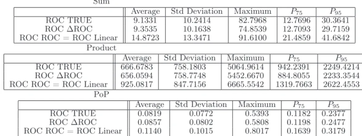
4.1.1 No information available about the reservation levels of the parties

In Table 1 it is possible to see the value loss of the different rules considering the different criteria, i.e., the difference between the real value of the real best alternative and the real value of the alternative chosen by the rule. This table shows the average, the standard deviation, the maximum, the 75th percentile and the 95th percentile of the value loss. As expected, the worst results are obtained using ROC ROC / ROC Linear (because these are the cases in which less information is required from negotiators). Using ROC TRUE or ROC ∆ROC the results are very similar. The value loss is not very high even considering ROC ROC / ROC Linear.

Table 2 presents the proportion of cases in which the chosen alternative is efficient (using the different rules and considering the different criteria). Using the ROC TRUE the proportion is highest and using the ROC ROC / ROC Linear the proportion is lowest (as expected). In the cases in which the chosen alternative is not efficient it is interesting to know the distance to the nearest efficient alternative. The results are presented in Tables 3 and 4, using the L2 and L∞ distances, respectively. In these tables it

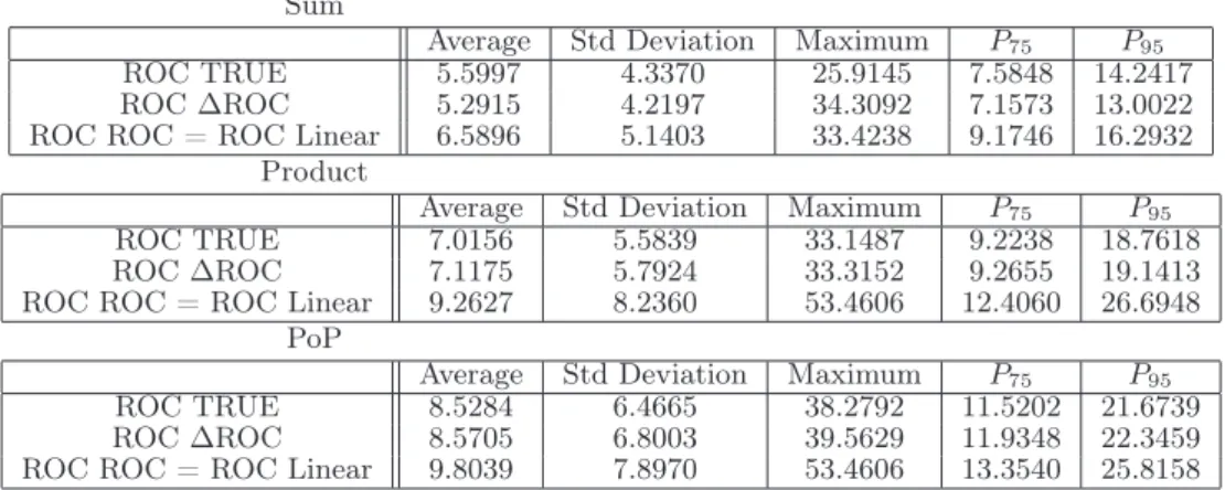
is possible to see the average, the standard deviation, the maximum, the 75th percentile and the 95th percentile of the distance. Considering the Euclidean distance, the best results (lower distances) are obtained using the ROC TRUE and ROC ∆ROC (these rules presented very similar results). Using the other distance (L∞), the conclusions are the same. Note that the different rules yield worse results for

the criterion of maximizing the minimal PoP than the other criteria. The proportion of cases in which the chosen alternative is efficient is not very high and, besides that, when the chosen alternative is not efficient the distance to the closest efficient alternative is not so small.

(10)

We computed some statistics tests to check if the difference between the ROC TRUE and ROC ∆ROC rules is significative (these are the two rules that provide the best results). We determined the p - value, i.e., the lowest level of significance at which the hypothesis of equality of the rules can be rejected. The results are presented in Table 5. In this table it is possible to see the p - value when comparing the average of the value loss, the average of the Euclidean distance, the average of the L∞ distance of the

two rules and also the proportion of cases in which the chosen alternative is efficient. As it is possible to see considering the proportion of cases in which the chosen alternative is efficient, and using the criterion maximizing the sum of the values, the ROC TRUE rule is better. In all the other cases the difference between the two rules is not significative. It seems that the ROC ROC rule is the one which provide worst results. We also computed some statistics tests to check if the difference between the ROC ROC and ROC ∆ROC rules are significative. As the p-values are equal to zero or very close, we can conclude that the ROC ∆ROC rule is better than the ROC ROC rule.

We can see in Tables 6 and 7 the difference between the real value of the best alternative and the real value of the alternative chosen by the used criteria, for Nelson and Amstore, respectively. In these tables it is possible to see the average of the difference. As it is possible to see, the best approximation for Nelson would occur if maximizing the minimal PoP was used, because the average difference is small. Even using this criterion, in average, Nelson loses with respect to the real best alternative, because the difference is positive. When maximizing the sum of the values, worse approximations for Nelson appear. The best results (smaller differences) are obtained using the ROC TRUE rule and the worst (bigger differences) are obtained using ROC ROC / ROC Linear rule. Using the the sum of the values criterion, in average, Amstore wins comparing with the real best alternative. For Amstore, the least favorable approximations are obtained using the criterion maximizing the minimal PoP. It is possible to see that, in average, both parties lose in using the rules instead of real values, except Amstore with the criterion maximizing the sum of the values. It is possible to consider that the criterion maximizing the minimal PoP provides a fair (unbiased) approximation, because the considered difference is similar for both parties. The same does not happen for the criterion maximizing the sum of the values.

Detailed results related to the position that the best alternative according to the different rules reached in the supposedly true ranking, are presented in Table 8. This table shows, for each rule and for each criteria, the average position on the supposedly true ranking (the minimum position was always 1) and the proportion of cases where the position reached is 1, ≤ 2, ≤ 3, ≤ 4, ≤ 5, ≤ 10 and ≤ 20. This table gives us the information to know how many alternatives should be chosen to guarantee the retention of the supposed best alternative. As expected, as the total number of alternatives is equal to 70, retaining only one alternative is not sufficient in the majority of the cases. However, even then, we can consider that the “hit rate”, i.e., the proportion of cases in which the best alternatives in the two rankings coincide, is not very bad. Retaining 20 alternatives (close to 30% of the total number of alternatives) the probability of retaining the best one is almost always higher than 90%. The hit rate using the ROC ROC / ROC Linear values and the criterion maximizing the sum of the values is surprisingly high. This happens because the high number of ties (using ROC / Linear values, the value functions of both parties are symmetrical, and because of that, when the weights match there are a lot of alternatives with equal sum of values).

Results relatively to the position of the best alternative using the different rules in the supposedly true ranking are shown in Table 9. These results enable us to know how good is the alternative chosen by each rule in terms of the supposedly true ranking. Note that the value of the hit rate should be the same considering the position of the supposedly best alternative in the rankings induced by the rules and the position of the best alternative using the different rules in the supposedly true ranking. However this did not happen because, if there are ties in the first place of the ranking, which is frequent when the different rules are used, the chosen alternative is the first one with position in the ranking equal to one. Because of that, the hit rate considering the position of the supposedly best alternative in the ranking induced by the different rules is superior or equal than the hit rate considering the position of the best alternative using the different rules in the supposedly true ranking. These results complement the ones regarding the value loss, the proportion of cases in which the chosen alternative is efficient and, if the alternative is not efficient, the distance to the nearest efficient alternative. In more than 81% of the cases the alternative chosen by the rule is one of the best 20 ones. If we consider the ROC TRUE and ROC ∆ROC rules, in more than 83% of the cases the alternative chosen by the rule is one of the best 10 ones.

(11)

4.1.2 Information available about the reservation levels of the parties

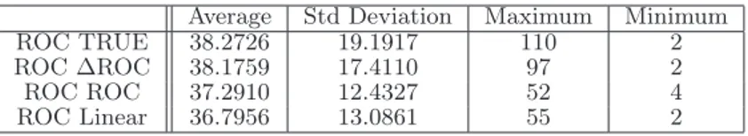
In this section we considered that an alternative needs to be better than the reservation levels, for both parties, to be admissible. In our simulation study, there were cases in which there was no alternative better than the reservation levels for both parties. We eliminated these cases and increased the number of simulations in such a way to have 5000 valid examples. In Table 10 it is possible to see the average, the standard deviation and maximum number of alternatives better for both parties than the reservation levels (the minimum number was always equal to 1). Note that, using all the rules, the average number of alternatives better than the reservation levels is near 19 alternatives (in a total of 70 alternatives). In the original problem we have 26 alternatives better than the reservation levels for both parties. To determine a realistic value loss we decided to analyze only the cases in which the alternative provided by each rule is admissible. Indeed, no value loss would occur if the alternative proposed by the mediator was unacceptable for one of the parties, since there would be no agreement. As a curiosity, in Table 11 we present the proportion of cases in which each rule provides a non admissible alternative.

Table 12 presents the value loss of the different rules considering the different criteria. As expected, the worst results are obtained using ROC ROC / ROC Linear rule. Comparing with the results considering no reservation levels it is possible to see that the value loss of the criterion maximizing the sum of the values is slightly lower and the value loss of the criterion maximizing the minimal PoP is slightly higher in this case. These results are normal since we are excluding of the analysis some alternatives (the non admissible ones). Using the criterion maximizing the product of the excesses the value loss is much higher considering no reservation levels because in this case the aggregated global value is also much higher.

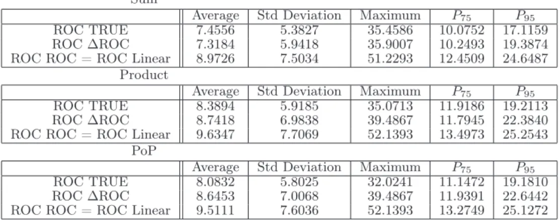
In Table 13, it is possible to see the proportion of cases in which the chosen alternative is efficient. Using the ROC TRUE rule the proportion is highest and using the ROC ROC / ROC Linear rule the proportion is lowest. With the criterion maximizing the minimal PoP, using the three rules, the proportion of cases in which the chosen alternative is efficient is higher considering information regarding the reservation levels. The opposite happens considering the criterion maximizing the sum of the values. In the cases in which the chosen alternative is not efficient we determined the distance to the nearest efficient alternative. The results are presented in Tables 14 and 15, using the L2 and L∞ distances,

respectively. Considering the Euclidean distance, the best results are obtained using the ROC TRUE rule. Using the criterion maximizing the sum of the value, with all the rules, the results are better considering no reservation levels. The opposite happens when it is use the criterion maximizing de minimal PoP. With the L∞ distance the conclusions are the same.

We computed some statistics tests to check if the difference between the ROC TRUE and ROC ∆ROC rules are significative. The obtained p-values are presented in Table 16. As it is possible to see the difference between the two rules is significative considering the value loss and the criterion maximizing the minimal PoP, considering the proportion of cases in which the chosen alternative is efficient and using the criteria maximizing the sum of the values and maximizing the product of the excesses regarding the reservation level. In these cases the ROC TRUE rule presents better results. Remember that considering no reservation levels the difference between the two rules is only significative considering the proportion of cases in which the chosen alternative is efficient and using the criterion maximizing the sum of the values. It seems that the ROC ROC / ROC Linear rule is the one which provides worst results. Table 17 presents the p-values obtained when the objective was to check if the difference between the ROC ∆ROC and ROC ROC / ROC Linear rules is significative. Considering the distances and the criteria maximizing the minimal PoP and maximizing the product of the excesses it is not possible to consider that the ROC ∆ ROC rule is better. Remember that considering no reservation levels it is possible to conclude that the ROC ∆ ROC rule is always better.

We also computed some statistics tests to compare the ROC ∆ROC rule considering no reservation levels and considering reservation levels. Results are presented in Table 18. We chose this rule because between the two best rules is the one which require less information from negotiators. The difference between the two cases is significative considering the value loss and the criterion maximizing the product of the excesses, considering the proportion of cases in which the chosen alternative is efficient and the criterion maximizing the minimal PoP, and considering the L∞distance and the criterion maximizing the

minimal PoP. In these cases better results are obtained considering reservation levels. Considering the value loss and the criterion maximizing the minimal PoP, and the distances and the criterion maximizing the sum of the values, the best results are obtained considering no reservation levels.

(12)

Tables 19 and 20 show the difference between the value of the best alternative and the value of the alternative chosen by the used criteria, for Nelson and Amstore, respectively. As it is possible to see, the rules are less prejudicial for Nelson when maximizing the product of the excesses regarding the reservation levels. Even using this criterion, in average, Nelson loses with respect to the real best alternative. The best results are obtained using the ROC TRUE rule and the worst are obtained using ROC ROC / ROC Linear rule. For Amstore, the criterion for which rules are more beneficial is to maximize the sum of the values. With this criterion, in average, Amstore wins comparing with the real best alternative. It is possible to see that, in average, both parties lose in using the rules instead of real values, except Amstore with the criterion maximizing the sum of the values. Note that considering no reservation levels the worst/best criterion for Nelson/Amstore was the same (maximizing the sum of the values) the same does not happen to the best/worst criterion for Nelson/Amstore. With these results it is also possible to consider that when the criterion maximizing the sum of the values is used, the rules does not provide a fair approximation (as it was concluded considering no reservation levels).

Results related to the position that the best alternative according to the different rules reached in the supposedly true ranking, are presented in Table 21. This table gives us the information to know how many alternatives should be chosen to guaranty the retention of the supposed best alternative. Retaining 20 alternatives the probability of retaining the best is always higher than 90%. The differences between the results considering no reservation levels and considering reservation levels are not very significative. Results relatively to the position of the best alternative using the different rules in the supposedly true ranking are shown in Table 22. In more than 90% of the cases the alternative chosen by the rule is one of the best 20 ones. If we consider the ROC TRUE and ROC ∆ROC rules, in more than 85% of the cases the alternative chosen by the rule is one of the best 10 ones. The results are slightly better than the results obtained considering no reservation levels.

4.2 Examples based on the Itex vs Cypress template

4.2.1 No information available about the reservation levels of the parties

Tables 23 and 24 show the value loss of the different rules and the proportion of cases in which the chosen alternative is efficient, respectively. In the cases in which the chosen alternative is not efficient we determined the distance to the nearest efficient alternative. The results are presented in Tables 25 and 26, using the L2and L∞distances, respectively.

As it is possible to see the ROC ROC and ROC Linear rules are the ones which provide worst results, and ROC TRUE and ROC ∆ROC rules are the ones which provide best results. We computed some statistics tests to check if the difference between the ROC TRUE and ROC ∆ROC rules are significative. The results of the p-values are presented in Table 27. It is possible to see that the difference between the two rules is significative considering the value loss and considering the proportion of cases in which the chosen alternative is efficient. In these cases the ROC TRUE rule present better results. Note that in this example the difference between the two rules is more significative than in the example presented in section 4.1.1. The results of the statistics tests comparing the ROC ROC and ROC Linear rules are presented in Table 28. Observing the p-values it is possible to conclude that the difference between the two rules are not significative. We also compared the ROC ∆ROC and ROC ROC rules (one of the best and one of the worst) to check if the difference between them are significative. In all the cases we obtained p-values equal to zero, what means that the difference between the rules is significative. So, it is possible to conclude that the ROC ∆ROC rule presents better results than the ROC ROC rule. Note that, in section 4.1.1 we concluded the same.

In Tables 29 and 30, we can see the difference between the value of the best alternative and the value of the alternative chosen by the used criteria, for Itex and Cypress, respectively. As it is possible to see, the best approximation for Itex occurs when maximizing the minimal PoP, because the average difference is small. Even using this criterion, in average, Itex loses with respect to the real best alternative, because the difference is positive. The worst criterion for Itex is maximizing the sum of the values. For Cypress, the best criterion is to maximize the sum of the values but, even with this criterion, in average, Cypress loses comparing with the real best alternative. For Cypress, the worst results are obtained using the criterion maximizing the product of the excesses regarding the reservation levels. It is possible to see that, in average, both parties loses in using the rules instead of real values. With these results it is also possible to see if the alternative chosen by the rule is a fair approximation. As we concluded in subsection

(13)

4.1.1., it is possible to consider that using the criterion maximizing the sum of the values, the rules do not provide a fair approximation.

Results related to the position that the best alternative according to the different rules reached in the supposedly true ranking, are presented in Table 31. As expected, as the total number of alternatives is equal to 180, retaining only one alternative is not sufficient in the majority of the cases. However, even then, we can consider that the hit rate, is quite reasonable. Retaining 20 alternatives (close to 12% of the total number of alternatives) the probability of retaining the best is higher than 85%, considering the ROC TRUE and ROC ∆ROC rules. Retaining 20 alternatives in this example correspond, more or less, to retaining 10 alternatives in the example presented in the last section. The obtained results are not very different. Results relatively to the position of the best alternative using the different rule in the supposedly true ranking are shown in Table 32. In more than 72% of the cases the alternative chosen by the rule is one of the best 20 ones. If we consider the ROC TRUE and ROC ∆ROC rules, in more than 74% of the cases the alternative chosen by the rule is one of the best 10 ones. Once more, the obtained results are not very different from the ones obtained in subsection 4.1.1.

4.2.2 Information available about the reservation levels of the parties

In Table 33, it is possible to see the average, the standard deviation and maximum number of alternatives better than the reservation levels for both parties, considering that the reservation level of Itex is equal to VI_(x

86) and the reservation level of Cypress is equal to VC(x95). Note that, using all the rules, the

average number of alternatives better than the reservation levels is near 38 alternatives (in a total of 180 alternatives). We will not present the results obtained considering that the reservation levels are equal to the values of the alternatives 52 and 129, for Itex and Cypress, respectively, because they are not very different from the ones obtained considering that there are no reservation levels.

We can see in Table 34 the proportion of cases in each the alternative chosen by each rule is not admissible. Table 35 shows the value loss of the different rules considering the different criteria and Table 36 shows the proportion of cases in which the chosen alternative is efficient. In the cases in which the chosen alternative is not efficient we determined the distance to the nearest efficient alternative. The results are presented in Tables 37 and 38, using the L2 and L∞ distances, respectively.

We performed some statistical tests to check if the difference between the ROC TRUE values and ROC ∆ROC rules (the two best rules) are significative. The results of the p-values are presented in Table 39. The only cases where it is not possible to conclude that the ROC TRUE rule is better is considering the distances and the criterion maximizing the product of the excesses regarding the reservation levels. Note that the difference between the two rules is more significative considering reservation levels and more significative than in section 4.1.2. The ROC ROC and ROC Linear rules are the ones which provide worst results, so we computed some statistics tests to see if the difference between them is significative. The results are presented in Table 40. In all the cases it is possible to conclude that the two rules present similar results (as it was concluded considering no reservation levels). Similarly to what we done in the previous subsection we also compared the ROC ∆ROC and ROC ROC rules. In all the cases we obtained p-values equal to zero, or very close, what means that the difference between the two rules is significative, this difference is favorable to the ROC ∆ROC rule. This is the same conclusion we obtained considering no reservation levels. Remember that in the examples for the Nelson vs. Amstore template (see section 4.1.2) it was not always possible to conclude that the ROC ∆ROC rule is better.

As in the examples for the Nelson vs. Amstore template, we compared the ROC ∆ROC rule consid-ering reservation values and considconsid-ering no reservation levels (see results in Table 41). Considconsid-ering the value loss and the criteria maximizing the sum of the values and maximizing the product of the excesses the best results are obtained considering reservation levels. Considering the value loss and the criterion maximizing the minimal PoP, the proportion of cases in which the chosen alternative is efficient and the criteria maximizing the sum of the values and maximizing the minimal PoP, the distances and the criterion maximizing the product of the excesses the best results are obtained considering no reservation levels. The results are very different from the ones obtained in subsection 4.1.2. However this difference is natural since in one example we are considering reservation levels very different between the parties and in the other example the reservation levels of both parties are similar.

In Tables 42 and 43, it is possible to see the difference between the value of the best alternative and the value of the alternative chosen by the used criteria, for Itex and Cypress, respectively. The rules

(14)

provide a better approximation for Itex when maximizing the minimal PoP. Even using this criterion, in average, Itex loses with respect to the real best alternative. For Cypress, the best approximation occurs for the criterion maximize the sum of the values but even with this criterion, in average, Cypress loses comparing with the real best alternative. The conclusions are the same obtained considering no reservation levels.

Table 44 presents the position that the best alternative according to the different rules reached in the supposedly true ranking. Results relatively to the position of the best alternative using the different rule in the supposedly true ranking are shown in Table 45. The results are not very different from the ones considering no reservation levels.

5 Conclusions

In bilateral Negotiation Analysis, the literature often considers the case with complete information, which cannot be applied in practice when the parties do not have complete information. In this work we considered a setting of bilateral integrative negotiation over multiple issues in which the preferences of both parties can be roughly modelled by an additive value function. We compared four decision rules (ROC TRUE, ROC ∆ROC, ROC ROC and ROC Linear) to help a mediator suggesting an alternative under these circumstances, considering that there exists ordinal information both on the scaling weights and on the level’ values, and tested them using Monte-Carlo simulation.

We compared the four rules using two cases as templates for generating random examples (one with 70 alternatives and the other one with 180 alternatives). In all cases we used three criteria: maximizing the sum of the values, maximizing the product of the excesses regarding the reservation levels and maximizing the minimal PoP. Note however that our objective was not to compare the criteria but to compare the rules. The choice of the used criteria depends on the mediator preferences.

To compare the rules we determined the proportion of cases in which each rule chose the really best alternatives and in the cases in which the two rules did not match we determined the value loss. We determined the proportion of cases in which the alternative chosen by each rule is efficient, and for the inefficient ones we determined the distance to the nearest efficient alternative (using the L2 and L∞

distances). The results using the two cases as templates for generating random examples were different and the results considering no reservation levels and considering reservation levels were also different. But, it is possible to conclude that the best results were obtained using the ROC TRUE and ROC ∆ROC rules. There are cases in which it is possible to consider that these rules are equivalent which is, in a certain way, surprising, because in the ROC TRUE rule we require cardinal information about the levels’ values from the negotiators. The ROC ROC and ROC Linear rules are the worst ones, and it is possible to consider that the difference between them is not significative. The ROC ∆ROC rule is, almost always, better than the ROC ROC rule. We determined also the difference between the real value of the best alternative and the real value of the alternative chosen by the used criterion, for both parties. This enables us to know whether using only ordinal information leads to treat one of the parties unfairly, when compared to a situation in which precise cardinal values were used instead. We also compared the ranking of the alternatives according to the supposedly true parameters with the ranking of the alternatives according to the used decision rule, we considered the following results: the position that the best alternative according to the true ranking reaches in the ranking generated by the used decision rule (this allows us to know the minimum number of alternatives that must be chosen, beginning by the top of the ranking provided by the rule, so that the true best alternative belongs to the chosen set) and the position that the best alternative in the ranking generated by the rule reaches in the supposedly true ranking (this allows us to know how good the alternative chosen by the rule is in terms of the supposed true ranking).

In our opinion the results are encouraging. Considering that the total number of alternatives is high the hit rate is relatively good and when the rule does not choose the real true alternative the average value loss is not very high. The proportion of cases in which the chosen alternative is efficient is high and when the chosen alternative is not efficient the distance to the nearest efficient alternative is not very high. The position that the best alternative in the ranking generated by the rule reaches in the supposedly true ranking complements that results that show the alternative chosen by the rule is typically a good alternative. In the majority of the cases negotiators, in average, lose in using the rules instead of real values for all the criteria, however the average loss is not very high. The criterion maximizing the

(15)

sum of the values is the one which provides less balanced approximations between the two parties. It was possible to see that, although the hit rate is relatively high, retaining one alternative is not sufficient in the majority of the cases. But, if instead of one alternative, the mediator keeps for example a set of 20 alternatives, the probability of this set containing the real best alternative is very high. The position that the best alternative according to the true ranking reaches in the ranking generated by the used decision rule allowed us to assess the strategy of retaining k < m alternatives instead of only one.

Acknowledgements:

This work benefited from support of FCT/FEDER grant POCI/EGE/58371/2004.

References

[1] Ahn, B.S. and Park, K.S. (2008), Comparing methods for multiattribute decision making with ordinal weights, Computers & Operations Research 35, pp. 1660-1670.

[2] Barron, F.H. and Barret, B.E. (1996), Decision Quality Using Ranked Attribute Weights, Manage-ment Science 42 (11), pp. 1515-1523.

[3] Butler, J., Jia, J. and Dyer, J. (1997), Simulation Tecniques for the Sensitivity Analysis of Multi-criteria Decision Models, European Journal of Operational Research 103, pp. 531-546.

[4] Clímaco, J. and Dias, L.C. (2006), An Approach to Support Negotiation Processes With Imprecise Information Multicriteria Additive Models, Group Decision and Negotiation 15 (2), pp. 171-184.

[5] Ehtamo, H., Hämäläinen, R.P., Heiskanen, P., Teich, J., Verkama, M. and Zionts, S. (1999), Gen-erating Pareto solutions in a two party setting: Constraint proposal methods, Management Science 45 (12), pp. 1697-1709.

[6] Heikanen, P. (1999), Decentralized method for computing Pareto solutions in multiparty negotiation, European Journal of Operational Research 117, pp. 578-590.

[7] Jelassi, T., Kersten, G. and Zionts, S. (1998), An Introduction to Group Decision and Negotiation Support, in Bana e Costa (eds.), Readings in Multiple Criteria Decision Aid, Springer-Verlag, Berlin, 537-568.

[8] Keeney, R.L. and Raiffa, H. (1976), Decisions with Multiple Objectives: Preferences and Value Tradeoff, John Wiley and Sons, New York. (more recent version publicated in 1993 by Cambridge University Press)

[9] Kersten, G.E. and Noronha, S.J. (1998), Negotiation and the Internet: Users’ Expectations and Acceptance, INR01/98

[10] Lahdelma, R., Miettinen, K. and Salminen, P. (2003), Ordinal Criteria in Stochastic Multicriteria Acceptability Analysis (SMAA), European Journal of Operational Research 147, pp. 117-127.

[11] Lai, G., Li, C. and Sycara, K. (2006), Efficient Multi-Attribute Negotiation with Incomplete Infor-mation, Goup Decicion and Negotiation 15, pp. 511-528.

[12] Raiffa, H. with J. Richardson and D. Metcalfe (2002), Negotiation analyis: the science and art of collaborative decision making, Cambridge (Ma), Belknap Press of Harvard, University Press.

[13] Roy, B. and Mousseau, V. (1996), A theoretical framework for analysing the notion of relative importance of criteria, Journal of Multi Criteria Decision Analysis 5, pp. 145-159.

[14] Salo, A.A. and Hämäläinen, R.P. (2001), Preference Ratios in Multiatribute Evaluation (PRIME) -Elicitation and Decision Procedures Under Incomplete Information, IEEE Transactions on Systems, Man, and Cybernetics, Part A 31 (6), pp. 533-545.

(16)

[15] Salo, A. and Punkka, A. (2005), Rank Inclusion in Criteria Hierarchies, European Journal of Oper-ational Research 163 (2), pp. 338-356.

[16] Sarabando, P. and Dias, L.C. (in print), Multi-attribute choice with ordinal information: a compar-ison of different decision rules, IEEE Transactions on Systems, Man, and Cybernetics, Part A, to appear.

[17] Sarabando, P. and Dias, L.C. (2009), Simple procedures of choice in multicriteria problems without precise information about the alternatives’ values, Research Reports of INESC Coimbra, No. 1/2009.

[18] Stewart, T.J. (1995), Simplified approaches for multicriteria decision making under uncertainty, Journal of Multi-Criteria Decision Analysis 4, 246-258.

[19] Vetschera, R. (2008), Learning about prefereneces in electronic negotiations - a volume based mea-surement method. European Journal of Operational Research, page in print.

[20] Weber, M. (1987), Decision making with incomplete information, European Journal of Operational Research 28, pp. 44-57.

[21] Winterfeldt, D.V. and Edwards, W. (1986), Decision Analysis and Behavioral Research, Cambridge University Press, New York.

(17)

A

Results

Sum

Average Std Deviation Maximum P75 P95

ROC TRUE 9.1331 10.2414 82.7968 12.7696 30.3641

ROC ∆ROC 9.3535 10.1638 74.8539 12.7093 29.7159

ROC ROC = ROC Linear 14.8723 13.3471 91.6100 21.4859 41.6842 Product

ROC TRUE 666.6783 758.1803 5064.9614 942.2391 2249.4214

ROC ∆ROC 656.0594 758.7748 5452.6670 884.8055 2233.3544

ROC ROC = ROC Linear 925.0817 847.7156 6665.5542 1319.7663 2622.4553 PoP

ROC TRUE 0.0819 0.0772 0.5393 0.1182 0.2377

ROC ∆ROC 0.0857 0.0802 0.5808 0.1198 0.2477

ROC ROC = ROC Linear 0.1140 0.1015 0.8017 0.1639 0.3179

Table 1: Value Loss (reservation levels equal to 0 for Nelson and Amstore). Sum Product PoP

ROC TRUE 94.26 91.06 80.92

ROC ∆ROC 92.22 90.22 79.18

ROC ROC = ROC Linear 88.72 78.36 67.46

Table 2: Proportion of cases in which the chosen alternative is efficient (reservation levels equal to 0 for Nelson and Amstore).

Sum

ROC TRUE 6.3796 4.9173 26.3772 8.5454 15.9898

ROC ∆ROC 6.0499 4.8757 38.7505 8.1107 15.4725

ROC TRUE 7.9482 6.2996 42.2776 10.1963 21.1535

ROC ∆ROC 8.0421 6.4076 36.5928 10.5669 20.9423

ROC TRUE 9.5344 7.1672 42.0696 12.6078 24.4005

ROC ∆ROC 9.5435 7.4248 42.6280 13.1596 24.7427

Table 3: Distance between the chosen alternative and the nearest efficient alternative - Euclidean distance (reservation levels equal to 0 for Nelson and Amstore).

(18)

Sum

ROC TRUE 5.5997 4.3370 25.9145 7.5848 14.2417

ROC ∆ROC 5.2915 4.2197 34.3092 7.1573 13.0022

ROC TRUE 7.0156 5.5839 33.1487 9.2238 18.7618

ROC ∆ROC 7.1175 5.7924 33.3152 9.2655 19.1413

ROC TRUE 8.5284 6.4665 38.2792 11.5202 21.6739

ROC ∆ROC 8.5705 6.8003 39.5629 11.9348 22.3459

Table 4: Distance between the chosen alternative and the nearest efficient alternative - L∞ distance (reservation levels equal to 0 for Nelson and Amstore).

Sum Product PoP

Value Loss 0.4037 0.5889 0.0390 Efficient 0.0001 0.1493 0.0294 Euclidean Distance 0.3872 0.8213 0.9778

L∞Distance 0.3556 0.7841 0.8873

Table 5: p - values comparing the ROC TRUE and ROC ∆ROC rules (reservation levels equal to 0 for Nelson and Amstore).

Sum Product PoP

ROC TRUE 8.3781 3.4446 3.2014

ROC ∆ROC 8.8379 4.0453 3.4283

Table 6: Average of the difference between the value of the best alternative and the value of the alternative chosen by the used criterion, for Nelson (reservation levels equal to 0 for Nelson and Amstore).

Sum Product PoP

ROC TRUE -3.1522 1.8095 3.2114

ROC ∆ROC -2.9489 1.8195 2.8835

ROC ROC = ROC Linear -9.4563 5.0615 5.9737

Table 7: Average of the difference between the value of the best alternative and the value of the alternative chosen by the used criterion, for Amstore (reservation levels equal to 0 for Nelson and Amstore).

(19)

Sum