Modelling rodent distribution in Índia, with special reference to wildcats prey

2015

UNIVERSIDADE DE LISBOA FACULDADE DE CIÊNCIAS DEPARTAMENTO DE BIOLOGIA ANIMAL

Modelling rodent distribution in India, with special reference to

wildcats prey

Mestrado em Biologia da Conservação

Filipa Leça Pereira Gouveia Marques

Dissertação orientada por:

Prof.ª Doutora Margarida dos Santos Reis Doutor Luís Miguel Rosalino

i AGRADECIMENTOS

Gostaria de começar por agradecer aos meus orientadores, Profª Dra. Margarida dos Santos Reis e Dr. Luís Miguel Rosalino, em especial ao Miguel por toda a ajuda e apoio que me deu ao longo da escrita desta tese, que se acabou por revelar mais complicada e trabalhosa do que inicialmente esperado.

Um obrigado especial ao meu orientador externo André, por toda a ajuda e paciência que demonstrou durante todo este longo percurso.

Não podia deixar de agradecer também a todos meus colegas de mestrado mas em especial ao Ricardo e à Catarina, por toda a companhia que me fazem, pelas palavras de encorajamento e pelas informações cruciais à entrega desta tese!

Aos meus pais, por terem lido a tese e ajudado com as suas opiniões e ideias, e por fim, um obrigado muito especial ao meu marido João cuja ajuda, amizade, carinho e, acima de tudo, paciência, foram indispensáveis.

RESUMO

O subcontinente Indiano é considerado um “hotspot” de biodiversidade e, por isso, tem sido alvo de vários estudos de conservação, particularmente centrados no impacto do crescimento e desenvolvimento industrial da população humana na vida selvagem. A grande parte destes estudos foca-se em mamíferos, nomeadamente em espécies carismáticas como o tigre ou o elefante asiático, havendo poucos projetos centrados na conservação das espécies pertencentes a níveis mais baixos da cadeia trófica, como os roedores, que, no entanto, influenciam os restantes componentes dos ecossistemas devido a efeitos em cascata (ex. dispersão de sementes, predação).

Esta tese de mestrado é parte integrante de um estudo mais alargado que pretende avaliar a importância presente e futura das áreas protegidas para pequenos felinos, tendo em conta diferentes cenários climáticos no subcontinente Indiano. O objetivo principal deste trabalho é a avaliação dos padrões de distribuição de roedores, particularmente as espécies-presa de pequenos felinos, utilizando uma aproximação macroecológica como método de avaliação primário dos requisitos ecológicos destes animais.

Foram recolhidos de diferentes bases de dados, informações de presença de roedores previamente identificados como presas de pequenos felinos. Estes foram primariamente divididos em 3 grupos de acordo com o seu peso médio descrito (até 70g – “Pequeno”; entre 70g e 150g – “Médio”, acima de 150g – “Grande”), representando diferentes importâncias energéticas para os felinos. Os dados foram também agrupados num único grupo denominado “Total”. Com base na distribuição espacial destes dados, estimou-se a probabilidade de presença de cada grupo e dos roedores em geral no subcontinente Indiano, baseada em variáveis bioclimáticas, de cobertura do solo, altitude e densidade populacional humana, através de um modelo de distribuição de espécies de máxima entropia (Maxent).

Para a categoria “Pequeno”, obteve-se um modelo Maxent com AUC = 0.753, cujas variáveis que parecem ter maior influência na ocorrência das espécies deste grupo são a cobertura do solo (25.2% de contribuição para o modelo gerado, onde a classe de maior importância é “aldeamentos”, relacionada com uma probabilidade de presença de roedores acima de 0.9), a precipitação do trimestre mais seco (Bio17: 22.1%), sazonalidade da

iii do trimestre mais frio (Bio19: 11.2%). Tal como no modelo acima referido, o modelo para “Médio”, com AUC = 0.752, tem como variável mais importante a cobertura do solo (30.6%), cuja classe mais importante é também “aldeamentos” (com uma probabilidade associada de ocorrência de roedores acima dos 0.9). As outras variáveis de maior importância no modelo gerado são a sazonalidade da temperatura (Bio4: 22.1%) e a precipitação do trimestre mais frio (Bio19: 16.7%), não havendo mais variáveis com percentagens de contribuição para o modelo acima de 10%. O modelo gerado para o grupo “Grande” é o que mais difere quando comparado com todos os modelos gerados, sendo também o modelo com maior valor de AUC (AUC = 0.774). Tal como nos outros modelos gerados, a variável mais importante no modelo continua a ser a cobertura do solo (27.9%), e a classe mais relevante dentro desta variável é “aldeamentos”, com uma probabilidade de ocorrência de roedores associada de 0.9. Para este modelo, as outras variáveis mais importantes são a densidade populacional (19.2%), a altitude (15.3%) e a sazonalidade de temperatura (Bio4: 14.1%). Finalmente, o modelo gerado para “Total” tem um valor de AUC = 0.74, aparecendo de novo a cobertura do solo como a variável mais importante (31.4%, “aldeamentos” com probabilidade de ocorrência de roedores de 0.9), seguida pela sazonalidade da temperatura (Bio4: 22.3%), a precipitação do trimestre mais frio (Bio19: 11.6%) e por fim a precipitação do trimestre mais seco (Bio17: 11.5%).

O modo como cada uma das variáveis tidas como importantes aos modelos gerados influencia a probabilidade de ocorrência de roedores não varia substancialmente entre os modelos. Áreas onde sazonalidade da temperatura (Bio4) é menor aparentam ter uma maior probabilidade de ocorrência de roedores associada (esta variável é, portanto, inversamente proporcional à probabilidade de ocorrência de roedores). A curva de resposta da probabilidade de ocorrência relativamente à precipitação do trimestre mais frio (Bio19) mostra que a probabilidade de ocorrência de roedores aumenta em áreas cuja precipitação neste trimestre é moderada, mas diminui para áreas onde chove muito durante esta estação, que tende a ser a mais fria e seca do ano. Ainda relativamente à precipitação, desta vez do trimestre mais seco (Bio17), as curvas de resposta dos modelos onde esta variável aparece como importante mostram que áreas onde chove mais durante esta estação estão associadas a uma maior probabilidade de ocorrência de roedores. Por fim, tendo em vista as variáveis que apareceram exclusivamente como mais importantes para o modelo Maxent gerado para

o grupo “Grande”, a probabilidade de ocorrência de roedores parece aumentar de forma logarítmica relativamente à densidade populacional, atingindo valores próximos de 1.0 a partir das 5000 pessoas por Km2, mostrando que em áreas com maior densidade populacional, a probabilidade de ocorrência de roedores deste grupo é quase certa. Já a altitude parece não ter grande influência na probabilidade de ocorrência de roedores de maior tamanho até aos 2500m de altitude (metros acima do nível do mar), sendo que a partir deste valor desce drasticamente, mostrando que em áreas mais elevadas (como regiões montanhosas) a probabilidade de ocorrência de roedores de maior tamanho é muito baixa.

As análises dos modelos Maxent obtidos revelaram que existe uma forte relação entre a distribuição de roedores e a presença do Homem (associação da ocorrência de roedores acima dos 90% em áreas correspondentes a “aldeamentos”), assim como uma ligação entre a distribuição destas espécies com condições climáticas mais moderadas, onde existe menor variação de temperatura ao longo do ano, assim como alguma precipitação durante a estação mais fria e seca.

A associação entre uma maior ocorrência de roedores e zonas com maior densidade populacional Humana poderá dever-se não só à maior facilidade de encontrar alimento e abrigo, mas também à proteção contra predadores de maiores dimensões (como os pequenos felinos) que podem evitar estas mesmas zonas de maior densidade Humana, devido ao maior risco de serem caçados nestas áreas. A aparente relação entre áreas cujo clima é mais constante ao longo do ano e uma maior presença de roedores poderá dever-se ao facto de áreas onde temperatura não varia tanto e a precipitação é moderada, estarem associadas a um menor gasto de energia por parte dos roedores. Áreas com demasiada chuva poderão dificultar a mobilidade e a procura de abrigo, enquanto áreas demasiado secas estarão associadas com uma menor disponibilidade de comida, sendo, portanto, preferível aos roedores áreas onde existe chuva moderada ao longo de todo o ano principalmente durante a estação mais seca.

Os resultados desta tese poderão contribuir para: 1) a conservação de espécies cuja dieta se baseie no consumo roedores, pois permite identificar áreas com maior disponibilidade de presas (i.e. maior riqueza específica de presas); e 2) a conservação dos

v Indiano, estão muito pouco estudados, pois identifica variáveis que parecem condicionar a presença destas espécies.

No futuro seria importante uma recolha mais exaustiva de dados de presenças de roedores, especialmente nas áreas identificadas como tendo uma maior probabilidade de ocorrência associada, assim como confirmar a ausência de algumas espécies de certas regiões (i.e. verdadeiras ausências), principalmente nas áreas identificadas como tendo menor probabilidade de ocorrência de roedores, pois permitirá a construção de modelos com elevado valor preditivo associado.

Palavras-Chave:

Subcontinente Indiano, Pequenos mamíferos, Padrão de distribuição, Pequenos felinos, Maxent

ABSTRACT

Being an important biodiversity hotspot, the Indian subcontinent has been the target of many conservation studies, especially concerning the impact of human population growth and development on wildlife. Mammals have often been the focus of such studies, particularly top predators (e.g. tiger) and other charismatic species (e.g. Asian elephant), with few projects looking into the conservation of species occupying lower levels of the trophic net, such as rodents, that influence all the communities by cascading effects.

This thesis is integrated on a wider study evaluating the current and future importance of protected areas for small felids under predicted climate scenarios for the whole Indian subcontinent. It specifically aims to assess rodents (identified as wildcats’ prey) distribution patterns on a macroecological scale, as a primary evaluation of these rodents’ needs.

Presence data of rodents identified as wildcat’s prey were collected from different databases, divided into strategic sets of data and analysed together with bioclimate, altitude, population density and land cover variables, through the use of a Maxent species distribution model, to access species probability of presence in the study area and variables influencing it. Rodents were divided into 3 weight classes (small, medium and large), based on species probable energetic importance to felids, and also assessed as a single “rodents’ total” group.

The analysis of the obtained Maxent models show a correlation between rodent’s distribution and Human presence, as well as a connection between rodent’s distribution and moderate weather conditions, namely places with less temperature seasonality and where the driest months have moderate rainfall.

The findings of this study may contribute to: 1) the conservation of wildcats and other carnivores whose diet is based on rodents, by identifying areas with the wider prey-species diversity, as well as 2) to the conservation of rodents themselves, who, despite being one of the most well represented mammal group in India, is also much understudied, by identifying variables constraining their presence.

Contents

CHAPTER 1 – Introduction ... 1

1.1 Wildcats Conservation and the Importance of Rodents ... 2

1.2 Rodents in India ... 4

1.3 Macroecology Approach ... 5

1.4 Study Aims ... 6

CHAPTER 2 – Study Area ... 7

2.1 Characterization of the Study Area ... 8

2.1.1 India ... 9 2.1.2 Pakistan ... 10 2.1.3 Bangladesh ... 10 2.1.4 Nepal ... 10 2.1.5 Bhutan ... 11 2.1.6 Sri Lanka ... 11

2.2 Climate Regions of the Study Area ... 11

CHAPTER 3 – Methods ... 15

3.1 Statistical Maxent Model ... 16

3.2 Species Selection, Data Collection and Processing ... 16

3.2.1 Presence data ... 17

3.2.2 Independent variables ... 19

3.2.3 Independent variables set ... 24

3.3 Statistical Analysis ... 25

3.3.1 Maxent input ... 25

CHAPTER 4 – Results ... 29

CHAPTER 5 – Discussion ... 43

CHAPTER 6 – Conclusions ... 49

6.1 Limitations of this Study ... 50

6.2 Final Conclusions and Future Work ... 51

REFERENCES ... 52

Due to its geographical position and climate, the Indian subcontinent (India, Pakistan, Bangladesh, Nepal, Bhutan and Sri Lanka), and especially the south Indian region, is of extreme importance for wildlife conservation, as it includes some of the richest biodiversity niches in the planet, with a huge variety of flora and fauna (e.g. Western Ghats/Sri Lanka), which is considered one of the world biodiversity hotspots (Myers, Mittermeier, Mittermeier, da Fonseca, & Kent, 2000). India alone is one of the richest areas in terms of mammal diversity, with more than 300 species and about 70 endemisms (Myers et al., 2000). Moreover, it has a wide variety of mammalian carnivores, with many species of mustelids, viverrids, canids, and felids, among others (Aroon, 2008; Grassman, Tewes, Silvy, & Kreetiyutanont, 2005; Home & Jhala, 2009; Jaeger, Haque, Sultana, & Bruggers, 2007; Khan, 2004; Majumder, Sankar, Qureshi, & Basu, 2011; Mukherjee, Goyal, Johnsingh, & Pitman, 2004; Myers et al., 2000; Rana, Smith, & Siddiqui, 2005; Shehzad et al., 2012), some of which are highly threatened (e.g., the Malabar Civet, Viverra civettina (Blyth, 1862), considered Critically Endangered; IUCN Red List 2015 (“The IUCN Red List of Threatened Species. Version 2015.2”)). As in many regions of the world, most conservation efforts in this region have been focused on large size and/or aesthetically pleasant species, such as the Indian Rhinoceros, Rhinoceros unicornis (Linnaeus, 1758) (Foose & Van Strien, 1997) or the Asian Elephant, Elephas maximus (Linnaeus, 1758) (Sukumar, 2006), with few projects looking into the distribution, ecology and conservation of species occupying lower levels of the trophic net, such as rodents, which may influence different communities through cascading effects.

1.1 W

C

I

R

India harbours 15 of the 36 world felid species and therefore plays a key role on the global conservation of this family. Owing to its rich biodiversity, growing population and industrial development, India is the target of many conservation studies, but there is a huge lack of information regarding the majority of small-medium sized feline species, as most studies are focused on big felids such as the Leopard Panthera pardus (Linnaeus, 1758) and the Tiger Panthera tigris (Linnaeus, 1758). In fact, small cats (i.e. all felids genera

3 represented in field studies worldwide (Grassman et al., 2005), and in India in particular, even though some of those small felids are vulnerable (e.g. rusty-spotted cat Prionailurus rubiginosus (I. Geoffroy Saint-Hilaire, 1831)) and endangered (e.g. fishing cat Prionailurus viverrinus (Bennett, 1833)) according with the IUCN Red List. Conservation strategies (e.g. protected areas and connectivity corridors) rely on detailed ecological information for the target species. Knowledge on the species distribution and macroecology is essential for considering broad-scale conservation strategies. Most of the available small felids studies are focused on species diet (Grassman et al., 2005; Khan, 2004; Majumder et al., 2011; Mukherjee et al., 2004; Shehzad et al., 2012; André P. Silva, Kilshaw, Johnson, Macdonald, & Rosalino, 2013) and the current existing information for small felids in India and worldwide show that small felid occurrence is in general associated with the occurrence of its prey (André P. Silva, Kilshaw, et al., 2013). Rodents form the bulk of the diet of several small wildcat species (Nowell & Jackson, 1996) and its occurrence may be a strong predictor of wildcat presence (André P. Silva, Kilshaw, et al., 2013; André P. Silva, Rosalino, et al., 2013). For example, according to Mukherjee et al. (2004), a single jungle cat Felis chaus (Schreber, 1777), consumes around 4 rodents every day and about half of those are Golunda ellioti (Gray, 1837). The leopard cat’s diet, Prionailurus bengalensis (Kerr, 1792), is also mainly composed of rodents, mostly murids (about 90%) (Rajaratnam, Sunquist, Rajaratnam, & Ambu, 2007a). In fact, there are many other small-felid species that presumably rely on rodents as a main food source, such as the rusty-spotted cat and the desert cat Felis silvestris ornata (Gray, 1830) (Mukherjee et al., 2004). Some studies suggest that several of these species consume the most abundant rodents throughout the year and in each location (Grassman et al., 2005).

Thus, information about rodents’ environmental requirements at broad-scale is therefore crucial for effective wildcat conservation actions, namely in a climate change context (Travis, 2003). Such information may help future understanding of how rodents, and consequently their predators, may be influenced by the predicted future climatic patterns (Torres, Pablo Jayat, & Pacheco, 2013). Additionally, assessing the relative importance of prey distribution, climate and land cover variables on wildcats’ distribution is currently not possible due to the lack of rodent’s occurrence estimations at broad-scale.

1.2 R

I

Rodentia is the richest order among mammals with more than 2050 recognized species, accounting for about 40 percent of living mammals worldwide and are naturally present in every continent, except Antarctica (Giovanni Amori & Gippoliti, 2001). In India, the most common rodents, such as Mus musculus (Linnaeus, 1758), Rattus norvegicus (Berkenhout, 1769), Rattus rattus (Linnaeus, 1758), Bandicota indica (Bechstein, 1800) (Molur et al., 2005), have grown in numbers and expanded their distribution ranges due to the continuously growing human population and land conversion into agriculture over the past decades (Mukherjee et al., 2004). However, there are also many threatened small-mammals species (rodents included), mostly menaced by habitat loss (Molur et al., 2005) and other harmful effects associated to human activities (e.g. poison use as pests control (Brakes & Smith, 2005)) (Giovanni Amori, Gippoliti, & Helgen, 2008).

Unfortunately, the number of studies in India focused on rodents is scarce (G Amori & Gippoliti, 2003; Giovanni Amori, Gippoliti, & Luiselli, 2011; Giovanni Amori & Gippoliti, 2001; Nameer, Molur, & Walker, 2001). Most available studies that deal with rodent biodiversity and ecology target the influence of those features upon anthropic activities and Human health (e.g., crop destruction, plague eradication and transmitted disease). The ones that do focus on rodents are scattered through different subjects (mostly carnivore diets) and spatial scales, which make it very difficult to use its information and compare data with ongoing studies.

A review of ecological studies would enhance our understanding of what influences most rodents’ distribution, contributing also to understand their predators’ distributions (often linked to prey occurrence), as well as many plants dispersion patterns (Velho, Isvaran, & Datta, 2012), since many rodents are seed dispersers and some species present seed specificity (Gómez, Puerta-Piñero, & Schupp, 2008; Jensen & Nielsen, 1986). Moreover, it could also contribute to an effective and sustainable rodents population management, by supporting management actions with scientific data (e.g. using land cover structure to prevent rodents outbreaks), which may prevent/limit the use of agro-toxics as a standard measure to control increasing rodent’s populations.

5

1.3 M

A

The novelty of this study’s approach lies on the macro-scale character to rodent’ ecology, where the study area encompasses all Indian Territory and surrounding countries, Pakistan, Bangladesh, Nepal and Sri Lanka. Often a small scale traditional approach is used in rodent’s ecological studies, usually focusing on space use (e.g. home-ranges, core-areas and habitat use patterns (Püttker et al., 2006; Rosalino, Ferreira, Leitão, & Santos-Reis, 2011), diet (Khammes & Aulagnier, 2007; Takahashi & Shimada, 2008) or biodiversity and distribution patterns (Baker et al., 2003; Martin, Gheler-Costa, Lopes, Rosalino, & Verdade, 2012).

Macroecology approaches allow the evaluation of the relationship between organisms and the surrounding environment, by characterizing and explaining abundance, occurrence or diversity patterns (K. Gaston & Blackburn, 2008) on a broader scale, such as a spatial (e.g. continental, country) or temporal (e.g. centuries, decades) scales, i.e. it is focused on the patterns expressed by ecological systems over extensive scales, and the processes that determine these patterns (Blackburn & Gaston, 2004; Blackburn, 2004; Brown, 1995; K. J. Gaston & Blackburn, 2000). The selection of such broader approach derives from four main reasons: 1) there are few rodents presence data available for India, mostly clustered on largely anthropic areas, with the species’ distribution range in India being unknown for most species; 2) the scarcity of rodents’ distribution information shows the need to identify areas where animals are most likely to be present and rodents diversity has a greater probability of being high, and therefore were research studies should be focused; 3) the macro–scale approach will allow to identify large scale determinants of species presence, which can be used for defining and managing protected areas; and 4) the possibility of including prey information in broad scale studies of their predators. For instance, this MSc Thesis is included in a PhD project aiming to study small cats’ distribution on all Indian territory (entitled “An integrative approach for evaluating and designing networks of protected areas under climate change: a test using small felids in India”) which will use the information here produced to model small felid occurrence in the Indian subcontinent.

1.4 S

A

The main objective of this thesis was to assess rodents’ occurrence patterns in the Indian peninsula and surrounding countries (Pakistan, Bangladesh, Nepal, Sri Lanka, and Bhutan), as well as to evaluate which environmental and human related variables influence the detected occurrence pattern. We used as model species the rodents that are, and/or could potentially be, preyed by small felids.

Having in consideration the above stated objectives, three main hypotheses were proposed:

 H1: Rodents occurrence is mainly associated with anthropic variables  H2: Rodents occurrence in India is constrained by climatic variables  H3: Land cover characteristics determines rodents occurrence

It should be noted that these hypotheses are not mutually exclusive and there is a chance that more than one can be supported by the data.

2.1 C

S

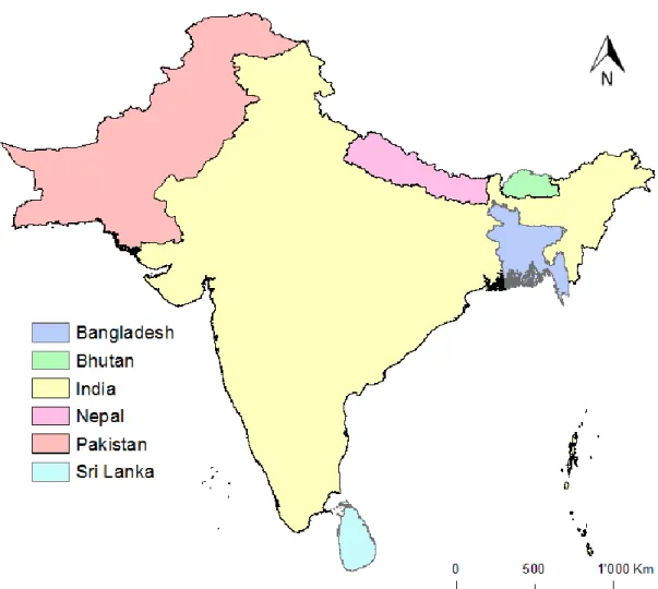
A

The study area is composed by the Indian peninsula and its surrounding countries, Pakistan, Nepal, Bhutan, Bangladesh and also Sri Lanka, comprising a total area of 4,564,713Km2, with an average population density of 364.76 people per Km2.

In general, temperatures tend to be higher and less variable when closer to the equator. The farther north from the equatorial line, the colder and uneven becomes the temperature along the year. The Himalayas act as a barrier to the frigid katabatic winds (cold wind that blows downhill across sloping ground (Allaby, 2007)) flowing down from Central Asia, keeping the most of the Indian subcontinent warmer than most locations at similar latitudes (Attri & Tyagi, 2010).

9

2.1.1 India

The Indian Territory is the largest (3,287,590 Km2), with a human population density of 384.3 people/Km2, and characterized by very different climate regions, ranging from a Mountain climate on the north-west of India (where temperatures range from 0ºC to 18ºC and climate may vary from nearly tropical in the foothills to tundra, above the snow line, depending on altitude) (Singh & Kumar, 1997) to Tropical wet (where the average temperature is higher than 18ºC during the colder, drier, months and can exceed 50ºC during the summer, with annual rainfall averaging from 750 to 2,000 mm) (Attri & Tyagi, 2010).

Winter time corresponds to January and February (and also December in the north-western part of India) and is characterized by clear skies and low humidity and temperatures. This is also the driest season of the year, with very few mm of rain, and mostly over the western Himalayas (Attri & Tyagi, 2010).

Summer season (or pre-monsoon quarter) extends from March to May, when temperatures increase all over the Indian Territory and. maximum temperatures rise sharply by the end of May/beginning of June, which results in harsh summers in the north and north-west regions. This season is also characterized by thunderstorms (Attri & Tyagi, 2010).

The Monsoon quarter, which is both the wettest and coldest time of the year, extends from June to September, accounting for about 75% of the annual rainfall (Attri & Tyagi, 2010). The monsoonal rainfall oscillates between active spells and breaks. Although it rains very little during the Breaks, these are associated with high humidity and temperatures (Attri & Tyagi, 2010).

Finally, the post-monsoon season (or North-East monsoon season), from October to December, is characterized by brighter weather in most of the country and daily temperatures start falling on all Indian Territory. Both pre and post-monsoon seasons account for about 11% of the annual rainfall (Attri & Tyagi, 2010).

2.1.2 Pakistan

Pakistan is the second largest country of the study area, with a total area of 880,940 Km2 and a human population density of 260.8 people/Km2.

The climate varies from tropical to temperate, with arid conditions dominating about half of its total area. There is a monsoon season with frequent flooding due to heavy rainfall (where about 75% of the annual rainfall is observed) and a dry season with significantly less rainfall or none at all. There are four distinct seasons: a cool, dry winter from December through March; a hot, dry spring from April through June; the summer rainy season (or monsoon season) from July through September, and the post monsoon period of October and November (Hussain & Lee, 2009).

2.1.3 Bangladesh

Although its area is about a sixth of Pakistan’s (143,998 Km2

), Bangladesh has almost as much inhabitants as that country, conferring it a very high average population density of 1,033.5 people/Km2.

Four distinct seasons can be recognized in Bangladesh: the dry winter season from December to February, where air temperature does not fall under 0 ºC, a pre monsoon hot summer season from March to May, a rainy monsoon season from June to September where 75% of annual rain falls, and a post-monsoon autumn season which lasts from October to November (Shahid, 2010).

2.1.4 Nepal

The dramatic differences in elevation found in Nepal result in a variety of biomes, from tropical savannas along the Indian border, to rock and ice at the highest elevations.(Lillesø, Shrestha, Dhakal, Nayaju, & Shrestha, 2005) Himalayan subtropical pine forests occur between 1,000 and 2,000 metres and temperate broadleaf forests from 1,500 to 3,000 metres. From 3,000 to 4,000 are the Himalayan subalpine conifer forests, and above 5,500 metres are the Himalayan alpine shrub and meadows (Bisht, 2008; Lillesø et al., 2005).

11 Its four seasons are divided as winter (December to February), pre-monsoon (March to May), monsoon (June to September), and post-monsoon (October and November) (Shrestha, Wake, Mayewski, & Dibb, 1999).

2.1.5 Bhutan

It’s the smallest country of the study area (38,394 Km2

), and also the one with the lower population density, with an average density of 19.3 people per Km2. Because Bhutan is very similar to Nepal in terms of geography and orography, their climate is also very similar (Davis & Li, 2013).

2.1.6 Sri Lanka

Sri Lanka is an Island located near the south-east coast of India. It has a total are of 65,610 Km2 and an average population density of 322 people per Km2. Although rainfall in Sri Lanka occurs throughout the year, it is under the influence of the Asian Monsoon system. For that reason, it has a heavier rain season from October to December; subsidiary rains from April to June and receives modest rainfall in the remaining drier months (Zubair, Siriwardhana, Chandimala, & Yahiya, 2007).

2.2 C

R

S

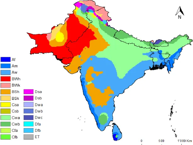
A

The first, and still the most widely-used, objective climate classification was developed by Köppen (1936), and was based on the concept that native vegetation is the best expression of climate. The strength of Köppen’s climate classification is that it considers different latitudinal zones (based on extreme temperatures) and seasonality in both temperature and precipitation (de Castro, Gallardo, Jylha, & Tuomenvirta, 2007; Peel, Finlayson, & McMahon, 2007). Figure 2 illustrates the Köppen climate classification for the study area.

Figure 2 - Climate regions (according to Köppen classification) present in the study area, taken from http://www.hydrol-earth-syst-sci.net/11/1633/2007/hess-11-1633-2007.html

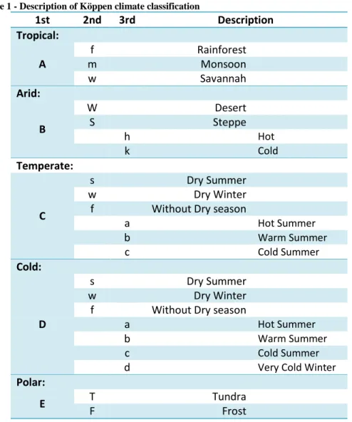
Table 1 presents a brief description of the classifications used by the Köppen climate scheme. There are a total of 30 different climate types divided into 5 major groups: tropical (A), arid (B), temperate (C), cold (D) and polar (E) (Peel et al., 2007).

Our study area is characterized by arid climates in the north-west, namely hot desert (BWh) and hot steppes (BSh). These can be described as having very low mean annual precipitation, too low to sustain vegetation (BWh) or just enough for short and scrubby vegetation (BSh). At the top north of the study area, a cold arid area (BWk) can be identified, where precipitation is still very low, but there is at least one month when the average temperatures fall below 0ºC.

13

Table 1 - Description of Köppen climate classification

1st 2nd 3rd Description Tropical: A f Rainforest m Monsoon w Savannah Arid: B W Desert S Steppe h Hot k Cold Temperate: C s Dry Summer w Dry Winter

f Without Dry season

a Hot Summer b Warm Summer c Cold Summer Cold: D s Dry Summer w Dry Winter

f Without Dry season

a Hot Summer

b Warm Summer

c Cold Summer

d Very Cold Winter

Polar:

E T Tundra

F Frost

India central and southern territory is characterized by a Tropical savannah (Aw) climate, with exception of the semi-arid climate area in the centre of this tropical region. This tropical climate area also extends into Bangladesh and continues to the Indian Territory in the upper east-coast of the study area and in the south-east coast to Sri Lanka. Tropical savannah climates have monthly mean temperatures above 18 ºC all year and typically a pronounced dry season, where less than 60mm of rain occur (McKnight & Hess, 2000).

Along the West Indian coast and immediately over the tropical savannah climate in the north-east limits of the study area, the climate is characterized by tropical monsoon (Am). Like tropical savannah, tropical monsoon climates have monthly mean temperatures above 18 °C during all year and feature wet and dry seasons. However, tropical monsoon

climate tends to see less variance in temperatures during the year than a tropical savannah climates do. This climate has a driest month which nearly always occurs at (or soon after) the winter solstice (McKnight & Hess, 2000).

In the south-west limit of Sri Lanka an area of tropical rainforest (Af) can clearly be observed. Tropical rainforests are a type of tropical climate in which there is no dry season and all months have an average precipitation value of at least 60mm. Tropical rainforests also have no summer or winter; are typically hot and wet throughout the year and rainfall is both heavy and frequent (McKnight & Hess, 2000).

In the north and central areas of India, continuing to the north limits of the study area, climate is characterized by a temperate “dry winter, hot summer” (Cwa) climate type, i.e. a humid subtropical climate, that transforms to a subtropical highland (temperate “dry winter, warm summer” – Cwb) climate along the study area’s north limit. This climate type can also be found in the south of the Indian peninsula. Humid subtropical climate is characterised by very hot (usually humid) summers that tend to be long (with high temperatures often exceeding 40 °C) and mild to cool winters that are dry and relatively short.

Finally, a small hot-summer Mediterranean climate (temperate “dry and hot

summer” – Csa) can be observed in the west limit of Pakistan, in yellow. Regions with this form of Mediterranean climate experience average monthly temperatures over 22.0 °C during its warmest month and an average between 18 and 0 °C in the coldest month. Hot, sometimes very hot and dry summers that can closely resemble summers seen in arid or semi-arid climates, and mild, wet winters are expected. High temperatures during summer are generally not as high as in arid or semiarid climates due to the presence of a large body of water.

3.1 S

M

M

Taking into consideration the aims of the project, the use of statistical models to predict the occurrence of the selected rodents (Ecological Niche Models, or ENMs) is a crucial approach. Having in mind that the amount of available data is small and most is restricted to presence-only occurrences, with no absence data recorded, an adequate SDM to use are Maximum entropy models (commonly known as Maxent models) (S. J. Phillips, Anderson, & Schapire, 2006). The Maxent models allow us to predict species occurrence probability using only its presence data through the use of environmental and/or spatial site characteristics, therefore maximizing the utility of the available resources (Elith, Phillips, Hastie, & Dudík, 2011; S. J. Phillips et al., 2006). Maxent models have also proven to work relatively well with small and clustered sample sizes, such as the ones used in this thesis (Kramer-Schadt et al., 2013; Kumar & Stohlgren, 2009; S. J. Phillips et al., 2006).

3.2 S

S

,

D

C

P

We first reviewed literature on small felids’ trophic ecology in South and Southeast Asia and collected data regarding rodents’ species preyed by wildcats. However, identification of prey at the species level is scarce and/or geographically limited. Therefore, we decided to cluster the data using genus as the lowest taxonomic category considered.

We searched online databases (e.g. Web of Knowledge) and reviewed available publications (e.g. ISI papers, books, project reports) that might have reported rodent’s presence data within Indian subcontinent. All records prior to 1970 were discarded in an attempt to decrease the mismatch between the presence records and the environmental data used (e.g. climate, land cover, human density), mostly from the late 90s. Due to the extensive size of the study area (4,444,046 Km2) and the imprecision of the rodent’s locations, a resolution of 5 arc-minutes was used for every non-vector variable (i.e. each pixel represented an area of approximately 10Km2).

Because there is no indication of rodent species preferred by small cats, we clustered the data into different body-weight classes that are likely to represent different

17 data. We organized the data in two groups: Weight Classes (“Small”, “Medium” and “Large”); and “Rodents’ Total” (all presence data).

3.2.1 Presence data

Data were collected for the genus Apodemus, Bandicota, Cannomys, Golunda, Leopoldamy, Mus, Nesokia, Niviventer, Rattus, and Tatera, according to the species referenced in the literature as wildcat prey (to see all used species check the ANNEXES section). The presence-only data were gathered from: the online database GBIF (“Occurrence Download - GBIF”); a broad rodent census taken for all South-Asian territory (Molur et al., 2005) and a non-systematic survey of rodents implemented by Krishnapriya Tamma (unpublished results). After merging all three sources of presence data, duplicated occurrences (by species in the 10Km2 grid cells) were removed, as well as those with erroneous or inaccurate geo-referenced locations. The global occurrences data set was reorganized and sub-divided into two subsets of data, representing the distinct types of analytical strategies: 1) Weight Classes where all data was divided into three different classes according to the species’ weight; and 2) all presence data together in a single “Rodents’ Total” group. Within each of these subsets, duplicates were also removed to allow an evaluation the occurrences sample size to be tested. The construction of models for each genus was not attempted due to extremely low sample sizes for some genus.

3.2.1.1 Weight Classes

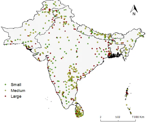
This data subset consists of the division of all presence data into three classes according to the species’ weight: small, medium or large. This division was made as suggested by the field specialists consulted, given into account that wildcats are opportunistic predators, and will most likely hunt the larger, easier to spot, preys other than smaller and more elusive ones (André Pinto da Silva, 2011; Nowell & Jackson, 1996; Rajaratnam, Sunquist, Rajaratnam, & Ambu, 2007b; Sakaguchi & Ono, 1994). The three weight classes range were based on a histogram of all used species’ weights (M Pacifici et al., 2013; Michela Pacifici et al., 2013), through which is possible to distinguish three separate classes: less than 70g (small) and more than 70g and less than 150g (medium). All species with more than 150g were considered large (Table 2 and Figure 3).

Table 2 - Weight classes range, showing weight intervals for each class.

Class Weight interval

Small ≤ 70g

Medium ]70g, 150g] Large > 150g

Figure 3 - Frequency of species per 5g class of body weight. The first red circle denotes the “Small” group; second circle denotes “Medium” and the remaining 5g classes make the “Large” group.

We identified a total of 47 different species preyed by wildcats, of which 22 species were classified in the “small” class (n = 314), 15 species in “medium” (n = 242) and 10 species in “large” (n = 247), all distributed throughout the study area (Figure 4).

0 1 2 3 4 5 6 5 _{25 45 65 85} 105 125 145 165 185 205 225 245 265 285 305 325 345 365 385 405 425 445 465 485 505 525 545 565 585 N u m b er o f speci es Weight (g)

19

3.2.1.2 Rodents’ Total

This group consists of all occurrence data available joined together, treated as a single group. There are a total of 580 occurrences, after duplicates removal. All presence data (by weight classes and grouped as rodents) were processed with the software Microsoft Office Excel, with the exception of the deletion of all erroneously geo-referenced occurrences (all occurrences which coordinates were outside the study area maps). This operation was accomplished using a binary mask to cut the occurrences (vectorial) layer to the size of the study area in software ArcGIS 10.2.2.

3.2.2 Independent variables

The independent data used to test the considered hypothesis in (i.e. Land cover, anthropogenic, altitude and climate variables) were collected, in a raster format, from various online data-bases:

Land cover data were collected from Global Land Cover 2000 (with an original

resolution of 1Km by the equatorial line) (“Global Land Cover 2000”), population density data were taken from the NASA SEDAC project (Socioeconomic Data and Applications Center) (with an original resolution of 2.5’) (“Downloads » Population Density Grid, v3: Gridded Population of the World (GPW), v3 | SEDAC”) and bioclimatic variables (temperature and precipitation), as well as altitude, were collected from WorldClim (with an original resolution of 5’) (“Bioclim | WorldClim - Global Climate Data”). Countries’

administrative boundaries, in vector format, were collected from DIVA-GIS database

3.2.2.1 Land Cover

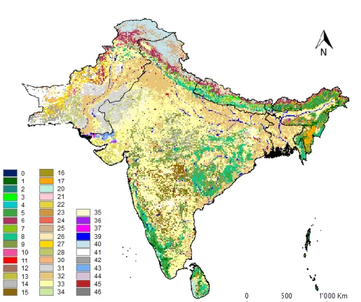
Land cover data consisted of a categorical (discrete) single raster layer composed by 46 land cover classifications, plus a classification for land with no cover data (Table 3; Figure 5).

Table 3- Categorical classes of the raster and its respective land cover description

0 Sea 16 Shrubs 32 Intensive Agriculture

1 Tropical Evergreen 17 Abandoned Jhum 33 Irrigated Agriculture 2 Subtropical Evergreen 18 Sparse woods 34 Slope Agriculture 3 Temperate Broadleaved 19 Bush 35 Rainfed Agriculture 4 Tropical Montane 20 Coastal vegetation 36 Current Jhum 5 Tropical Semievergreen 21 Savannah 37 Swamp 6 Temperate Conifer 22 Plain Grasslands 38 Coral reef 7 Subtropical Conifer 23 Slope Grasslands 39 Water Bodies 8 Trop. Moist Deciduous 24 Desert Grasslands 40 Snow

9 Trop. Dry Deciduous 25 Alpine Meadow 41 Barren 10 Junipers 26 Alpine Grasslands 42 Bare Rock 11 Mangroves 27 Sparse vegetation (cold) 43 Salt Pans 12 Degraded Forest 28 Sparse vegetation (hot) 44 Mud Flats

13 Dry Woodland 29 Gobi 45 Settlements

14 Scrub (Northern) 30 Desert (cold) 46 No Data 15 Scrub (Southern) 31 Desert (hot)

21

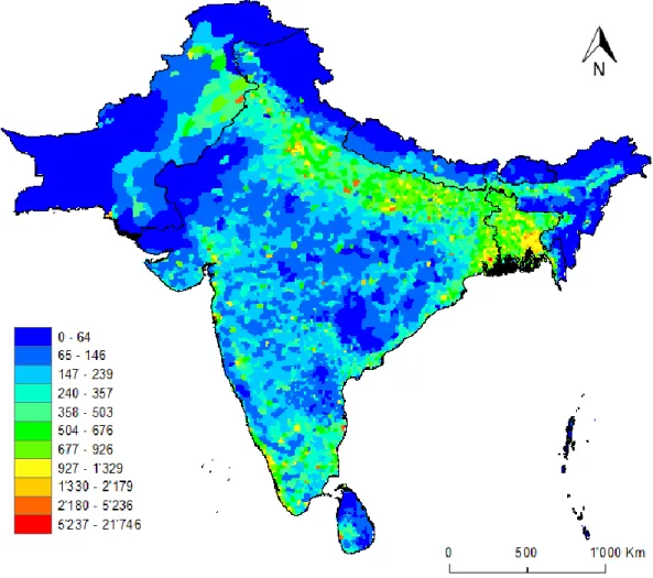
3.2.2.2 Population Density

Human population density is a continuous raster variable where values range from 0.09 to 21,746 persons per Km2 (Figure 6).

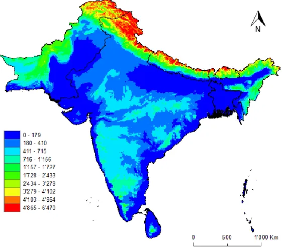
3.2.2.1 Altitude

It’s a continuous raster where values range from 0 to 6’500 meters above the sea level (Figure 7).

Figure 7 - Altitude variation (in meters) of the study area, where blue is 0m above the sea level and red is more than 4,865m above sea level.

23

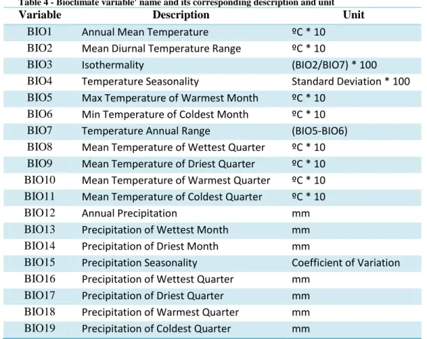
3.2.2.2 Bioclimate

Bioclimate variables correspond to a group of 19 temperature and precipitation related variables, (Table 4). Precipitation variables are presented in mm of rain and temperature is shown in ºC multiplied by 10 (e.g. a value of 231 represents 23.1ºC) (“Data format | WorldClim - Global Climate Data”).

Table 4 - Bioclimate variable' name and its corresponding description and unit

Variable Description Unit

BIO1 Annual Mean Temperature ºC * 10 BIO2 Mean Diurnal Temperature Range ºC * 10

BIO3 Isothermality (BIO2/BIO7) * 100

BIO4 Temperature Seasonality Standard Deviation * 100 BIO5 Max Temperature of Warmest Month ºC * 10

BIO6 Min Temperature of Coldest Month ºC * 10 BIO7 Temperature Annual Range (BIO5-BIO6) BIO8 Mean Temperature of Wettest Quarter ºC * 10 BIO9 Mean Temperature of Driest Quarter ºC * 10 BIO10 Mean Temperature of Warmest Quarter ºC * 10 BIO11 Mean Temperature of Coldest Quarter ºC * 10

BIO12 Annual Precipitation mm

BIO13 Precipitation of Wettest Month mm BIO14 Precipitation of Driest Month mm

BIO15 Precipitation Seasonality Coefficient of Variation BIO16 Precipitation of Wettest Quarter mm

BIO17 Precipitation of Driest Quarter mm BIO18 Precipitation of Warmest Quarter mm BIO19 Precipitation of Coldest Quarter mm

These variables were primarily tested for multicolinearity with the use of the tool “Band Collection” of ArcMap and its results were then analysed using Excel. All variables with a correlation value of more than 0.70 (Hosmer & Lemeshow, 2000) were carefully chosen or removed according to its relative importance to the present study (“Desktop Help 10.0 - How Band Collection Statistics works”). This resulted in two distinct sets of bioclimate variables (Table 5), focused mostly on monthly variables (Set1) and on quarterly and yearly variables (Set2). Bioclimate set 1 is expected to have the most valuable information regarding the rodent’s needs (S. Phillips, 2005), as it includes mainly monthly variables. However, literature revealed that broader variables, such as the annual and

quarterly variables from set 2, produce a better transferable model, allowing better predictions when the same model is used with future climate data or in new geographical areas (S. Phillips, 2005), which is crucial to understand potential responses to future climatic modifications.

Table 5 - Each bioclimate variables’ set, where Set 1 focuses mostly on monthly variables and Set 2 focuses on quarterly and yearly variables

Bioclimate Set 1 Bioclimate Set 2

BIO2 Mean Diurnal Temperature Range BIO4 Temperature Seasonality

BIO5 Max Temperature of Warmest Month BIO8 Mean Temperature of Wettest Quarter

BIO6 Min Temperature of Coldest Month BIO9 Mean Temperature of Driest Quarter

BIO13 Precipitation of Wettest Month BIO15 Precipitation Seasonality

BIO14 Precipitation of Driest Month BIO16 Precipitation of Wettest Quarter BIO18 Precipitation of Warmest Quarter BIO17 Precipitation of Driest Quarter BIO19 Precipitation of Coldest Quarter BIO18 Precipitation of Warmest Quarter

--- BIO19 Precipitation of Coldest Quarter

For the above mentioned reasons, and even though tests were run for both sets (with similar final results), only set 2 tests will be presented in the next chapters.

3.2.3 Independent variables set

Due to the differences in all independent variables resolution and the statistical analytic assumption that all data should have the same resolution, all variables were converted to the same 5 arc-minutes (or 5’) resolution, corresponding approximately to 10Km2, using a bioclimate raster as basis (all other rasters where converted to that bioclimate raster’s resolution). Following the resolution conversion, all raster variables were cut to fit the study area through the use of a binary mask. The binary mask was constructed in two phases: a “pre-mask” was created through the connection of each country’s administrative boundaries (“Download data by country | DIVA-GIS”). Following the “pre-mask” construction, one raster layer (already in 5’) was cut by this “pre-mask”, setting all values outside the study area to 0 and maintaining all original raster values within the study area. This cut raster was then divided by itself in order to obtain the binary mask (where all pixels inside the study area have the value 1 and all other have the value 0) to be used in the cutting of all other raster layers. This ensures that all layers will have the

25 exact same total number of pixels, a mandatory condition for the statistical software to run an analysis.

After all raster layers were cut to the same exact size, they were converted to ASCII format and saved as inputs to the Maxent software, together with the presence data’ csv file. All operations were made using the software ArcMap, from ArcGIS 10.2.2 (“ArcGIS for Desktop”).

3.3 S

A

3.3.1 Maxent input

The final data used as input for the Maxent software (“Maxent software and datasets”) were the independent variables described above (landcover, population density and altitude), together with bioclimate set 2 (a total of 11 independent variables) and each presence data file (“Small”, “Medium”, “Large” and “Rodents’ Total”), totalling 4 distinct analysis.

Maxent software allows the user to configure a large array of parameters in order to make the final model most suitable for the work in question. The importance and functioning of those parameters can be found in “A Brief Maxent Tutorial” (S. Phillips, 2005). After several test runs to better understand how each parameter influenced the generated models, the parameters modified from Maxent’s default Settings (Table 6) were the following:

Table 6 - Maxent parameters that were modified to fit this study aims

Maxent parameter Value

Random seed True

Random test percentage 30% Regularization multiplier 2

Replicates 50

Replicated run type “Subsample” Maximum iterations 5000

With “Random seed” set to True, Maxent will generate a new set of random test points for each replicate. If it was set to False, the same random test points would be used for every run. “Random test percentage” denotes how much (random) presence data will be used for model testing, percentage wise. “Regularization multiplier” will influence how closely fitted the output distribution is. A smaller value will result in an over-fitting to the training data, so the model won’t generalize well to independent test data (S. Phillips, 2005). The option “Create response curves” was also selected as it allows for an evaluation of each variable influence on the generated model.

3.3.2 Maxent Output

Given all the selected settings, Maxent software will then run as many model replicates as specified (50 in this case) using sets of randomly selected points from the inputted presence data together with a random points selection (30% of the presence data) used as training data. After all the replicates are complete, Maxent will then average all its results into a single model result output.

Maxent’s output consists in a visual representation of its final model (“Pictures of the model”), plus a set of other data explaining it in detail, all compiled into a single summary html page. The next topics will consist in a brief explanation of all Maxent output data used to achieve this works’ study aims.

27

3.3.2.1 ROC curve and AUC value

The first information given by Maxent is the receiver operating characteristic (ROC) curve (averaged over the replicate runs) which illustrates the model’s predictive power by comparing its sensitivity (ratio of how many times the test points were correctly chosen as a “presence” over all points chosen as presences) to its specificity (ratio of how many times test points were chosen as a “probable absence” over all points chosen as absences) (Pearce & Ferrier, 2000). The AUC (area under ROC curve) value is a single value consisting of the integral of the ROC curve. This ensures a single value for a better evaluation of the model’s predictive power. According to Manel et al (2001), generated Maxent models with AUC values of 0.5–0.7 are taken to indicate low accuracy, values of 0.7–0.9 indicate useful applications and values of > 0.9 indicate high accuracy (Manel, Williams, & Ormerod, 2001).

3.3.2.2 Variable contributions and Response curves

Maxent presents, among others, a table with each variable relative contribution to the final model. These are the average values over the total replicate runs. The response curves show how each variable affects the Maxent prediction by varying its value while keeping all other variables at their average value. When running multiple replicates, the final model’s response curves show the average value of all replicates in red and the standard deviation in blue.

The results for each analysis (i.e. per weight class and all rodents) and the variables with the highest percent contribution will be presented in the following sections. All the best models produced for each category of data can be considered to have useful applications and medium accuracy, since all AUC values were > 0.7 (Table 7) (Manel et al., 2001).

Table 7 - AUC values for each run analysis

Tested data AUC (average value of the 50 runs) Standard deviation “Small” 0.753 0.031 “Medium” 0.752 0.019 “Large” 0.774 0.023 “Rodents’ Total” 0.741 0.015

The average AUC values for the different model categories are quite similar, with low standard deviations, indicating that the AUC values didn’t vary much over the replicate runs of the models. The “Large” category data models had the highest AUC value, whereas the lowest value corresponds to the “Rodent’s total” analysis.

4.1 C

“S

”

Figure 8 illustrates the final Maxent model for the small-size rodents’ data (less than 70g). There are a few areas with a high probability of occurrence (where values are higher than 0.77), mainly along the northern part of Pakistan, India and Nepal, centre of Bangladesh and the southwest of Sri Lanka. Most red “dots” across all study area, representing high probability of small mammals’ presence, correspond to major cities, such as Islamabad in northern Pakistan, Kathmandu in Nepal or Mumbai in India.

31

Figure 8 - Model representation showing the probability of occurrence of small-size rodents over all the study area.

Southwest Pakistan and the upper north corner of India denote a very low probability of occurrence, below 0.15. It is clear that central India also shows a somewhat low probability of occurrence, even though it didn’t reach the low values previously mentioned (below 0.35). India’s west coast shows the same low occurrence probability observable in central India; the exception is Mumbai city appearing in yellow and bright red (above 0.77).

The independent variables that have a higher contribution to the small rodents’ Maxent model (i.e. higher influence in species’ presence) are land-cover classes, and four bioclimate variables: Bio 17 (precipitation of the driest quarter) seems to have a higher influence, but Bio 4 (temperature seasonality), Bio 15 (precipitation seasonality) and Bio 19 (mean temperature of the driest quarter) also have high contribution values (Table 8).

Table 8 - Percentage of relative importance of each independent variable to the final Maxent model

Variable Percent contribution (%)

land_cover 25.2 bio17 22.1 bio4 14.1 bio15 12.4 bio19 11.2 Altitude 6.5 Pop_dens 2.7 bio18 2.6 bio16 1.9 bio9 0.7 bio8 0.6

The highest contributing variables show distinct influence patterns, i.e. different response curve shapes (Figure 9 and Figure 10). Since land cover is a categorical variable, its response curve is actually a bar graph showing the probability of presence (of small rodents) for each class. “Settlements” areas (class 45) present a probability of occurrence higher than 0.9 (Figure 9). Moreover, although “dry woodland” categories (class 13) have a high standard deviation value, it is still regarded as important, with a high (average) probability of occurrence, i.e. higher than 0.8.

Figure 9 - Probability of presence according to the Maxent model for each land-cover class. Red bars denote the average value over all 50 replicates and blue bars represent the standard deviation.

33 The response curves of the most influential bioclimate variables show that when the precipitation of the driest quarter increases (Bio 17), so does the probability of presence of small rodents (Figure 10). In turn, when the temperature seasonality value (Bio 4) is increased, the probability of presence of small rodents decreases. Rodent occurrence seems also to decrease faintly when precipitation seasonality (Bio 15) rises, until 150mm of rain, and rise slightly from this point forward. Moreover, rodent occurrence rises along with the precipitation of the coldest quarter (Bio 19), although never reaching a 0.9 probability of occurrence and with great standard deviation values.

Figure 10 - Response curves for variables Bio 17, Bio 4, Bio 15 and Bio 19 for small rodents’ model (in red; Blue shaded areas represent the standard deviation). Ordinate axis corresponds to probability of occurrence. Abscissa axis values are presented in the corresponding variable units (see Table 4)

4.2 C

“M

”

The visual representation of the model for medium size rodents (between 70g and 150g) is somewhat similar to the small rodents’ model (Figure 8 and Figure 11), the main difference being a higher probability of occurrence in Sri Lanka. It also shows a slightly lower probability of occurrence in the north-western part of the study area and slightly higher in Nepal. A higher occurrence probability in major cities remains alike, i.e. values reaching 1. The areas with a low probability of occurrence remain the same as in the small rodents’ model.

Figure 11 - Model representation showing the probability of occurrence of medium-size rodents over all study area.

35

Table 9 – Percentage of relative importance of each independent variable to the final medium rodents’ Maxent model

Variable Percent contribution (%)

land_cover 30.6 bio4 22.1 bio19 16.7 bio15 8.3 altitude 5.4 bio17 5.2 bio18 4.8 Pop_dens 2.5 bio9 2 bio16 1.9 bio8 0.4

Moreover, the response curves of the most important variables for this model also show some differences (Figure 12 and Figure 13). Once again, the land cover classes that are linked to a higher probability of presence are “settlements” (Class 45) and “dry woodland” (Class 13), even though its rodents’ presence probability value is much lower than that estimated for “settlements” (class 45), 0.94 and 0.79 respectively.

Figure 12 - Probability of presence of medium-size rodents (according to its Maxent model) for each land-cover class. Red bars denote the average value over all 50 replicates and blue bars represent the standard deviation.

The bioclimate variables show more similar patterns with temperature seasonality values (Bio 4) being negatively related with the probability of presence for medium sized rodents decreases. As for the precipitation of the coldest quarter (Bio 19), presence probability rises until prox. 1500mm of rain, but decreases to 0.5 when precipitation values increase above that value.

4.3 C

“L

”

The model for large-size rodents (more than 150g) produced the most distinct distribution probability map of all generated weight models (Figure 14). This model presents more defined areas and contours, i.e. the spots marked as high probability presences (values close to 1) are well defined and with almost no yellow “circles” around them (lower probability). The same is true for areas with a lower probability of occurrence: the areas that appear blue (with values close to 0) are wider and easily identifiable.

Figure 13 - Response curves for variables Bio 4 and Bio 19 for the medium rodents’ model (in red; Blue shaded areas represent the standard deviation). Ordinate axis corresponds to probability of occurrence. Abscissa axis values are presented in the corresponding variable units (see Table 4)

37

Figure 14 - Model representation of the probability of occurrence for large-size rodents over all study area.

There is an increased probability of occurrence along the coast line, and a more defined smaller area of Sri Lanka with a high occurrence probability in comparison with the previously presented models. If we observe Sri Lanka more closely, it is easy to identify two main cities where the highest occurrence probability is shown (Colombo and Kandy), whereas in the previous models most of the island was classified as a high occurrence probability area, where no particular city was distinguishable. All the north line of the study area, corresponding to the Himalayas mountain range, is shown as bright blue, denoting zero probability of occurrence according to the Maxent model results.

The independent variables that contributed more to the Maxent model for large-size rodents are land-cover classes, population density and altitude (Table 10). The bioclimate variable Bio 4 (temperature seasonality) also appears to have a high contribution for the model. These results further shows that the model built for large-size rodents differs from the previous rodents’ models.

Table 10 – Percentage of relative importance of each independent variable to the final large rodents’ Maxent model

Variable Percent contribution (%)

land_cover 27.9 Pop_dens 19.2 Altitude 15.3 bio4 14.1 bio18 8.2 bio17 5 bio16 3.4 bio15 2.4 bio19 1.7 bio9 1.6 bio8 1.2

The individual analyses of the highest contributing variables show different influential patterns between them (Figure 15 and Figure 16). Although the components of this model differ from the previous ones, land cover is still the most influential variable. The most important class is, again, “settlements” (Class 45), with an associated probability of occurrence of 0.9. However, “dry woodland” category (Class 13) is no longer as important, and there are no other classes with high associated probabilities of occurrence (i.e. higher than 0.7) (Figure 15).

39

Figure 15 - Probability of presence of large rodents (according to its Maxent model) for each land-cover class. Red bars denote the average value over all 50 replicates and blue bars represent the standard deviation.

Figure 16 shows that large-size rodents’ probability of presence increases strongly when population density in increased from 0 to 5000 people per Km2, almost reaching the value of 1 above this value. Moreover, although it has almost no effect until the 2500m

Figure 16 - Response curves of the variables Population density, Altitude and Temperature Seasonality for the large rodents’ model (in red; Blue shaded areas represent the standard deviation). Ordinate axis corresponds to probability of occurrence. Abscissa axis values are presented in the corresponding variable units (see chapter 3.2.2)

above the sea level, the altitude response curve shows that, as altitude increases above that value, the probability of presence for large-size rodents decreases to almost 0. Temperature seasonality’s influence remains the same as for the previous models.

4.4

“R

’

T

”

The model produced by clustering all the data into a unique class (Rodents) is very similar to the “medium weight” model, the most significant differences being for the west India coast, which appears with an approximate value of 0.3 instead of almost 0. It is also evident that this model image is less defined than the others. For example, the lowest probability areas are not well defined.

41 A higher probability of occurrence in Sri Lanka is again visible, occupying a significant part of this island. North-western India and Nepal gained a greater importance, appearing with occurrence probabilities of 0.7 and higher. Again, Central and north-western regions show the lowest probability of rodents’ presence.

The independent variables that have a higher contribution to this Maxent model are land-cover classes and the bioclimate variables Bio 4 (temperature seasonality), Bio 19 (precipitation of the coldest quarter) and Bio 17 (precipitation of the driest quarter) (Table 11).

Table 11 – Percentage of relative importance of each independent variable to the final rodents’ total Maxent model

Variable Percent contribution (%)

land_cover 31.4 bio4 22.3 bio19 11.6 bio17 11.5 altitude 7.3 bio15 6.5 Pop_dens 4.2 bio18 3.4 bio16 1.1 bio9 0.6 bio8 0.3

The land cover class that is associated to a higher probability of rodents’ presence is again “settlements” (Class 45), with a probability of 0.9. Moreover, the “dry woodland” (Class 13) seem also to be important, even though its presence probability value is lower - 0.7 (Figure 18).

Figure 18 - Probability of presence of rodents (according to its Maxent model) for each land-cover class. Red bars denote the average value over all 50 replicates and blue bars represent the standard deviation.

Regarding bioclimatic variables, as temperature seasonality values increase (Bio 4), the rodents’ probability of presence decreases (Figure 19). Regarding the precipitation of the coldest quarter (Bio 19), presence probability rises until c.a. 1500mm of rain, but decreases to 0.6 when precipitation values increase above the referred value. As the precipitation of the driest quarter increases (Bio 17), so does the probability of occurrence of rodents.