ESSAYS ON THE USE OF THE REAL OPTIONS APPROACH
IN CONSTRUCTION PROJECTS AND BUILD-OWN-TRANSFER PROJECTS
por
João Adelino Neves Pereira Ribeiro
TESE DE DOUTORAMENTO EM CIÊNCIAS EMPRESARIAIS
Orientada por:
Sr. Prof. Doutor Paulo Jorge Marques de Oliveira Ribeiro Pereira Sr. Professor Doutor Elísio Fernando Moreira Brandão
Deste modo ou daquele modo.
Conforme calha ou não calha.
Podendo às vezes dizer o que penso,
E outras vezes dizendo-o mal e com misturas,
Vou escrevendo os meus versos sem querer,
Como se escrever não fosse uma cousa feita de gestos,
Como se escrever fosse uma cousa que me acontecesse
Como dar-me o sol de fora.
Procuro dizer o que sinto
Sem pensar em que o sinto.
Procuro encostar as palavras à idéia
E não precisar dum corredor
Do pensamento para as palavras
Nem sempre consigo sentir o que sei que devo sentir.
O meu pensamento só muito devagar atravessa o rio a nado
Porque lhe pesa o fato que os homens o fizeram usar.
Procuro esquecer-me do modo de lembrar que me ensinaram,
E raspar a tinta com que me pintaram os sentidos,
Desencaixotar as minhas emoções verdadeiras,
Desembrulhar-me e ser eu, não Alberto Caeiro,
Mas um animal humano que a Natureza produziu.
E assim escrevo, querendo sentir a Natureza, nem sequer como um homem,
Mas como quem sente a Natureza, e mais nada.
E assim escrevo, ora bem ora mal,
Ora acertando com o que quero dizer ora errando,
Caindo aqui, levantando-me acolá,
Mas indo sempre no meu caminho como um cego teimoso.
Ainda assim, sou alguém.
Sou o Descobridor da Natureza.
Sou o Argonauta das sensações verdadeiras.
Trago ao Universo um novo Universo
Porque trago ao Universo ele-próprio.
Isto sinto e isto escrevo
Que são cinco horas do amanhecer
E que o sol, que ainda não mostrou a cabeça
Por cima do muro do horizonte.
Ainda assim já se lhe vêem as pontas dos dedos
Agarrando o cimo do muro
Do horizonte cheio de montes baixos.
À memória da minha mãe, Margarida.
Nota Biográfica
João Adelino Neves Pereira Ribeiro nasceu no dia 25 de Setembro de 1967, em Guimarães.
Em Outubro de 1990 completou a licenciatura em Gestão de Empresas, na Universidade Portucalense Infante D. Henrique, com média final de 15 valores. Em Janeiro de 1992 terminou o programa de mestrado “Master of Business of Admnistration” (M.B.A.) pela Universidade de Birmingham, Reino Unido, com a apresentação e aprovação da respectiva dissertação final, designada de “Capital Structure and Sources of Funds with Particular Reference to Portuguese Industrial Companies”. Em Novembro de 1996 obteve, por equivalência, o grau de mestre em Finanças pela Universidade Portucalense Infante D. Henrique.
Iniciou a sua actividade profissional no extinto Banco Português do Atlântico (Gabinete Central de Análise Económica e Financeira da Direcção Comercial Norte) em Outubro de 1992, tendo deixado de colaborar com esta instituição em Maio de 1993. No ano lectivo de 1992/93, iniciou a sua carreira académica, tendo assumido as funções de docente no Instituto Superior da Maia, onde leccionou, até 1994, as disciplinas de “Cálculo Financeiro” e de “Organização e Gestão de Empresas”. Na Universidade Portucalense Infante D. Henrique e respectivos Institutos Politécnicos, leccionou, desde o ano lectivo de 1993/94 até ao ano lectivo de 2004/05, as disciplinas de “Cálculo Financeiro”, “Contabilidade Geral”, “Análise Financeira”, “Auditoria Contabilística” e “Avaliação de Projectos de Investimento”, aos cursos de Contabilidade, Gestão de Empresas e de Administração Pública.
Exerceu funções de Direcção Financeira em duas empresas: “Galler Portuguesa - Fábrica de Malhas, Lda.”, subsidiária do grupo multinacional inglês “Courtaulds Textiles, PLC”, entre Outubro de 1994 e Abril de 1996 e, entre Junho de 1996 e Abril de 2005 em “Cari - SA”, empresa dedicada ao sector da construção civil e obras públicas. Foi também responsável, enquanto consultor, pela elaboração de diferentes estudos, com especial destaque para a execução de estudos de viabilidade económica e financeira no âmbito de candidaturas a difer-entes programas de incentivos ao investimento produtivo, actividade que desenvolveu entre os anos de 1992 e 1994 e, mais tarde, nos anos de 2008 e 2009.
Em Outubro de 2009 iniciou o programa de Doutoramento em Ciências Empresariais na Faculdade de Economia da Universidade do Porto. Completou, em Fevereiro de 2011, a componente escolar do programa com média final de 15 valores. Iniciou, então, os trabalhos conducentes à elaboração da presente tese de doutoramento. Em 2012, apresentou o primeiro dos artigos que integra esta dissertação em duas Conferências: na 7ª edição da “Portuguese Network Finance Conference”, realizada em Julho desse ano na Universidade de Aveiro e ainda na 6ª edição da “Portuguese Economic Journal Conference”, realizada no mesmo mês de Julho, na Faculdade de Economia da Universidade do Porto.
Acknowledgments
During this challenging - yet fascinating - period of my life, I was fortunate to have benefited from the friendship and support of several persons and institutions.
I address my first words to my supervisors, Professor Paulo Pereira and Professor Elísio Brandão.
My gratitude to Professor Paulo Pereira is endless. He has accompanied me since the first moment we talked, when I asked him to supervise my work. His positive response is the remote cause of the present dissertation. It was the combination of his passion for the field of real options with my prior professional knowledge about the construction industry and public contracting that has made this work possible. Without Professor Paulo Pereira outstanding commitment which went far beyond what I consider to be the standard supervisor requirements -this thesis would not have been written. I truly hope that our relationship as researchers will endure.
Professor Elísio Brandão has encouraged me so much, since the first time we talk about my possible decision of enrolling in this PhD program. From then onwards, Professor Elísio Brandão has always addressed me words of encouragement, and his example as an outstanding academic and researcher has been a source of inspiration until the present day. And I am sure that his example will keep inspiring me in the future.
I also wish to address words of deep gratitude to Professor José da Silva Costa, my first Lecturer of “Capital Budgeting and Investment Appraisal”, back in the years of 1989/90. Professor José da Silva Costa outstanding skills as a lecturer and the profound commitment to his students were the reasons why I felt a deep interest for this field of knowledge, more than 20 years ago.
Likewise, I owe words of profound gratitude to Professor Manuel Oliveira Marques for his continuous encour-agement and for always being available to help me in anyway I needed.
I also feel deeply in debt with Professor João Alves Ribeiro and Professor João Proença, former Directors of the PhD program. Both gave me useful advices before and during the taught part of the program. I am also thankful to Professor Carlos Cabral Cardoso for his availability and words of encouragement since he became the program Director.
I would like to gratefully thank all my colleagues with whom I have shared the same working space (the famous room 252) throughout a substantial part of the PhD program. I am especially grateful to Carlos Miguel Silva for his continuous support. His readiness to help me out when ever I needed is an irrefutable proof that companionship between PhD students is not a vain word. I am sure that we will stay friends forever.
I am also extremely grateful to Gonçalo Faria, Fabio Verona and David Nascimento for their continuous support and friendship. I extend my gratitude to Jurrien Bakker, Luis Silva, Rui Nascimento, José Pedro Fique, Fernando
Coelho and João Ricardo Costa Filho. All of them, in one way or another, made me a better researcher by sharing their knowledge with me. I also thank my friend Ricardo Lopes for the rich discussions about construction management and bidding competitions.
I am also in debt to Professor António Brandão, Professor João Correia-da-Silva, Professor Pedro Campos, Pro-fessor Jorge Farinha, ProPro-fessor Jorge Valente, ProPro-fessor Augusto Santos Silva and ProPro-fessor Paulo Vasconcelos for their valuable comments and useful suggestions in different moments of the research period.
To all my friends - inside and outside the Faculty premises - I am especially grateful for always being there for me, especially when times were difficult. I am particularly thankful to José Nobre, Andreia Santos Nobre, Luis Sampaio, Mónica Fernandes, Rui Maia, Paula Damião, Pedro Tenreiro, Nuno Mendes, Carla Coelho, Paulo Pimenta Machado, Filipe Macedo, Pedro Xavier, Marcos Tavares, Maria Tavares, Pedro Leal, Rui Leal, Adélia Pires, José Marques, Emídio Guerreiro, Joana Lopes, Joana Koehler, Carmo Afonso, Pedro Ricciardi, Rolando Sampaio, Vitor Ribeiro, António Teixeira, Carla Ramos, Vasco Leite, Renata Blanc, Ilda Castedo, Teresa Marinho Bianchi, Sandra Teixeira do Carmo, Ana Maria Medeiros, Liliana Ferreira, Cláudia Almeida Rodrigues, Álvaro Oliveira, Alexandre Coelho Lima, Fernando Cunha Guimarães Machado, Tânia Marques, Ana Carolina, Lau Alves, Pedro Cadima, Diana Monteiro, Álvaro Gonçalves, António Cordeiro, Ana Pacheco, Nuno Silva, Vicente Abreu, Carlos Moura, Pedro Pereira Neto, Ian Reynolds, Cazzie Antoinette, Tonya Meeks, Ghana Hilton, Ron Scott, Cecil Walters, Matt Velez, Jamal Kersey, Cliff Morehead, Jason Armitage, Blair Gilles, Rodney Williams and, surely, so many others. I hope they will excuse me for not being able to list their names.
I also thank the 7th Edition of the Portuguese Finance Network Conference and the participants for helpful comments. Especially, I am very grateful to Professor Dean Paxson for the insightful comments provided as Discussant of the paper presented in this Conference. Likewise, I thank the 6th Edition of the Portuguese Economic Journal Conference and the participants in the “Financial Economics” Panel for useful comments and suggestions.
I also acknowledge the financial support provided by FCT - Fundação para a Ciência e Tecnologia (Grant nº SFRH/BD/71447/2010) during a substantial part of the PhD program.
Last - but certainly not least - I am endlessly grateful to my father, António, my brother, Casimiro José, my nephew, Casimiro António and my cousin, Isabel, for their unconditional love and support. This work also belongs to them.
Resumo
Esta tese pretende ser uma contribuição para o corpo de investigação em torno da utiliza-ção da metodologia das opções reais a projectos de construutiliza-ção e a projectos de construutiliza-ção- construção-exploração. Pese embora estes projectos possuam uma natureza distinta da maioria dos restantes projectos de investimento, consideramos que comungam das características da irre-versibilidade, incerteza e flexibilidade.
Nos Capítulos II e III, propomos dois modelos teóricos de apoio à decisão que podem ser utilizados por gestores de empresas dedicadas à realização de projectos de construção ad-judicados através de um procedimento concursal competitivo. No Capítulo II, sugerimos um modelo que permite determinar o preço óptimo para a realização do projecto, baseado na avaliação de uma opção real por nós identificada e que apenas pode ser exercida pela empresa vencedora do concurso. No Capítulo III, estudamos os efeitos produzidos por um conceito específico de incerteza que rodeia os projectos de construção, e que designamos por “incerteza de volume”. Com base na solução numérica apresentada no Capítulo II, propomos um modelo que permite determinar o impacto esperado que este tipo de incerteza produz no preço óptimo, através da definição de uma variável estocástica designada por “valor adi-cional”, i.e., o lucro que poderá ser gerado considerando os efeitos da incerteza referida. O modelo determina uma regra de apoio à decisão da realização de investimento de carácter incremental em capital humano e tecnologia, o qual permite quantificar o impacto esperado que a incerteza de volume causará no valor do projecto.
No Capítulo IV, no âmbito de um projecto de construção-exploração, propomos um modelo teórico, baseado na existência de duas variáveis estocásticas, cuja finalidade consiste em determinar o valor óptimo para a penalidade legal a incluir pelo governo ou outras entidades públicas na minuta do respectivo contrato, no caso de a empresa concessionária não iniciar a execução do projecto imediatamente. O modelo contempla a existência de custos sociais e considera que a entidade privada é mais eficiente do que a entidade pública a construir a infraestrutura do projecto.
Abstract
The present thesis aims to contribute to the existent body of research dedicated to the use of the real options approach in construction projects and Build-Own-Transfer (BOT) projects. Even though these type of projects have a different nature than the majority of the other investment projects, we believe that they share the same characteristics of irreversibility, un-certainty and flexibility.
In Chapters II e III, we suggest two theoretical support decision models that may be applied by construction managers in the context of bidding competitions. In Chapter II, we pro-pose a model whose outcome is the optimal price for the execution of a construction project awarded through an appropriate bidding process. The model is based on the valuation of a specific real option, previously identified, and which can only be exercised by the selected bidder. In Chapter III, we study the effects of a particular type of uncertainty that surrounds construction projects, and which we designate as “volume uncertainty”. Applying the nu-merical solution presented in the previous Chapter, we suggest a model that addresses the expected impact of this type of uncertainty on the project value and on the optimal bid price, through the definition of a stochastic variable, designated as “additional value”, i.e., the profit that may be generated through the execution of additional work. The model’s outcome is the threshold value for the incremental investment in human capital and technology construction managers may undertake with the purpose of quantifying the expected impact that this type of uncertainty will produce on the project value.
In Chapter IV, we suggest a theoretical model to be applied by governments and other public entities, in the context of Build-Own-Transfer projects, based on a two-factor uncertainty approach in continuous-time, aiming to determine the optimal value for the legal penalty to be included in the contract form, in the case the selected bidder does not implement the project immediately. The model considers the existence of social costs and assumes that the private entity is more efficient than the public entity in executing the project facility.
Contents
1 Introduction 1
2 Reaching an Optimal Mark-Up Bid through the Valuation of the Option to Sign
the Contract by the Selected Bidder 8
2.1 Introduction . . . 8
2.2 The Model . . . 14
2.2.1 Introduction . . . 14
2.2.2 Assumptions . . . 14
2.2.3 Model Description . . . 15
2.2.3.1 The Value of the Option to Sign the Contract and Perform the Project . . . 15
2.2.3.2 The Probability of Winning the Bid . . . 17
2.2.3.3 The Optimal Price . . . 19
2.3 Numerical Example . . . 19
2.3.1 The Base Case . . . 19
2.3.2 Sensitivity Analysis . . . 22
2.3.2.1 Volatility . . . 23
2.3.2.2 ’Time to Expiration’ . . . 24
2.3.2.3 Construction Costs . . . 25
2.3.2.4 The Impact of Variations in Parameter ’b’ on the Option Value and on the Optimal Price . . . 26
2.3.2.5 The Impact of Variations in Parameter ’n’ on the Option
Value and on the Optimal Price . . . 26
2.4 Considering the Existence of Penalty Costs . . . 28
2.5 Conclusions and Remarks . . . 33
3 The Impact of Volume Uncertainty on the Project Value and on the Optimal Bid Price 35 3.1 Introduction . . . 35
3.2 Recognizing and Quantifying Hidden-Value: The Concept of Additional Value 39 3.2.1 Sources of Additional Value . . . 40
3.2.1.1 Extra Quantities . . . 40
3.2.1.2 Additional Orders . . . 41
3.2.2 Types of Contract . . . 42
3.3 How the Detection of Hidden-Value May Lead to Additional Value: Contrac-tor’s Opportunistic Bidding Behavior . . . 44
3.4 The Model . . . 46
3.4.1 Introduction . . . 46
3.4.1.1 The Value of Option to Sign the Contract and Invest in Performing the Project in the Presence of Penalty Costs . . 47
3.4.1.2 The Probability of Winning the Bid . . . 48
3.4.1.3 The Base Price . . . 49
3.5 Assumptions . . . 49
3.6 Model Description . . . 50
3.6.1 Introduction . . . 50
3.6.2 The Impact of the Non-Incremental Investment . . . 51
3.6.2.1 The Value of the Option to Sign the Contract and Perform the Project . . . 53
3.6.3 The Impact of the Incremental Investment in Human Capital and Technology . . . 54
3.6.3.1 The Optimal Price and the Value of the Option to Invest
Considering the High-Value Estimate . . . 55
3.6.3.2 The Optimal Price and the Value of the Option to Invest Considering the Low-Value Estimate . . . 55
3.6.4 The Threshold Value for the Incremental Investment . . . 56
3.7 Numerical Example . . . 57
3.7.1 The Base Case . . . 57
3.7.2 Sensitivity Analysis . . . 59
3.7.2.1 Is There a Scale-Effect? . . . 59
3.7.2.2 The Impact of Variations in the Probabilities Associated with the High/Low Value Estimates . . . 60
3.7.2.3 The Impact of Variations in the Difference Between the Two Estimates . . . 61
3.8 Conclusions and Remarks . . . 63
4 A Two-Factor Uncertainty Model to Determine the Optimal Contractual Penalty for a Build-Own-Transfer Project 65 4.1 Introduction . . . 65
4.1.1 Build-Operate-Transfer (BOT) Projects in the Context of Bidding Competitions . . . 65
4.1.2 The Real Options Approach in the BOT Projects Literature . . . 67
4.1.3 Two-Factor Uncertainty Models in the Real Options Literature . . . . 68
4.2 Proposed Framework . . . 70
4.2.1 Flexibility May Imply a Cost. The Contractual Penalty . . . 70
4.2.2 The Comparative Efficiency Factor . . . 71
4.2.3 Social Costs . . . 72
4.2.4 The Optimal Value for the Contractual Penalty . . . 73
4.3 The Model . . . 75
4.3.2 Model Description . . . 75 4.3.2.1 Introduction . . . 75 4.3.2.2 The Government Decision to Invest . . . 78 4.3.2.3 The Government Expectation about the Private Firm
In-vestment Decision . . . 81 4.3.2.4 Determining the Optimal Value for the Contractual Penalty 83 4.3.3 Sensitivity Analysis . . . 87 4.3.3.1 The Impact of Variations in the Level of Social Costs . . . 87 4.3.3.2 The Impact of Variations in the Level of the Efficiency Factor 88 4.3.3.3 The Combined Impact of Variations in the Level of Social
Costs and in the Level of the Efficiency Factor . . . 90 4.3.3.4 The Impact of Variations in the Correlation Coefficients . . 91 4.3.3.5 The Impact of Variations in the Standard Deviations . . . . 92 4.4 The Effects, to the Government, of a Including a Non-Optimal Value for the
Legal Penalty in the Contract . . . 93 4.4.1 The Effects of Including a Below-Optimal Penalty Value in the Contract 95 4.4.2 The Effects of Including an Above-Optimal Penalty Value in the
Con-tract . . . 98 4.5 Concluding Remarks . . . 101
5 Conclusion 104
A The Selected Bidder Decision to Invest 109
List of Figures
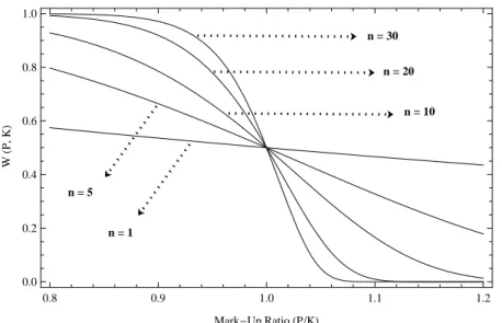
2.1 representation of the equation linking the mark-up ratio with the probability
of winning the bid, considering five different values for parameter ’n’ . . . . 17
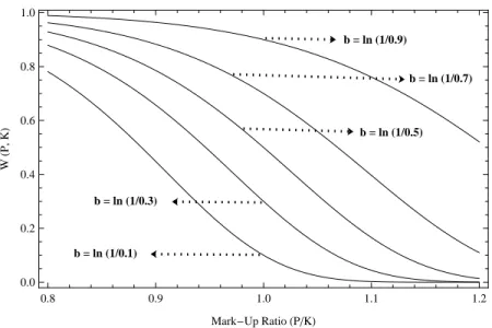
2.2 representation of the equation linking the mark-up ratio with the probability of winning the bid, considering five different values for parameter ’b’ . . . . 18
2.3 graphical representation of the equation linking the mark-up ratio with the probability of winning the bid, considering that parameter ’b’ equals ln(1/0.5) and parameter ’n’ equals 10 . . . 20
2.4 relationship between the price and the option value . . . 22
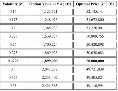
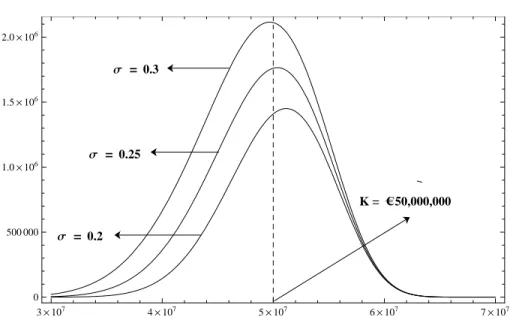
2.5 sensitivity analysis: volatility parameter . . . 24
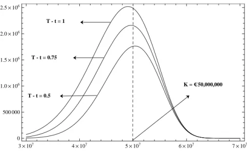
2.6 sensitivity analysis: ’time to expiration’ parameter . . . 25
2.7 relationship between the price and the option value, considering the existence of penalty costs . . . 31
2.8 relationship between the price and the option value, with and without the existence of penalty costs . . . 32
4.1 the government discriminatory boundary . . . 80
4.2 the impact of the optimal contractual penalty on the private firm discrimina-tory boundary . . . 85
4.3 the impact of overestimating the comparative efficiency on the optimal con-tractual penalty . . . 96
4.4 the impact of underestimating the comparative efficiency on the optimal con-tractual penalty . . . 99
List of Tables
2.1 inputs: description and values . . . 20
2.2 representative values for the mark-up ratio and the probability of winning the bid . . . 21
2.3 different results for the option value, considering different price levels . . . . 21
2.4 sensitivity analysis: volatility parameter . . . 23
2.5 sensitivity analysis: ’time to expiration’ parameter . . . 24
2.6 sensitivity analysis: construction costs . . . 25
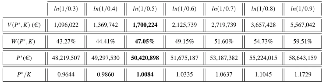
2.7 the impact of variations in parameter ’b’ on the option value and on the opti-mal price . . . 26
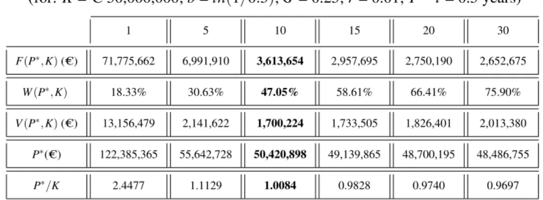
2.8 the impact of variations in parameter ’n’ on the option value and on the opti-mal price . . . 27
2.9 the impact of different prices on the option value and on the probability of winning the bid, in the presence of penalty costs . . . 31
2.10 the impact of different levels of penalty costs on the option value and on the optimal price . . . 32
3.1 inputs: description and values . . . 58
3.2 outputs: description, values and corresponding equations . . . 59
3.3 sensitivity analysis: scale-effect . . . 60
3.4 sensitivity analysis: probabilities associated with high/low value estimates . . 61
3.5 sensitivity analysis: difference between the high and the low value estimates . 62 4.1 the base case parameter values . . . 77
4.2 representative values for the government triggers, the private firm triggers and the optimal contractual penalty, for three project dimensions . . . 84 4.3 sensitivity analysis: the impact of variations in the level of social costs . . . . 87 4.4 sensitivity analysis: the impact of variations in the level of the efficiency factor 89 4.5 sensitivity analysis: the combined impact of variations in the level of social
costs and in the level of the efficiency factor . . . 90 4.6 the impact of variations in the correlation coefficients . . . 92 4.7 the impact of variations in the standard deviations . . . 93 4.8 the effects, to the government, of overestimating the comparative efficiency . 97 4.9 the effects, to the government, of underestimating the comparative efficiency 100
Chapter 1
Introduction
“Uncertainty is a quality to be cherished, therefore - if not for it,
who would dare to undertake anything?”
In the last decade, the real options approach has been increasingly adopted to address research topics concerning construction projects and Build-Own-Transfer (BOT) projects. The interest in applying the real options approach to address issues involving these types of projects is justified by the existence of high levels of uncertainty, the presence of flexibil-ity and also recognizing that the investment costs are seldom reversible, which means that construction costs are “project-specific”.
The present thesis comprises three theoretical models where the real options approach is ap-plied to address three different research subjects. The first two models, proposed in Chapters II and III, deal with topics concerning construction projects awarded through appropriate bidding competition processes. The two models are, therefore, support decision models in-tended to be used by construction managers. The third model, suggested in Chapter IV, is to be applied by governments and other public entities, in the context of a BOT project, or any other contractual arrangement between a public entity and a private firm, whereby the public entity grants the construction of a facility and the operation of subsequent activities to a private entity, rather than conducting the project itself.
In Chapters II and III, the models therein suggested address practical issues construction managers have to deal during the bid preparation stage. Both models are, thus, based on the existence of a bidding competition process and may be applied either when the process is conducted by a public entity or by a private client, provided that the latter applies similar rules and procedures to those used in public contracting processes.
The model proposed in Chapter II aims to reach the optimal price that construction managers should include in their bid proposals. The model is based on the valuation of a specific real option previously identified: the option to sign the contract and invest in executing the project by the selected bidder. This implies that the selected bidder has flexibility regarding the decision of whether to sign the contract and, consequently, invest in performing the project. This flexibility does have value, as clearly stated by the option pricing theory. In fact, the construction company (or “contractor”) selected by the client may decide not to sign the contract and, hence, not exercise the option to invest, at the moment the contract has to be signed. This decision may be justified by the fact that the expected amount of construction costs, which served as the basis to establish the bid price, have most likely varied from the moment the price was defined, the bid proposal delivered to the client and the day the bid results become publicly available, one of the bidders selected and invited to sign the contract. This period of time tends to be fairly long, especially in the case of large-scale projects (such as airports, high-speed railway transportation, hospitals and highways) and when a
substantial number of contractors compete to win the contract. Since the bid price remains unchanged during this period, the project’s expected value is probably different than the project value estimated during the bid preparation stage. In fact, the expected profit margin (or, as commonly known in construction parlance, the “mark-up bid”) may now be negative. Being so, and in pure financial terms, the selected bidder should decline the invitation to sign the contract. On the contrary, if the price is higher than the expected construction costs, in the day the contract has to be signed, then the selected bidder should exercise the option to invest and sign the contract. The model is extended to accommodate the existence of penalty costs since, in some legal environments, a financial compensation may be enforced if the selected bidder refuses to enter into contract. These costs may also assume the nature of reputational costs, i.e., costs that may be borne by the contractor in future bidding competitions as a result of declining the present invitation. Considering these new conditions, the selected bidder should only sign the contract and perform the project if the value of the penalty costs is greater than the difference between the price and the expected amount of construction costs, in the day the contract has to be signed.
The option identified above is only available to selected bidders, as we have mentioned. This means that, when the bid price needs to be established, i.e., at the bid preparation stage, the contractor does not know if he or she is going to be selected and invited to sign the contract. In fact, a bid competition takes place and - all else equal - the project will be awarded to the contractor that presented the lowest price or, which is the same, the lowest bid. Hence, the value of the option to invest must be weighted by the probability of winning the bid. The relationship between the price (or mark-up bid) and the probability of winning the contract has been a subject of research since Friedman (1956) and Gates (1967) proposed the first two models linking these two variables. The winning function suggested in Chapter II is a two-parameter equation that respects the generally accepted inverse relationship between the mark-up bid and the probability of winning the contract. This inverse relationship between the price and the probability of winning the bid is an accepted fact both in the construction industry and in the research community. Thus, the model integrates two different compo-nents: (i) the value of the option to invest, before considering the impact of the probability of winning the bid and (ii) the probability of winning the bid. However, variations in the bid price will cause opposite effects in each of them. The value of the option to invest - before being weighted by the probability of winning the bid - increases in response to higher bid prices, whereas the probability of winning the contract decreases. Hence, the model’s out-come is the result of a maximization problem, which integrates these two components and
determines that, to the highest value of the option to invest, weighted by the probability of winning the contract, corresponds a specific price. Under the real options approach and con-sidering the characteristics of the option we have identified, this price is the optimal price, and to this price corresponds the optimal mark-up bid.
In Chapter III, we turn our attention to a specific source of uncertainty surrounding construc-tion projects, which we designate as “volume uncertainty”. Volume uncertainty is present in many construction projects since contractors do not know, during the bid preparation stage, the exact amount of work that will be executed during the construction phase. Indeed, this type of uncertainty derives from the fact that value is often hidden in the most uncertain por-tions of the project, as Ford et al. (2002) stated. These authors used the expression “hidden-value” to designate the value that does not exclusively result from the execution of the tasks included in the bid documents and according to the conditions therein established. Even though we acknowledge that not all hidden-value results in the execution of more volume of work, we use this expression to designate the value that is hidden and, if properly captured and quantified, may lead to the creation of additional profit through the execution of addi-tional orders, to be placed by the client after the bidding process has ended. Thus, we may conclude that the presence of uncertainty surrounding the volume of work that will actually be executed leads to uncertainty concerning the project value. In order to assess the impact that volume uncertainty may cause on the project’s expected value, the model integrates a discrete-time stochastic variable, designated as “additional value”. This stochastic variable represents the additional profit that may be generated through the execution of more volume of work. We assume that contractors, using the skills of their own experienced staff, are able to stipulate a high-value estimate and a low-value estimate and to attribute a probability of occurrence to each of the estimates just by undertaking a preliminary analysis of the bid documents, which means that it is possible to define the statistical distribution for the values this variable may assume without the need of incurring in any incremental investment. How-ever, in order to determine the amount of additional value, contractors often need to invest in human capital and technology and, hence, hire specialized firms and highly skilled profes-sionals. This incremental investment needs to be undertaken for determining which of the two estimates - the high-value estimate or the low-value - is, in fact, the true value. The model’s outcome is the threshold value for the incremental investment that resolves the uncertainty involving which of the two estimates previously defined is, in fact, the true value for the addi-tional profit. A decision rule is reached: contractors should invest in hiring external services with the purpose of determining the additional value to be generated through the execution
of additional orders, placed by the client after the contract has been signed, provided that the cost of this incremental investment does not exceed the predetermined threshold value. By applying the maximization procedure suggested in Chapter II, the model also determines the optimal price that results from considering the effect of the expected additional profit, if no incremental investment is undertaken, and the optimal price in the case the incremental investment reveals that the true value for the additional profit is equal to the high-estimate or equal to the low-estimate, both previously defined.
The theoretical model proposed in Chapter IV is intended to be applied by governments and other public entities, in the context of BOT projects. We propose a contractual framework where the public entity does not impose any obligation to the the selected bidder concerning the timing to initiate the project implementation. However, this flexibility may entail a cost to the selected private firm and we suggest that this cost assumes the form of a legal penalty, which should be written down in the contract form and enforced in the case the selected bidder does not implement the project immediately. The model’s outcome is the optimal value for this contractual penalty.
The method applied for determining the optimal value for the contractual penalty is based on a two-factor uncertainty approach, where both the facility construction costs and the present value of the cash flows to be generated by running the subsequent operations behave stochas-tically, according to geometric Brownian motions that are possibly correlated. The model considers the existence of social costs, which we define as the costs that correspond to the loss of social welfare occurring from the moment the project should have been implemented and services provided to the population and the moment the project is actually completed and services start being provided to the users. The model also considers the generally ac-cepted argument in the literature that the private entity is more efficient than the government in constructing the project facility.
The method used comprises three different stages. First, the government decision to invest, as if the project was undertaken by the government is derived, taking into account that the gov-ernment decision to invest is a function of the level of social costs the govgov-ernment estimates as being acceptable. Secondly, the government expectation about the private firm decision to invest, assuming that the government considers the private firm to be more efficient in con-structing the facility, is derived. Since this decision is also affected by the existence of a legal penalty, we can not invoke homogeneity of degree one in the corresponding boundary con-ditions, which means that we can not apply the closed form solution proposed by McDonald and Siegel (1986). To overcome this problem, we follow Adkins and Paxson (2011)
quasi-analytical approach, based on a set of three simultaneous equations. This set of equations enables us to reach a discriminatory boundary for the private firm, separating the waiting re-gion from the investment rere-gion. Finally, the same system of simultaneous equations is used again in order to reach the optimal value for the contractual penalty. Since proportionality is present between the value, in absolute terms, for the optimal contractual penalty and the ex-pected construction costs, the model determines the optimal value for the contractual penalty “per unit” of the private firm’s expected construction costs.
Sensitivity analysis performed demonstrates that there is a value for the comparative effi-ciency factor above which there is no need to include a legal penalty in the contract, for a given level of social costs. Similarly, there is a level of social costs, for a given level of com-parative efficiency, above which enforcing a contractual penalty becomes justifiable, which means that a trade-off exists between the two factors. We present the analytical solution that determine each of the threshold values. We then proceed to examine the effects, to the gov-ernment, that result from including a non-optimal value for the legal penalty in the contract form. More specifically, we study the consequences of considering an inaccurate estimate for the comparative efficiency factor, and conclude that overestimating (underestimating) the selected bidder’s real comparative efficiency leads to the inclusion of a below-optimal (above-optimal) value for the legal penalty in the contract form. We conclude that enforcing a non-optimal contractual penalty will produce effects that the government would prefer to prevent.
The contribution we expect to give to the field of knowledge involving the application of the real options approach to construction projects and BOT projects is manifold.
To the best of our knowledge, in Chapter II we propose the first model contributing to the optimal mark-up bid debate applying the real options approach. By identifying and evaluating the option to sign the contract and invest in performing the project, and considering that the option can only be exercised by the selected bidder, we suggest a numerical solution, consisting of a maximization problem, whose outcome is the optimal price contractors should include in the bid proposals. We believe that, by identifying and evaluating this option and, hence, recognizing the existence of flexibility to the selected bidder as of whether to sign the contract and, consequently, to invest in performing the project, the model addresses the optimal mark-up bid debate from an innovative perspective.
In Chapter III, our contribution is mainly focused in how we approach a specific type of uncertainty surrounding construction projects and the method applied to assess the expected impact that this specific type of uncertainty produces on the project value. We designate
this type of uncertainty as “volume uncertainty”. Our contribution consists in evaluating the impact of volume uncertainty on the project value, during the bid preparation stage, and incorporate this impact on the decision making process regarding the definition of the price to include in the bid proposal. A contribution is also given concerning the method used to assess that same impact by including in the suggested model a discrete-time stochastic variable, designated as “additional value”. The model’s outcome is a decision rule managers should use regarding the amount of incremental investment in human capital and technology that may be undertaken with the purpose of determining the true value for the expected additional profit.
In Chapter IV, we propose the first model, addressing a research topic in the context of a BOT project, based on a two-factor uncertainty approach in continuous-time. To the best of our knowledge, the only research piece that assumes the two key-value drivers of a BOT project as stochastic variables is the paper by Ho and Liu (2002). However, these authors address a completely different research question and the model is based on a discrete-time framework. The work included in Chapter IV also provides a contribution to the current body of research by proposing an innovative contractual framework, in the context of BOT projects, whereby the public entity grants leeway to the selected bidder regarding the timing for project im-plementation, although a legal penalty may be enforced in the event the selected bider does not implement the project immediately. The model’s outcome is the optimal value for this contractual penalty. Another contribution to this field of knowledge is suggested by incor-porating two factors in the model, which we believe have not been considered in previous research pieces where the real options approach is used to address topics concerning BOT projects: the existence of social costs and the generally accepted argument that the private entity is more efficient than the government in executing the project facility.
Chapter 2
Reaching an Optimal Mark-Up Bid
through the Valuation of the Option to
Sign the Contract by the Selected Bidder
2.1
IntroductionIn this Chapter, we aim to reach an optimal profit margin in the context of a bidding competi-tion process applying the real opcompeti-tions approach. The model herein suggested is a theoretical model whose purpose is to optimize the contractor’s price through the valuation of the option to sign the contract and invest in performing the project. When a contractor presents a bid proposal to the client, and assuming that the probability of winning the bid is greater than zero, the option to sign the contract and, subsequently, to invest in executing the project does have value, as clearly established in the option pricing theory. The motivation behind the present research is also supported by the presence of uncertainty since the estimated costs of performing the project - the construction costs - will most likely vary from the moment the bidder computes them and establishes the price to include in her or his bid proposal based on such estimate, closes the proposal, delivers the proposal to the client, and the moment the option is exercised or not, i.e., the moment the selected bidder is invited by the client to sign the contract and decides to sign it or declines the invitation. In fact, and even though the proposed bid price remains unchanged during this period, the uncertainty in construction costs will most likely lead to changes in the project’s expected profit margin until the contract
is eventually signed and the parties legally bounded.1
As far as the present research is concerned, contractors are firms operating in the construction industry whose business consists in executing a set of tasks previously defined by the client. The amount of tasks to be performed constitute a project, job or work. A significant amount of projects in the construction industry are awarded through what is known as “tender” or “bidding” processes (Christodoulou (2010); Drew et al. (2001)), being this the most popular form of price determination (Liu and Ling (2005); Li and Love (1999)). A bidding process consists of a number of contractors competing to perform a particular project by submitting a sealed proposal until a certain date previously defined by the client. The usual format of a bidding process is based on the rule that - all other things being equal - the contract will be granted to the competitor that submitted the lowest bid (Cheung et al. (2008); Chapman et al. (2000)), i.e., the lowest price. Bearing this in mind, it is easy to conclude that the client’s decision is very straightforward but the contractor’s decision on what price to bid is more difficult to reach, being probably one of the most difficult decisions construction managers have to face during the bid preparation process (Li and Love (1999)).
The construction industry is known for featuring strong levels of price competitiveness (Chao and Liu (2007); Mochtar and Arditi (2001); Ngai et al. (2002)) and the competitive pressures are probably more intense than in any other industry (Drew and Skitmore (1997); Skitmore (2002)). This fact often leads contractors to lower their profit margins in order to produce a more competitive bid. Thus, it is not rare to see the winning bid include a near zero-profit margin (Chao and Liu (2007)). Moreover, under-pricing in the context of competitive bidding is a common phenomenon, namely explained by the need for work and penetration strategies (Drew and Skitmore (1997); Fayek (1998); Yiu and Tam (2006)), even tough bid-ding below-cost does not necessarily guarantee a successful result to the bidder (Tenah and Coulter (1999)).2
Contractors recognize the existence of this fierce price competition and realize that bidding low increases the chance of being selected to perform the project but they are also aware of the opposite: if the price included in their proposal is higher, the probability of winning the bid will definitively be lower. This inverse relationship between the level of the profit margin (commonly known in the construction management literature as the “mark-up bid”)
1The risk that derives from the existence of uncertainty concerning the expected construction costs cannot
be hedged since the bid participants do not know how the bidding process will end.
2We believe that the expression “under-pricing” is used to reflect the inclusion of profit margins in the
bid price lower than the ones contractors would include if the price competition was not perceived as being particularly intense. Hence, under-pricing is not necessarily the same as bidding below-cost.
and the probability of winning the contract is an accepted fact both in the construction in-dustry and within the research community (see, for example, Christodoulou (2010); Kim and Reinschmidt (2006); Tenah and Coulter (1999); Wallwork (1999)).
Competitive bidding has been a subject of research since the important papers of Friedman (1956) and Gates (1967) set the standards for future discussion. Both models proposed a probabilistic approach to determine the most appropriate mark-up bid and were supported by the existence of a relationship between the mark-up value and the probability of winning the bid. For that purpose, the two authors assumed the existence of previous bidding data -leading to the definition of the bidding patterns of potential competitors. Gates (1967) had the merit to extend the model built by Friedman (1956) and turned it into a strategic model, with general applicability, setting the foundations for what is now commonly known as “Tendering Theory” (Runeson and Skitmore, 1999). Later attempts to establish a relationship between the level of the profit margin and the probability of winning the bid were based on previous bidding data – in line with the mentioned pioneer models. Carr (1982) proposed a model similar to Friedman’s but differing in the partitioning of the underlying variables: Friedman (1956) used a single independent variable, a composite “bid-to-cost” ratio, whereas Carr (1982) crafted his model around two distributions: one that standardizes the estimated cost of the analyzing bidder to that of all competitor bids, and another that standardizes the bids of an individual competitor against that of the analyzing bidder’s estimated costs. More recently, Skitmore and Pemberton (1994) presented a multivariate approach, assuming that an individual bidder is not restricted to data for bids in which he or she has participated, as in the case of Friedman (1956) and Gates (1967) models. Instead, the bidder is able to incorporate data for all bidding competitions in which competitors and potential competitors have participated, regardless of the individual bidder’s participation. This methodology had the merit of increasing the amount of data available for estimating the model’s parameters. An optimal mark-up value is then reached against known competitors, as well as other types of strategic mark-ups.
Past research seems to suggest that it would be difficult to establish a link - with general applicability - between the mark-up level and the probability of winning the bid. Contractors may recur to previous bidding data and assume that bidders are likely to bid as they have done in the past, in order to shape the relationship that best describes their specific situation. However, as Fayek (1998) stated, past bidding information is not always available. To clearly understand what researchers mean by “past bidding information”, we should distinguish be-tween two different types of bidding data: (i) the one that is available to all contractors and
comprises the estimates carried out by the client’s engineers for the execution of each task or set of tasks, the price of each competitor for the execution of such task or set of tasks and the final bid price of each competitor, i.e., the price of executing all the tasks defined by the client; (ii) the real empirical data each contractor (eventually) compiles regarding the results reached in past bidding competitions when a specific mark-up bid was included in the bid price. The first type of data is publicly available and allows researchers to reach, through the application of several models and methodologies, what are commonly known as “theoretical probabilities”. These probabilities are determined based on data which is not real empirical data. Real empirical data is private information that contractors seldom share, meaning that this information is rarely observable and is, therefore, considered private knowledge of each contractor.3 However, we recognize that assuming bidders are likely to bid as they have done in the past becomes inevitable, regardless of the type of data in question. In fact, utilizing past bidding information is only useful if one assumes that other bidders will decide in the future in the same way they have decided in the past. Still, and even though we agree that this assumption (which has been adopted since the pioneer works of Friedman (1956) and Gates (1967)) may be considered somewhat restrictive, we sympathize with Crowley (2000) when this researcher argued that bid models do not predict the future, but simply organize past bidding information in a way that is meaningful to current bid decisions.4
Most of the more recent contributions to the optimal mark-up bid debate have been concerned with the selection of factors construction managers should take into account when deciding what price to bid (Christodoulou, 2010). Research by authors such as Drew and Skitmore (1992), Shash (1993) and Drew et al. (2001) observed that different bidders apply different mark-up policies, which may be variable or fixed. These authors list a long set of factors aiming to explain the rationale behind mark-up bidding decision making: (1) amount of work in hands; (2) number and size of bids in hands; (3) availability of staff, including architects and other supervising officers; (4) profitability; (5) contract conditions; (6) site conditions; (7) construction methods and programme; (8) market conditions and (9) identity of other bidders, to name the ones they considered to be the most important. In general terms, factors are grouped in different categories and we sympathize with the five categories
3Chapman et al. (2000) stated that many construction managers argue that collecting the necessary
informa-tion to apply quantitative models is too difficult, too expensive or even impossible - hence acknowledging the fact that not all contractors compile data from previous bidding competitions.
4We believe that past bidding information is, in fact, the best tool construction managers may use to create
a perception as of how bidders will tend to act in the future. However, since each project has characteristics that distinguishes it from all previous projects, we argue that construction managers should also consider the specific features of the current bidding process when defining the mark-up bid.
defined by Dulaimi and Shan (2002): (1) project characteristics; (2) project documentation; (3) contractor characteristics; (4) bidding situation and (5) economic environment. Following this line of thought, innovative research on the subject has been embracing more sophisticated methodologies. The paper by Li and Love (1999) manages to combine rule-based expert systems with Artificial Neural Networks (ANN) in the context of mark-up bid estimation, following previous research conducted by Li (1996), Moselhi et al. (1991), amongst others. In fact, the most recent and innovative models use ANN (as in Christodoulou (2010) and Liu and Ling (2005)) or Goal Programming Technique (Tan et al. (2009)), where those determinants (or attributes) provide the ground where models are built upon, thus recognizing the crucial importance of possessing a strong knowledge of the factors influencing the contractors bid mark-up decision for the purpose of establishing the optimal mark-up value (Dulaimi and Shan (2002)).
Nevertheless, several studies suggest that decisions regarding the definition of the mark-up bid are mainly supported using subjective judgment, gut feeling and heuristics (Hartono and Yap, 2011), hence acknowledging the fact that, at least managers have a perception in real-world situations as of how a specific mark-up level will affect the probability of winning the current competition. In fact, we can not state that all construction managers support their mark-up bid decisions using some kind of mathematical expression linking the profit margin and the probability of winning the contract, but they are aware that higher mark-up values will lead to lower chances of winning the project and do have a perception as of how their decision regarding the definition of the mark-up bid will affect the probability of being selected to perform the work. Bearing this in mind, we decided to propose a mathematical expression linking the mark-up level with the probability of winning the bid that (i) respects the generally accepted inverse relationship between these two variables; (ii) allows for flexibility and, thus, may be adapted to accommodate the unique circumstances that surround a particular bidding process.5 Moreover, the mathematical relationship that we suggest is very similar to the one that results from the application of the Gates (1967) model included in Skitmore et al. (2007) and, with a specific calibration, is almost graphically equal to the one these researchers
5Chapman et al. (2000) stated that, even though the probability of winning the bid may be difficult to
deter-mine, a relationship between the price and the probability of winning are implicit in any bidding process. These authors also argue that, usually, the persons involved in the pricing decision have their own implicit version of such relationship, which drives their decision making process. Chapman et al. (2000) stressed that making these implicit perceptions explicit is an important part of arriving at an appropriate final bidding price. This line of thought reinforces our argument that managers - at least - do have a perception as of how a specific price will affect the probability of getting the contract and also underlines the importance of making explicit such implicit perception.
have reached.6 These authors used publicly available empirical data, which is included in a previous study carried out by Schaffer and Micheau (1971).7 In their research piece, Skitmore et al. (2007) applied three different methodologies: the Gates (1967) model, the exponential model and the Weibull model.8 The mathematical relationship we suggest may be calibrated to match the graphic representation of the results reached by using the Gates (1967) model and, still, is sufficiently flexible to be adapted in order to explicitly shape the perception construction managers have regarding the effect of the mark-up level in the probability of winning the current contract.
Even though some work has been developed consisting in the application of the real options approach to the construction management field (Espinoza (2011); Tseng et al. (2009); Yiu and Tam (2006); Mattar and Cheah (2006); Ng and Bjornsson (2004); Ng and Chin (2004)) and, more specifically, aiming to evaluate a set of real options in the context of large-scale investments (Pimentel et al. (2012); Couto et al. (2012)), there seems to be a lack of research contributing to the optimal mark-up debate using this methodology, motivating us to build up a model embracing the real options approach and aiming to reach the optimal mark-up bid. This will be achieved by evaluating the option to sign the contract and invest in performing the project and weighting the value of this option by the probability of winning the bid, since the option can only be exercised by selected bidder. According to our model, construction managers should establish a price which corresponds to the highest value of the option to sign the contract, weighted by the probability of winning the bid. In financial terms and under the real options approach, this is the right perspective to follow: to the highest value of the option to invest - weighted by the probability of winning the contract - will correspond a certain value for the profit margin, this being the optimal mark-up bid.
The remainder of this Chapter unfolds as follows. In Section 2.2, each of the model’s compo-nents is described and the model’s numerical solution is proposed. In Section 2.3, a numerical example is presented and a sensitivity analysis is performed to the option volatility level, its ’time to expiration’ and to the amount of the expected construction costs. We also assess the impact of variations in each of the calibration parameters included in the proposed
math-6We propose an equation linking the mark-up level with the probability of winning the contract which
com-prises two parameters that should be calibrated with the purpose of accommodating contractor’s past bidding data and their perception of how the mark-up decision affects the probability of winning the contract, consider-ing the specific features of the current biddconsider-ing process.
7The empirical data used comprised the estimates done by the client’s engineers in 50 bidding contracts and
the prices presented by each of the bid participants.
8These authors stressed that, for the Gates (1967) model to be considered valid in the context of their work,
they had to assume that bids can be described using the proportional hazard family of statistical distributions. Please refer to Skitmore et al. (2007) for further details.
ematical relationship between the mark-up bid and the probability of winning the contract on the option value and on the optimal price. In Section 2.4, we consider the existence of penalty costs if the selected bidder decides to decline the invitation to sign the contract and, consequently, does not perform the project. We adapt the model accordingly and present the new results based on the inputs of the numerical example presented in Section 2.3. Finally, in Section 2.5, conclusions and remarks are given.
2.2
The Model2.2.1
IntroductionOur model proposes a different approach regarding how the mark-up bid decision should be made, recognizing the real options approach as an effective methodology in addressing the optimal mark-up bid debate since the model herein presented (i) features uncertainty con-cerning the behavior of the construction costs, from the moment the bid price is established and the moment the client invites the selected bidder to sign the contract;9(ii) considers flex-ibility regarding the decision to sign the contract and invest in performing the project by the selected bidder and (iii) recognizes that the investment expenditures are, at least, partially irreversible as construction costs are project-specific. The three characteristics that the litera-ture identifies as being essential for applying the real options approach to evaluate investment decisions are, thus, present in the model we will describe.
2.2.2
AssumptionsWe will assume that (i) each bidder decides what price to include in his or her proposal in isolation; (ii) each bidder prepares his or her proposal simultaneously with the other com-petitors; (iii) each bidder presents a single-sealed proposal to the client; (iv) each bidder has access to the available information concerning the project in hands and all documentation to support the cost estimation and the final bid decision, in line with all other potential bidders; (v) the “bid package” also contains information about the date the bid results will be available to all participants; (vi) it is possible to establish an inverse relationship between the mark-up
9Construction costs continue to behave stochastically after the selected bidder is invited to the sign the
contract. However, in the context of the real option we have identified - which expires in the moment the selected bidder decides whether to sign the contract or not - such fact is not relevant.
value and the probability of winning the bid; (vii) the selected bidder will only decide if he or she is going to invest in executing the project at the moment the contract has to be signed and not before that date.
Our model is thus based on the existence of a single-sealed bidding competition where inter-action or contact of any kind with other bid participants is not considered. We will further assume that bidders have no information about the number of competitors until the bid re-sults are publicly available. We will first assume the absence of penalty costs in the case the selected bidder decides not to sign the contract. Later on, in Section 2.4, we will consider the presence of these costs, which may be of two different types: (i) financial costs, legally enforced by the client and/or (ii) reputational costs, i.e., costs that may be borne by the con-tractor in future bidding competitions as a result of declining the invitation to sign the present contract.
2.2.3
Model DescriptionThe model aims to determine the optimal mark-up bid to be included in the contractor’s bidding price and depends upon two different components: (i) the value of the option to sign the contract and invest in performing the project, which will be modeled as a contingent claim, adapting the exchange option model proposed by Margrabe (1978); (ii) the probability of winning the bid, since this option is only available to the selected bidder. Therefore, the value of the option to sign the contract has to be weighted by the probability of winning the contract.
As the option pricing theory establishes, there is a positive relationship between the price included in the bid proposal and the value of the option to sign the contract and invest in executing the project. In fact, the option value increases as the “underlying asset”, i.e., the bid price increases. However, the higher the bid price the lower will be the probability of winning the contract, as we previously mentioned. Thus, variations in the bid price will produce opposite effects in the two components. Consequently, the optimal bid price will be the solution of a maximization problem. We now proceed to present the two components separately.
2.2.3.1 The Value of the Option to Sign the Contract and Perform the Project
The Margrabe (1978) exchange option model builds on the Black and Scholes (1973) for-mula, used to evaluate a typical european call option and considers the existence of only
one stochastic variable: the price of the “underlying asset”, whereas the Margrabe (1978) model incorporates two “underlying assets”, being the model’s outcome the value of an eu-ropean call option to exchange one asset for another. Let P denote the price included in the bid proposal and K the expected amount for the construction costs computed during the bid preparation stage. We adapt the Margrabe (1978) exchange option model to accommodate the fact that only the exercise price is uncertain, i.e., the construction costs, K and also account-ing for the fact that dP = 0, which means that the present value of P must be determined10. Kfollows a stochastic process known as geometric Brownian motion, given by the following equation:
dK = αKdt + σ Kdz (2.1)
where α is the drift parameter, dt is the time interval, σ is the standard deviation (volatility parameter) and dz is the increment of a standard Wiener process. The Margrabe (1978) formula (F) becomes: F(P, K) = Pe−r(T −t)N(d1) − KN(d2) (2.2) being (d1) and (d2): d1 = ln(P/K) − (r − 1 2σ2)(T −t) σ √ T−t (2.3) d2 = d1− (σ √ T− t) (2.4)
N(d1) and N(d2) are the probability density functions for the values resulting from
expres-sions (d1) and (d2), respectively. σ2 is the variance which, in our model, equals σK2 11, r is
the risk-free interest rate and T −t is the time between the moment the bid price is established and the moment the contract has to be signed.
10Taking into account the fact that the exercise price, i.e., the construction costs behave stochastically, we
could have evaluated this option as if it was a put option.
11
σ2= σP2− 2σPσKρPK+ σK2, where ρPKis the correlation coefficient between the price, P and the
2.2.3.2 The Probability of Winning the Bid
Based on our previous considerations, we propose an inverse relationship linking the mark-up ratio, (P/K) and the probability of winning the bid, W (P, K), which is given by the following equation:
W(P, K) = e−b(P/K)n (2.5)
where ’n’ and ’b’ are parameters that should be used to calibrate the expression linking the mark-up ratio and the probability of winning the contract in order to best reflect each con-tractor specific circumstances, as we previously argued. We will show how each of these parameters affect the graphical representation of equation (2.5).
Parameter ’n’
Parameter ’n’ is responsible for shaping the graphical configuration of equation (2.5) in terms of its concavity and convexity. Assuming parameter ’b’ equals ln(1/0.5), Figure 2.1 illus-trates the impact caused on the configuration of equation (2.5) by five different values for parameter ’n’.
Figure 2.1: representation of the equation linking the mark-up ratio with the probability of winning the bid, considering five different values for parameter ’n’
n = 30 n = 20 n = 10 n = 5 n = 1 0.8 0.9 1.0 1.1 1.2 0.0 0.2 0.4 0.6 0.8 1.0 Mark-Up RatioHPKL W HP , K L
Figure 2.1 shows that the curve becomes more pronounced as parameter ’n’ assumes higher values. In its concave region, higher mark-up ratios cause increasing variations in the prob-ability of winning the contract whereas, in the convex region, higher mark-up ratios lead to decreasing variations in the probability of winning the bid. This effect assumes more impor-tance as the curve stretches out in response to greater values assumed by parameter ’n’. For lower values of ’n’, the relationship between the mark-up ratio and the probability of win-ning the bid becomes almost linear. In fact, the function shrunks towards the center, gradually showing both weaker concavity and convexity and, thus, traducing lower sensitivity to varia-tions in the mark-up ratio. In real-world situavaria-tions, managers should calibrate this parameter and establish the existence and the pace at which this effect takes place.
Parameter ’b’
Assuming parameter ’n’ equals 10, Figure 2.2 shows the impact on the configuration of equa-tion (2.5), resulting from considering five different values for parameter ’b’.
Figure 2.2: representation of the equation linking the mark-up ratio with the probability of winning the bid, considering five different values for parameter ’b’
b = ln (1/0.9) b = ln (1/0.7) b = ln (1/0.5) b = ln (1/0.3) b = ln (1/0.1) 0.8 0.9 1.0 1.1 1.2 0.0 0.2 0.4 0.6 0.8 1.0 Mark-Up RatioHPKL W HP , K L
This parameter enables contractors to calibrate the functional relationship between the mark-up ratio and and the probability of winning the contract, given by equation (2.5), by setting the probability of winning the bid when the price includes a zero-profit margin (i.e., when the mark-up ratio equals 1). Figure 2.2 shows that, the greater the probability of winning the contract considering a zero-profit margin (the configuration is presented for 10%, 30%, 50%,
70% and 90% probability of winning the bid with a zero-profit margin), the more shifted up and to the right the curve becomes. Thus, the greater the probability of winning the contract with a mark-up bid equal to 1, the less prominent the convex region is, thus reflecting that variations in the mark-up ratio for values situated in this area will cause smaller decreasing impacts on the probability of winning the bid; on the other hand, the concave region becomes more prominent and variations in the mark-up ratio located in this area will lead to greater increasing variations in the probability of winning the contract.12
2.2.3.3 The Optimal Price
The optimal price will be the one that maximizes the value of the option to sign the contract and invest in performing the project weighted by the probability of winning the bid. Thus, the model’s outcome is the solution for the following maximization problem:
V(P, K) = max
P
n
[Pe−r(T −t)N(d1) − KN(d2)][e−b(P/K)n]o (2.6)
Therefore, to the highest value of the option weighted by the probability of winning the bid will correspond a specific price, P and, therefore, a specific mark-up value, M = P − K and the corresponding mark-up ratio, P/K. This will be the optimal price, P∗, the optimal margin, M∗= P∗− K and the optimal mark-up ratio P∗/K, as we illustrate in the following numerical example.
2.3
Numerical Example2.3.1
The Base CaseTable 2.1 includes information about the inputs used in our numerical example.
12If we calibrate equation (2.5) with parameter ’b’ approximately equal to ln(1/0.225) and parameter ’n’
equal to 12, and also consider that the mark-up ratio ranges from 0.75 to 1.15, the graphical representation of equation (2.5) almost matches the one Skitmore et al. (2007) reached by applying the Gates (1967) model.
Table 2.1: inputs: description and values
input description value
K construction costs C 50,000,000
σ standard deviation 25%
r risk-free interest rate 1%
T− t time from the moment the price is established until the contract is awarded 0.5 (years) n parameter for calibrating the relationship between P/K and W 10 b parameter for calibrating the relationship between P/K and W ln(1/0.5)
Considering the values included in Table 2.1, the relationship between the mark-up ratio and the probability of winning the bid will be given by the following equation:
W(P, K) = e−ln(1/0.5)(P/K)10 (2.7)
Hence, we are considering that there is a 50% probability of winning the bid if the contractor establishes a zero-profit margin, i.e., P/K = 1, and also that parameter ’n’= 10. Figure 2.3 shows the configuration that results from this specific calibration, considering that the mark-up ratio ranges from 0.8 to 1.2.
Figure 2.3: graphical representation of the equation linking the mark-up ratio with the prob-ability of winning the bid, considering that parameter ’b’ equals ln(1/0.5) and parameter ’n’ equals 10 0.8 0.9 1.0 1.1 1.2 0.0 0.2 0.4 0.6 0.8 Mark-Up RatioHPKL W HP , K L
mark-up ratio and the probability of winning the bid and typically comprises two regions: a concave region and a convex region. In its concave region, variations in the mark-up ratio lead to increasing variations in the probability of winning the contract whereas, in the con-vex region, variations in the mark-up ratio cause decreasing variations in the probability of winning the bid. Table 2.2 includes a set of representative values for both variables, applying equation (2.7):
Table 2.2: representative values for the mark-up ratio and the probability of winning the bid
(for: b = ln (1/0.5); n = 10)
P/K 0.800 0.850 0.900 0.950 1.000 1.050 1.100 1.150 1.200
W 92.8% 87.2% 78.5% 66.0% 50.0% 32.3% 16.6% 0.61% 0.14%
Table 2.3 includes the results reached considering a set of different prices, P, the correspond-ing mark-up values, M and mark-up ratios, P/K.
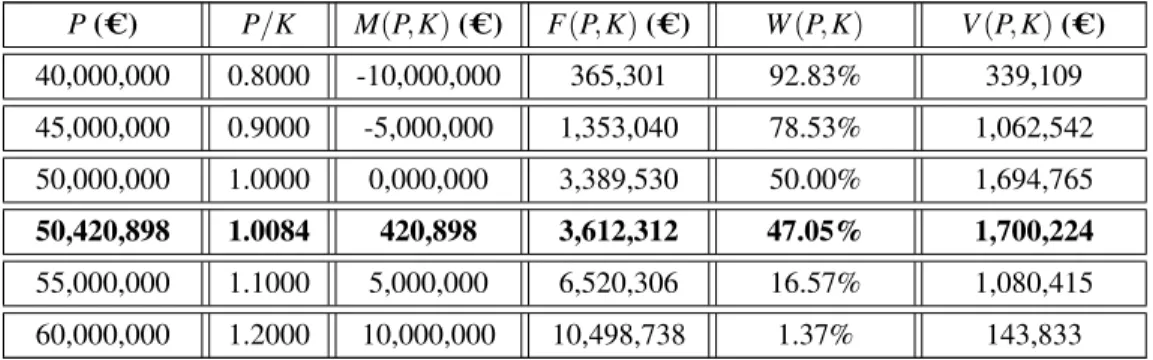
Table 2.3: different results for the option value, considering different price levels
(for: K = C 50,000,000; b = ln (1/0.5); n = 10; σ = 0.25; r =0.01; T − t = 0.5 years) P( C) P/K M(P, K) ( C) F(P, K) ( C) W(P, K) V(P, K) ( C) 40,000,000 0.8000 -10,000,000 365,301 92.83% 339,109 45,000,000 0.9000 -5,000,000 1,353,040 78.53% 1,062,542 50,000,000 1.0000 0,000,000 3,389,530 50.00% 1,694,765 50,420,898 1.0084 420,898 3,612,312 47.05% 1,700,224 55,000,000 1.1000 5,000,000 6,520,306 16.57% 1,080,415 60,000,000 1.2000 10,000,000 10,498,738 1.37% 143,833
The results included in Table 2.3 demonstrate that, the higher the value of the “underlying asset”, the higher the value of F(P, K) (the value of the option to sign the contract increases in response to the presence of higher bid prices) and the lower the value of W (P, K), since this probability decreases as the bid price (or mark-up bid) assumes greater values. This combined effect - reflecting opposite responses to variations in the bid price - makes V (P, K) increase until its maximum value is reached: C 1, 700, 224. To this maximum value of the option to invest weighted by the probability of winning the bid, V (P, K) corresponds the optimal