EUROPEAN ORGANIZATION FOR NUCLEAR RESEARCH (CERN)
CERN-PH-EP/2015-332 2016/05/03
CMS-EXO-14-010
Search for massive WH resonances decaying into the
`
ν
bb
final state at
√
s
=
8 TeV
The CMS Collaboration
∗Abstract
A search for a massive resonance W0 decaying into a W and a Higgs boson in the
`νbb (` = e, µ) final state is presented. Results are based on data corresponding
to an integrated luminosity of 19.7 fb−1 of proton-proton collisions at √s = 8 TeV, collected using the CMS detector at the LHC. For a high-mass (&1 TeV) resonance, the two bottom quarks coming from the Higgs boson decay are reconstructed as a single jet, which can be tagged by placing requirements on its substructure and flavour. Exclusion limits at 95% confidence level are set on the production cross section of a narrow resonance decaying into WH, as a function of its mass. In the context of a little Higgs model, a lower limit on the W0 mass of 1.4 TeV is set. In a heavy vector triplet model that mimics the properties of composite Higgs models, a lower limit on the W0mass of 1.5 TeV is set. In the context of this model, the results are combined with related searches to obtain a lower limit on the W0mass of 1.8 TeV, the most restrictive to date for decays to a pair of standard model bosons.
Published in the European Physical Journal C as doi:10.1140/epjc/s10052-016-4067-z.
c
2016 CERN for the benefit of the CMS Collaboration. CC-BY-3.0 license
∗See Appendix A for the list of collaboration members
1
1
Introduction
This paper presents a search for massive resonances decaying into a W and a standard model (SM) Higgs boson (H) [1–4] in the`νb ¯b (` =e, µ) final state. Such processes are distinctive
fea-tures of several extensions of the SM such as composite Higgs [5–7], SU(5)/SO(5) Littlest Higgs (LH) [8–11], technicolor [12, 13], and left-right symmetric models [14]. These models provide solutions to the hierarchy problem and predict new particles including additional gauge bosons such as a heavy W0. The W0in these models can have large branching fractions to WH and WZ, while the decays to fermions can be suppressed. The recently proposed heavy vector triplet (HVT) model [15] generalizes a large class of specific models that predict new heavy spin-1 vector bosons. In this model, the resonance is described by a simplified Lagrangian in terms of a small number of parameters representing its mass and couplings to SM bosons and fermions. For a W0with SM couplings to fermions and thus reduced decay branching ratio to SM bosons, the most stringent limits on production cross sections are reported in searches with leptonic final states [16, 17]. The current lower limit on the W0 mass is 3.3 TeV. In the same context, searches for a W0 decaying into a pair of SM vector bosons (WZ) [18–21] provide a lower mass limit of 1.7 TeV. In the context of a HVT model with reduced couplings to fermions (HVT model B), the most stringent limit of 1.7 TeV on the W0/Z0 mass is set by a search for W0/Z0 →WH/ZH→q ¯qb ¯b [22]. The same model is used to interpret the results of a search for W0/Z0 →WH/ZH→ `ν/``/νν+b ¯b [23]. A lower limit on the W0 mass of 1.5 TeV is set in
the same final state reported in Ref. [23]. Finally, a specific search for Z0 →ZH→q ¯qτ+τ−was
reported in Ref. [24] and interpreted in the context of the same HVT model B.
This analysis is based on proton-proton collision data at√s = 8 TeV collected by the CMS ex-periment at the CERN LHC during 2012, corresponding to an integrated luminosity of 19.7 fb−1. The signal considered is the production of a resonance with mass above 0.8 TeV decaying into WH, where the Higgs boson decays into a bottom quark-antiquark pair and the W boson de-cays into a charged lepton and a neutrino (Fig. 1). It is assumed that the resonance is narrow, i.e. that its intrinsic width is much smaller than the experimental resolution.
Figure 1: Production of a resonance decaying into WH.
The search strategy is closely related to the search for high mass WW resonances in the`νq ¯q
final state, described in Ref. [25], with the addition of b tagging techniques. We search for res-onances in the invariant mass of the WH system on top of a smoothly falling background dis-tribution, where the background mainly comprises events involving pair produced top quarks (tt) or a W boson produced in association with jets (W+jets). For the resonance mass range considered, the two quarks from the Higgs boson decay would be separated by a small angle,
2 3 Simulated samples
resulting in the detection of a single jet after hadronization. This jet is tagged as coming from a Higgs boson through the estimation of its invariant mass, application of jet substructure tech-niques [26], and use of specialized b tagging techtech-niques for high transverse momentum (pT)
Higgs bosons [27].
The results of this analysis are also combined with two previous results [22, 24] to obtain a further improvement in sensitivity.
2
CMS detector
The central feature of the CMS apparatus is a superconducting solenoid of 6 m internal diam-eter, providing a field of 3.8 T. Within the field volume are a silicon pixel and strip tracker, a crystal electromagnetic calorimeter (ECAL), and a brass and scintillator hadronic calorimeter (HCAL). The CMS tracker consists of 1440 silicon pixel and 15 148 silicon strip detector modules covering a pseudorapidity range of|η| <2.5. The ECAL consists of nearly 76 000 lead tungstate
crystals, which provide coverage of|η| <1.48 in the central barrel region and 1.48< |η| <3.00
in the two forward endcap regions. The HCAL consists of a sampling calorimeter [28], which utilizes alternating layers of brass as an absorber and plastic scintillator as an active material, covering the range|η| <3, and is extended to|η| <5 by a forward hadron calorimeter. Muons
are measured in the range|η| < 2.4 with detection planes which employ three technologies:
drift tubes, cathode strip chambers, and resistive-plate chambers. The muon trigger combines the information from the three sub-detectors with a coverage up to|η| <2.1. A more detailed
description of the CMS detector, together with a definition of the coordinate system used and the relevant kinematic variables, can be found in Ref. [28].
3
Simulated samples
For the modelling of the background we use the MADGRAPHv5.1.3.30 [29] event generator to
simulate the production of W boson and Drell–Yan events in association with jets, thePOWHEG
1.0 r1380 [30–35] package to generate tt and single top quark events, and PYTHIA v6.424 [36] for diboson (WW, WZ, and ZZ) processes. All simulated event samples are generated using the CTEQ6L1 [37] parton distribution functions (PDF) set, except for thePOWHEG tt sample, for which the CT10 PDF set [38] is used. All the samples are then processed further byPYTHIA, using the Z2* tune [39, 40] for simulation of parton showering and subsequent hadronization, and for simulation of the underlying event. The passage of the particles through the CMS de-tector is simulated using the GEANT4 package [41]. All simulated background samples are
normalized to the integrated luminosity of the recorded data, using inclusive cross sections de-termined at next-to-leading order, or next-to-next-to-leading order when available, calculated withMCFMv6.6 [42–45] andFEWZv3.1 [46], except for the tt sample, for which TOP++ v2.0 [47] is used.
To simulate the signature of interest, we use a model of a generic narrow spin-1 W0 resonance implemented with MADGRAPH. We verified that the kinematic distributions agree with those
predicted by implementations of the LH, composite Higgs and HVT models in MADGRAPH.
The resonance width differs in the three models, but in each case it is found to be negligible with respect to the experimental resolution. More details on the parameters used for interpretation of the models are given in Section 8.
Extra proton-proton interactions are combined with the generated events before detector sim-ulation to match the observed distribution of the number of additional interactions per bunch
3
crossing (pileup). The simulated samples are also corrected for observed differences between data and simulation in the efficiencies of the lepton trigger [16], the lepton identification/isolation [16], and the selection criteria identifying jets originating from hadronization of bottom quarks (b-tagged jets) [27].
4
Reconstruction and selection of events
4.1 Trigger and basic event selectionCandidate events are selected during data taking using single-lepton triggers, which require either one electron or one muon without isolation requirements. For electrons the minimum transverse momentum pT measured at the high level trigger is 80 GeV, while for muons the pT
must be greater than 40 GeV.
After trigger selection, all events are required to have at least one primary-event vertex re-constructed within a 24 cm window along the beam axis, with a transverse distance from the nominal pp interaction region of less than 2 cm [48]. If more than one identified vertex passes these requirements, the primary-event vertex is chosen as the one with the highest sum of p2T over its constituent tracks.
Individual particle candidates are reconstructed and identified using the CMS particle-flow (PF) algorithm [49, 50], by combining information from all subdetector systems. The recon-structed PF candidates are each assigned to one of the five candidate categories: electrons, muons, photons, charged hadrons, and neutral hadrons.
4.2 Lepton reconstruction and selection
Electron candidates are reconstructed by clustering the energy deposits in the ECAL and then matching the clusters with reconstructed tracks [51]. In order to suppress the multijet back-ground, electron candidates must pass quality criteria tuned for high-pT objects and an
iso-lation selection [52]. The total scalar sum of the pT over all the tracks in a cone of radius
∆R = √(∆η)2+ (∆φ)2 = 0.3 around the electron direction, excluding tracks within an
in-ner cone of∆R = 0.04 to remove the contribution from the electron itself, must be less than 5 GeV. A calorimetric isolation parameter is calculated by summing the energies of reconstructed deposits in both the ECAL and HCAL, not associated with the electron itself, within a cone of radius∆R= 0.3 around the electron. The veto threshold for this isolation parameter depends on the electron kinematic quantities and the average amount of additional energy coming from pileup interactions, calculated for each event. The electron candidates are required to have pT > 90 GeV and|η| < 1.44 or 1.57< |η| < 2.5, thus excluding the transition region between
ECAL barrel and endcaps.
Muons are reconstructed with a global fit using both the tracker and muon systems [53]. An isolation requirement is applied in order to suppress the background from multijet events in which muons are produced in the semileptonic decay of B hadrons. A cone of radius∆R=0.3 is constructed around the muon direction. Muon isolation requires that the scalar pTsum over
all tracks originating from the interaction vertex within the cone, excluding the muon itself, is less than 10% of the pTof the muon. The muon candidates are required to have pT > 50 GeV
and|η| <2.1 in each selected event.
Events are required to contain exactly one lepton candidate (electron or muon). That is, events are rejected if they contain a second lepton candidate with pT > 35 GeV (electrons) or pT >
4 4 Reconstruction and selection of events
4.3 Jets and missing transverse momentum reconstruction
Hadronic jets are identified by clustering PF candidates, using the FASTJET v3.0.1 software package [54]. In the jet-clustering procedure, charged PF candiates associated with pileup ver-tices are excluded, to reduce contamination from pileup. In order to identify a Higgs boson decaying into bottom quarks, jets are clustered using the Cambridge–Aachen algorithm [55] with a distance parameter of 0.8 (“CA8 jets”). Only the highest pT CA8 jet is used. Jets in the
event are also identified using the anti-kTjet-clustering algorithm [56] with a distance
param-eter of 0.5 (“AK5 jets”). AK5 jets are required to be separated from the CA8 jet by ∆R > 0.8. An event-by-event correction based on the projected area of the jet on the front face of the cal-orimeter is used to remove the extra energy deposited in jets by neutral particles coming from pileup. Furthermore, jet energy corrections are applied, based on measurements in dijet and photon+jet events in data [57]. Additional quality criteria are applied to the jets in order to remove spurious jet-like features originating from calorimeter noise [58]. The CA8 (AK5) jets are required to be separated from the selected electron or muon candidate by∆R > 0.8 (0.3). Only jets with pT > 30 GeV and|η| < 2.4 are allowed in the subsequent steps of the analysis.
Furthermore, CA8 jets are not used in the analysis if their pseudorapidity falls in the region 1.0 < |η| < 1.8, thus overlapping the barrel-endcap transition region of the silicon tracker.
In that region, ’noise’ can arise when the tracking algorithm reconstructs many fake displaced tracks associated with the jet. The simulation does not sufficiently describe the full material budget of the tracking detector in that region, thus it does not accurately describe this effect. Without this requirement, a bias can be introduced in the b tagging, jet substructure and miss-ing transverse momentum information, makmiss-ing this analysis systematically prone to that noise. The probability of signal events satisfying the requirement that the pseudorapidity of the CA8 jet falls outside the region 1.0< |η| <1.8 is 80% (92%) for a resonance mass of 1.0 (2.5) TeV.
A b tagging algorithm, known as the combined secondary vertex algorithm [27, 59], is applied to reconstructed AK5 jets to identify whether they originate from bottom quarks. This method allows the identification and rejection of the tt events as described in Section 4.6. The chosen algorithm working point provides a misidentification rate for light-parton jets of∼1% and an efficiency of∼70% [27]. The simulated events are reweighted event-by-event with the ratio of the b tagging efficiency in data and simulation, determined in a sample enriched with b-jets. The average value of the correction factor is 0.95. The same b tagging algorithm is also used to identify whether the CA8 jet comes from a Higgs boson decaying into bottom quarks, as described in Section 4.5.
The missing transverse momentum pmissT is defined as the magnitude of the projection on the plane perpendicular to the beams of the negative vector sum of the momenta of all the recon-structed particles in an event. The raw pmissT value is modified to account for corrections to the energy-momentum scale of all the reconstructed AK5 jets in the event. More details on the pmiss
T performance in CMS can be found in Refs. [60, 61]. A requirement of pmissT >80(40)GeV
is applied for the electron (muon) channel. The higher threshold for the electron channel is motivated by the higher contribution from the multijet background expected in the low-pmissT range due to jets misidentified as electrons. The background is expected to be negligible in the muon channel, for which a lower pmissT threshold can be used to preserve a higher efficiency for a low-mass signal.
4.4 The W
→ `
ν reconstruction and identificationThe identified electron or muon is associated with the W → `νcandidate. The pT of the
un-detected neutrino is assumed to be equal to the pmiss
4.5 TheH→bb identification using jet substructure and b tagging 5
neutrino momentum is calculated following a method used originally for the reconstruction of the invariant mass of the top quark as described in Ref. [62]. The method aims to solve a quadratic equation that makes use of the known W boson mass. Kinematic ambiguities in the solution of the equation are resolved as in Ref. [62]. The four-momentum of the neutrino is used to build the four-momentum of the W→ `νcandidate.
4.5 The H
→
bb identification using jet substructure and b taggingThe CA8 jets are used to reconstruct the jet candidates from decays of Lorentz-boosted Higgs boson to bottom quarks. We exploit two techniques to discriminate against quark and gluon jets from the multijet background, including the requirement that the reconstructed jet mass be close to the Higgs boson mass, and b tagging methods that discriminate jets originating from the b quarks from those originating from lighter quarks or gluons.
First, we apply a jet-grooming technique [26, 63] to re-cluster the jet constituents, while ap-plying additional requirements to remove possible contamination from soft QCD radiation or pileup. Different jet-grooming algorithms have been explored at CMS, and their performance on jets in multijet processes has been studied in detail [63]. In this analysis, we use the jet pruning algorithm [64, 65], which re-clusters each jet starting from all its original constituents using the CA algorithm iteratively, while discarding soft and large-angle recombinations at each step. The performance of the algorithm depends on the two parameters, zcut = 0.1 and
Dcut =mjet/pjetT , which define the maximum allowed hardness and the angle of the
recombina-tions in the clustering algorithm, respectively. A jet is considered as an H-tagged jet candidate if its pruned mass, mjet, computed from the sum of the four-momenta of the constituents
sur-viving the pruning, falls in the range 110<mjet <135 GeV. The mjetwindow is the result of an
optimization based on signal sensitivity and on the constraints due to the higher bounds of the signal regions of other diboson analyses [25].
The simulation modelling of the pruned mass measurement for merged jets from heavy bosons has been checked using merged W →qq0 decays in tt events with a`+jets topology [26]. The data are compared with tt events generated with MADGRAPH, interfaced toPYTHIAfor parton showering. The differences between recorded and simulated event samples in the pruned jet mass scale and resolution are found to be up to 1.7% and 11%, respectively. In addition, the modelling of bottom quark fragmentation is checked through reconstruction of the top quark mass in these tt events [66].
To discriminate between quark and gluon jets, on one hand, and a Higgs-initiated jet, on the other, formed by the hadronization of two bottom quarks, we use a H tagging technique [27]. This procedure splits the candidate H-jet into two sub-jets by reversing the last step of the CA8 pruning recombination algorithm. Depending on the angular separation ∆R of the two sub-jets, different b tagging discriminators are used to tag the H-jet candidate. If∆R > 0.3, then the b tagging algorithm is applied to both of the individual sub-jets of the CA8 jet; otherwise, it is applied to the whole CA8 jet. The chosen algorithm working point provides a misidentifi-cation rate of 10% and an efficiency of 80%. The ratio of the b tagging efficiency between data and simulation, in a sample enriched with b-jets from gluon splitting by requiring two muons within the CA8 jet, is used to reweight the simulated events.
4.6 Final event selection and categorization
After reconstructing the W and Higgs bosons, we apply the final selections used for the search. Both the W and Higgs boson candidates must have a pT greater than 200 GeV. In addition, we
6 5 Modelling of background and signal
back-to-back, since they tend to be isotropically distributed for background events. In partic-ular, the ∆R distance between the lepton and the H-tagged jet must be greater than π/2, the azimuthal angular separation between the pmissT and the H-tagged jet must be greater than 2.0 radians, and the azimuthal angular separation between the W → `ν and H-tagged jet
can-didates must be greater than 2.0 radians. To further reduce the level of the tt background, events with one or more reconstructed AK5 jets, not overlapping with the CA8 H-tagged jet candidate as described previously in Section 4.3, are analyzed. If one or more of the AK5 jets is b-tagged, the event is rejected. Furthermore, a leptonically decaying top quark candidate mass m`topis reconstructed from the lepton, pmissT , and the closest AK5 jet to the lepton using the method described in Ref. [62]. A hadronically decaying top quark candidate mass mhtop is reconstructed from the CA8 H-tagged jet candidate and the closest AK5 jet. Events with 120<m`top <240 GeV or 160<mhtop <280 GeV are rejected. The chosen windows around the top quark mass are the result of an optimization carried out in this analysis, taking into account the asymmetric tails at larger values due to combinatorial background. If several distinct WH resonance candidates are present in the same event, only the candidate with the highest-pT
H-tagged jet is kept for further analysis. The invariant mass of the WH resonance (MWH) is
required to be at least 0.7 TeV. The signal efficiency for the full event selection ranges between
∼3% and∼9%, depending on the resonance mass.
5
Modelling of background and signal
5.1 Background estimationAfter the full event selection, the two dominant remaining backgrounds are expected to come from W+jets and tt events. Backgrounds from tt, single top quark, and diboson production are estimated using simulated samples after applying correction factors derived from control samples in data. For the W+jets background estimation, a procedure based on data has been developed to determine both the normalization and the MWHshape.
For the W+jets normalization estimate, a signal-depleted control region is defined outside the mjetmass window described in Section 4.5. A lower sideband region is defined in the mjetrange
[40, 110] GeV as well as an upper sideband in the range [135, 150] GeV. The overall normaliza-tion of the W+jets background in the signal region is determined from the likelihood of the sum of backgrounds fit to the mjetdistribution in both sidebands of the observed data. In this
approach, simulated events are replaced by an analytical function, which has been determined individually for each background process. Figure 2 shows the result of this fit procedure, where all selections are applied except the final mjetsignal window requirement. The inclusive W+jets
background is predicted from a fit excluding the signal region (between the vertical dashed lines), while the other backgrounds are estimated from simulation.
The shape of the W+jets background as a function of MWHin the signal region is estimated
us-ing the lower sideband region of the mjetdistribution. Correlations needed to extrapolate from
the sideband to the signal region are determined from simulation through an extrapolation function defined as:
αMC(MWH) =
FMC,SRW+jets(MWH)
FMC,SBW+jets(MWH)
, (1)
where FMC,SRW+jetsand FMC,SBW+jetsare the probability density functions determined from the MWH
5.1 Background estimation 7 [GeV] jet m 40 60 80 100 120 140 data σ Data-Fit -2 0 2 40 60 80 100 120 140 Events / 5 GeV 5 10 15 20 25 30 35 Data (eν) W+jets Top WW/WZ/ZZ Uncertainty (8 TeV) -1 19.7 fb CMS [GeV] jet m 40 60 80 100 120 140 data σ Data-Fit -2 0 2 40 60 80 100 120 140 Events / 5 GeV 10 20 30 40 50 60 Data (µν) W+jets Top WW/WZ/ZZ Uncertainty (8 TeV) -1 19.7 fb CMS
Figure 2: Distributions of the pruned jet mass, mjet, in the electron (left) and muon (right)
channels. The signal region lies between the dashed vertical lines. The hatched region indicates the statistical uncertainty of the fit. At the bottom of each plot, the bin-by-bin fit residuals,
(Data−Fit)/σdata, are shown.
In order to estimate the W+jets contribution FDATA,SBW+jets in the control region of the data the other backgrounds are subtracted from the observed MWHdistribution in the lower sideband region.
The shape of the W+jets background distribution in the signal region is obtained by scaling FDATA,SBW+jets according to αMC. The final prediction of the background contribution in the signal
region, NSRBKGD, is given by NSRBKGD(MWH) =CW +jets SR F W+jets DATA,SB(MWH)αMC(MWH) +
∑
k CSRk FMC,SRk (MWH), (2)where the index k runs over the list of minor backgrounds, and CSRW+jets and CSRk represent the normalizations of the yields of the dominant W+jets background and of the different minor background contributions. The CSRW+jets parameter is determined from the fit to the mjet
distri-bution as described above, while each CSRk is determined from simulation. The ratio αMC
ac-counts for the small kinematic differences between signal and sideband regions, and is largely independent of the assumptions on the overall cross section. The validity and robustness of this method have been studied in data using a lower mjetsideband of [40, 80] GeV to predict an
alternate signal region with mjet in the range [80, 110] GeV. Both the normalization and shape
of the W+jets background are successfully estimated for the alternate signal region. This al-ternate signal region differs from the signal region of the search for WW or WZ resonances in Ref. [25] as b tagging is applied to the CA8 jet. We are therefore able to evaluate the potential WW and WZ signal contamination in the alternate signal region and find less than 5% signal contamination, assuming a signal cross section corresponding to the exclusion limit for a WW resonance from Ref. [25]. The MWH distribution of the background in the signal and lower
sideband regions is described analytically by a function defined as f(x)∝ exp[−x/(c0+c1x)],
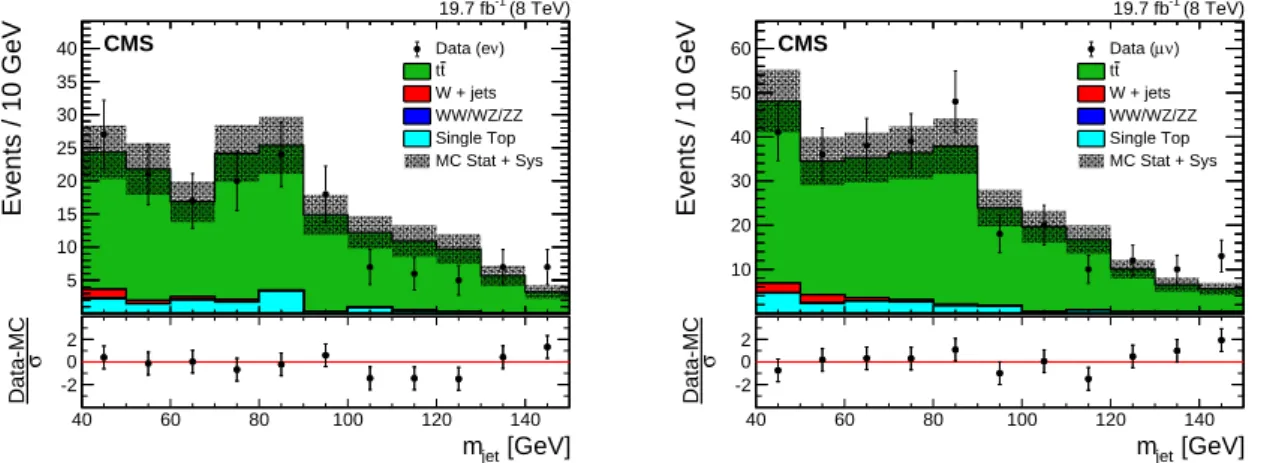
which is found to describe the simulation well. Alternative fit functions have been studied but in all cases the background shapes agree with that of the default function within uncertainties. For the tt background estimate, a control sample is selected by applying all analysis require-ments, except that the b-tagged jet veto is inverted, the veto on the top quark mass is dropped, and the mjetrequirement is removed. The data are compared with the predictions from
simula-tion and good agreement is found. The pruned jet mass distribusimula-tion in the top quark enriched control sample is shown in Fig. 3. The pruned jet mass distribution shows a small peak due to isolated W boson decays into hadrons, along with a smoothly varying combinatorial
com-8 6 Systematic uncertainties
ponent mainly due to events in which the extra b-tagged jet from the top quark decay is in the proximity of the W boson. The difference in normalization between data and simulation is found to be 4.6±5.6%, where the quoted uncertainty is only statistical. This normalization difference is applied to correct the normalization of tt background in the signal region. The relative uncertainty of 5.6% is used to quantify the uncertainty in the tt and single top quark background normalization, as described in Section 6.1.
40 60 80 100 120 140 Events / 10 GeV 5 10 15 20 25 30 35 40 Data (eν) t t W + jets WW/WZ/ZZ Single Top MC Stat + Sys (8 TeV) -1 19.7 fb CMS [GeV] jet m 40 60 80 100 120 140 σ Data-MC -2 0 2 40 60 80 100 120 140 Events / 10 GeV 10 20 30 40 50 60 Data (µν) t t W + jets WW/WZ/ZZ Single Top MC Stat + Sys (8 TeV) -1 19.7 fb CMS [GeV] jet m 40 60 80 100 120 140 σ Data-MC -2 0 2
Figure 3: Distributions of mjetin the top quark enriched control sample in the electron (left) and
muon (right) channels. The hatched region indicates the overall uncertainty in the background. In the lower panels, the bin-by-bin residuals,(Data−MC)/σ are shown, where σ is the sum in quadrature of the statistical uncertainty of the data, the simulation, and the systematic uncer-tainty in the tt background.
5.2 Modelling of the signal mass distribution
The shape of the reconstructed signal mass distribution is extracted from the simulated signal samples. In the final analysis of the MWHspectrum, the statistical signal sensitivity depends on
an accurate description of the signal shape. The signal shape is parametrized with a double-sided Crystal Ball function (i.e. a Gaussian core with power-law tails on both sides) [67] to describe the CMS detector resolution. Figure 4 shows an example of this parametrization for a W0 mass of 1.5 TeV. To take into account differences between the electron and muon pT
res-olutions at high pT, the signal mass distribution is parametrized separately for events with
electrons and muons. The resolution of the reconstructed MWH is given by the width of the
Gaussian core and is found to be 4–6%.
6
Systematic uncertainties
6.1 Systematic uncertainties in the background estimation
Uncertainties in the estimation of the background affect both the normalization and the shape of the MWH distribution. The systematic uncertainty in the W+jets background yield is
dom-inated by the statistical uncertainty associated with the number of events in data in the mjet
sideband regions, and it is found to be about 59% (42%) in the electron (muon) channel. The systematic uncertainty in the tt normalization comes from the data-to-simulation ratio derived in the top-quark-enriched control sample (5.6%) as described in Section 5.1. The systematic un-certainties in the WW, WZ, and ZZ inclusive cross sections are assigned to be 10%, taken from the relative difference in the mean value between the CMS WW cross section measurement at
√
6.2 Systematic uncertainties in the signal prediction 9
Systematic uncertainties in the W+jets background shape are estimated from the covariance matrix of the fit to the extrapolated data sideband and from the uncertainties in the modelling of αMC(MWH). They are driven by the available data in the sidebands and the number of events
generated for the simulation of the W+jets background, respectively. These uncertainties are shown in Fig. 4, and they are found to be about 30% (120%) at MWH ≈ 1 TeV (1.8 TeV). The
es-timation of the systematic uncertainty in the shape of the tt background takes into account the following contributions: the statistical uncertainty associated with the simulated event sam-ple, the choices of regularization/factorization scales (varied up and down by a factor of 2), the matching scales in the MADGRAPHsimulation, and an observed difference between MAD
-GRAPHandPOWHEGsimulations.
Systematic effects from rare noise events identified in the tracker overlap region were specif-ically studied in the context of the acceptance requirement introduced for H-jet candidates (|η| < 1.0 or|η| > 1.8) as described in Section 4. Those studies conclude that any residual
noise effects following the imposition of this requirement are negligible. No additional source of systematic uncertainty is taken into account for the background predictions.
6.2 Systematic uncertainties in the signal prediction
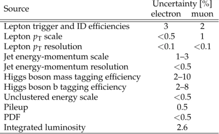
Systematic uncertainties in the signal prediction affect both the signal efficiency and the MWH
shape. The primary uncertainties in signal yields are summarized in Table 1 and described below.
The systematic uncertainties in the signal efficiency due to the electron energy (E) and muon pT scales are evaluated by varying the lepton E or pT within one standard deviation of the
corresponding uncertainty [51, 53]; the uncertainties due to the electron E and muon pT
resolu-tions are estimated applying a pTand E smearing, respectively. In this process, variations in the
lepton E or pTare propagated consistently to the pmissT vector. We also take into account the
sys-tematic uncertainties affecting the observed-to-simulated scale factors for the efficiencies of the lepton trigger, identification and isolation requirements. These efficiencies are derived using a specialized tag-and-probe analysis with Z→ `+`−events [69], and the uncertainty in the ratio
of the efficiencies is taken as the systematic uncertainty. The uncertainties in the efficiencies of the electron (muon) trigger and the electron (muon) identification with isolation are 3% (3%) and 3% (4%), respectively.
The signal efficiency is also affected by the uncertainties in the jet energy-momentum scale and resolution. The jet energy-momentum scale and resolution are varied within their pT- and
η-dependent uncertainties [57] to estimate their impact on the signal efficiency. The variations are also propagated consistently to the pmiss
T vector.
The momentum scale uncertainty of particles that are not identified as leptons or clustered in jets (‘unclustered energy-momentum’) is found to introduce an uncertainty of less than 0.5% in the signal efficiency.
We also include systematic uncertainties in the signal efficiency due to uncertainties in data-to-simulation scale factors for the pruned jet mass tagging, derived from the top quark enriched control sample [26] and b-tagged jet identification efficiencies [27]. These sources introduce a systematic uncertainty in the mass tagging and b tagging of the Higgs boson of 2–10% and 2–8%, respectively, depending on the signal mass.
The systematic uncertainty due to the modelling of pileup is estimated by reweighting the signal simulation samples such that the distribution of the number of interactions per bunch crossing is shifted according to the uncertainty in the inelastic proton-proton cross section [70,
10 7 Results
71].
The impact of the proton PDF uncertainties on the signal efficiency is evaluated with the PDF4LHC prescription [72, 73], using the MSTW2008 [74] and NNPDF2.1 [75] PDF sets. The uncertainty in the integrated luminosity is 2.6% [76].
Table 1: Summary of the systematic uncertainties in the signal yield, relative to the expected number of events.
Source Uncertainty [%]
electron muon Lepton trigger and ID efficiencies 3 2
Lepton pTscale <0.5 1
Lepton pTresolution <0.1 <0.1
Jet energy-momentum scale 1–3 Jet energy-momentum resolution <0.5 Higgs boson mass tagging efficiency 2–10 Higgs boson b tagging efficiency 2–8 Unclustered energy scale <0.5
Pileup 0.5
PDF <0.5
Integrated luminosity 2.6
In addition to systematic uncertainties in the signal efficiency discussed above, we consider un-certainties in the signal resonance peak position and width. The systematic effects that could change the signal shape are the uncertainties due to the pT/energy-momentum scale and
res-olution of electrons, muons, jets, and the unclustered energy-momentum scale. For each of these sources of experimental uncertainty, the energy-momentum of the lepton and jets, as well as the corresponding pmiss
T vector, are varied (or smeared) by their relative uncertainties.
The uncertainty in the peak position of the signal is estimated to be less than 1%. The jet energy-momentum scale and resolution introduce a relative uncertainty of about 3% in the sig-nal width. The unclustered energy-momentum scale introduces an uncertainty in the sigsig-nal width of 1% at lower resonance masses (<1.5 TeV), and of 3% at higher masses.
7
Results
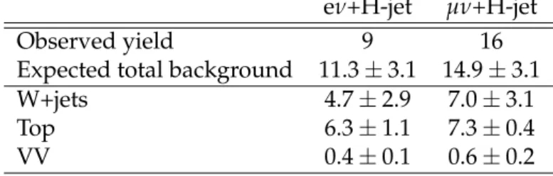
The predicted number of background events in the signal region after the inclusion of all back-grounds is summarized in Table 2 and compared with observations. The yields are quoted in the range 0.7 < MWH < 3 TeV. The expected background is derived with the sideband
pro-cedure. The uncertainties in the background prediction from data are statistical in nature, as they depend on the number of events in the sideband region. The muon channel has more expected background events than the electron channel owing to the lower pmissT requirement on the muon and its worse mass resolution at high pT.
Figure 4 shows the MWHspectra after all selection criteria have been applied. The highest mass
event is in the electron category and has MWH≈1.9 TeV. The observed data and the predicted
background in the muon channel agree. In the electron channel, an excess of three events is observed with MWH>1.8 TeV, where about 0.3 events are expected, while in the muon channel
11
Table 2: Observed and expected yields in the signal region together with statistical uncertain-ties.
eν+H-jet µν+H-jet
Observed yield 9 16
Expected total background 11.3±3.1 14.9±3.1 W+jets 4.7±2.9 7.0±3.1 Top 6.3±1.1 7.3±0.4 VV 0.4±0.1 0.6±0.2 [TeV] WH M 0.8 1 1.2 1.4 1.6 1.8 2 2.2 2.4 Events / 0.1 TeV -2 10 -1 10 1 10 2 10 ) ν Data (e W' HVT B (gv=3) Uncertainty W+jets Top WW/WZ/ZZ (8 TeV) -1 19.7 fb CMS [TeV] WH M 0.8 1 1.2 1.4 1.6 1.8 2 2.2 2.4 Events / 0.1 TeV -2 10 -1 10 1 10 2 10 ) ν µ Data ( W' HVT B (gv=3) Uncertainty W+jets Top WW/WZ/ZZ (8 TeV) -1 19.7 fb CMS
Figure 4: Final distributions in MWHfor data and expected backgrounds for electron (left) and
muon (right) categories. The 68% error bars for Poisson event counts are obtained from the Neyman construction [77]. The hatched region indicates the statistical uncertainty of the fit combined with the systematical uncertainty in the shape. This figure also shows a hypothetical W0signal with mass of 1.5 TeV, normalized to the cross section predicted by the HVT model B with parameter gV=3 as described in Section 8.2.
12 8 Statistical and model interpretation
8
Statistical and model interpretation
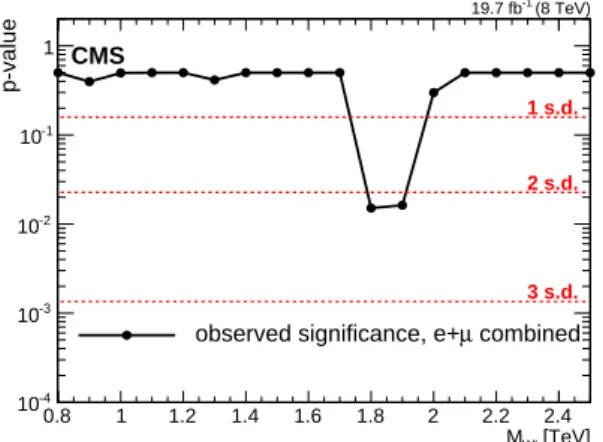
8.1 Significance of the dataA comparison between the MWH distribution observed in data and the largely data-driven
background prediction is used to test for the presence of a resonance decaying into WH. The statistical test is performed based on a profile likelihood discriminant that describes an un-binned shape analysis. Systematic uncertainties in the signal and background yields are treated as nuisance parameters and profiled in the statistical interpretation using log-normal priors. We evaluate the local significance of the observations in the context of the described test, under the assumptions of a narrow resonance decaying into the WH final state and lepton universal-ity for the W boson decay, by combining the two event categories. Correlations arising from the uncertainties common to both channels are taken into account. The result is shown in Fig. 5. The highest local significance of 2.2 standard deviations is found for a resonance mass of 1.8 TeV, driven by the excess in the electron channel described in Section 7. The corresponding local significance for a resonance of 1.8 TeV in the electron channel is 2.9 standard deviations, while in the muon channel there is no significance. Taking into account the look-elsewhere effect [78], a local significance of 2.9 standard deviations translates into a global significance of about 1.9 standard deviations searching for resonances over the full mass range 0.8–2.5 TeV and across two channels. We conclude that the results are thus statistically compatible with the SM expectation within 2 standard deviations.
[TeV] W' M 0.8 1 1.2 1.4 1.6 1.8 2 2.2 2.4 p-value -4 10 -3 10 -2 10 -1 10 1 (8 TeV) -1 19.7 fb CMS combined µ observed significance, e+ 1 s.d. 2 s.d. 3 s.d.
Figure 5: Local p-value of the combined electron and muon data as a function of the W0 boson mass, probing a narrow WH resonance.
8.2 Cross section limits
We set upper limits on the production cross section of a new resonance following the modified-frequentist CLsmethod [79, 80]. Exclusion limits can be set as a function of the W0boson mass,
under the narrow-width approximation. The results are interpreted in the HVT model B [15] which mimics the properties of composite Higgs scenarios, and in the context of the little Higgs model [8]. Typical parameter values for the HVT model B are
|cH| ≈ |cF| ≈1, gV≥3, (3)
where cHdescribes interactions involving the Higgs boson or longitudinally polarized SM
vec-tor bosons, cF describes the direct interactions of the W0 with fermions, and gV is the typical
strength of the new interaction. In this scenario, decays of the W0 boson into a diboson are dominant and the W0 →WH branching fraction is almost equal to that of the decay into WZ.
8.2 Cross section limits 13
The parameter points for this scenario are currently not well constrained from experiments [15] because of the suppressed fermionic couplings of the W0boson.
The following parameters are used for interpretation of the results: gV=3, cH= −1 and cF=1
in the HVT model B and cot 2θ = 2.3, cot θ = −0.20799 in the LH model, where θ is a mixing angle parameter that determines W0 couplings and that cot 2θ and cot θ can be directly related to cHand cF.
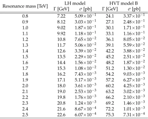
The intrinsic width and cross section for both models are listed in Table 3 for several resonance masses. The widths for the HVT model B are computed by means of Eqs. (2.25) and (2.31) in Ref. [15], while the cross sections were obtained using the online tools provided by the authors of Ref. [15]. The width is less than 5% for the following parameter values: 0.95 < gV < 3.76,
cH = −1, and cF = 1; gV < 3.9, cH = −1, and cF = 0; or gV < 7.8, cH = 0.5, and cF = 0. The
widths for the LH model have been computed by means of Eq. (15) in Ref. [81], and they are less than 5% for values of 0.084 < |cot θ| < 1.21. Hence, in both models we can consider the width to be negligible compared to the experimental resolution.
Table 3: Intrinsic total widths (Γ) and cross sections (σ) for the LH model and HVT model B for different resonance masses. The WH → `νbb branching fraction is not included in the
calculation.
Resonance mass [TeV] Γ [GeV]LH model HVT model B σ[pb] Γ [GeV] σ[pb] 0.8 7.22 5.09×10⁻¹ 24.1 3.37×10⁻¹ 0.9 8.12 3.03×10⁻¹ 27.1 2.48×10⁻¹ 1.0 9.02 1.87×10⁻¹ 30.1 1.71×10⁻¹ 1.1 9.92 1.18×10⁻¹ 33.1 1.16×10⁻¹ 1.2 10.8 7.65×10⁻² 36.1 8.05×10⁻² 1.3 11.7 5.06×10⁻² 39.1 5.59×10⁻² 1.4 12.6 3.39×10⁻² 42.2 3.88×10⁻² 1.5 13.5 2.29×10⁻² 45.2 2.51×10⁻² 1.6 14.4 1.56×10⁻² 48.2 1.87×10⁻² 1.7 15.3 1.08×10⁻² 51.2 1.30×10⁻² 1.8 16.2 7.43×10⁻³ 54.2 9.03×10⁻³ 1.9 17.1 5.17×10⁻³ 57.2 6.27×10⁻³ 2.0 18.0 3.61×10⁻³ 60.2 4.25×10⁻³ 2.1 19.0 2.53×10⁻³ 63.2 3.02×10⁻³ 2.2 19.8 1.76×10⁻³ 66.2 2.10×10⁻³ 2.3 20.8 1.24×10⁻³ 69.2 1.46×10⁻³ 2.4 21.6 8.67×10⁻⁴ 72.2 1.01×10⁻³ 2.5 22.6 6.07×10⁻⁴ 75.3 7.31×10⁻⁴
Figure 6 shows the expected and observed exclusion limits at 95% confidence level (CL) on the product of the W0 production cross section and the branching fraction of W0 → WH for the electron and muon channels separately, and for the combination of the two. For the combined channels, the observed and expected lower limits on the W0 mass are 1.4 TeV in the LH model and 1.5 TeV in the HVT model B. For the electron (muon) channel, the observed and expected lower limits on the W0mass are 1.2 (1.3) TeV in the LH model and 1.3 (1.3) TeV in the HVT model B.
14 8 Statistical and model interpretation [TeV] W' M 0.8 1 1.2 1.4 1.6 1.8 2 WH) [pb] → B(W' × σ -3 10 -2 10 -1 10 1 10 0.8 Observed 1 s.d. ± Expected 2 s.d. ± Expected HVT B(gv=3) LH (8 TeV) -1 19.7 fb CMS e channel [TeV] W' M 0.8 1 1.2 1.4 1.6 1.8 2 WH) [pb] → B(W' × σ -3 10 -2 10 -1 10 1 10 0.8 Observed 1 s.d. ± Expected 2 s.d. ± Expected HVT B(gv=3) LH (8 TeV) -1 19.7 fb CMS channel µ [TeV] W' M 0.8 1 1.2 1.4 1.6 1.8 2 WH) [pb] → B(W' × σ -3 10 -2 10 -1 10 1 10 0.8 Observed 1 s.d. ± Expected 2 s.d. ± Expected HVT B(gv=3) LH (8 TeV) -1 19.7 fb CMS combined µ e+
Figure 6: Observed (solid) and expected (dashed) upper limits at 95% CL on the product of the W0 production cross section and the branching fraction of W0 → WH for electron (upper left) and muon (upper right) channels, and the combination of the two channels (lower plot). The products of cross sections and branching fractions for W0 production in the LH and HVT models are overlaid.
8.3 Analysis combination 15
8.3 Analysis combination
The limits obtained in this analysis can be combined with two previous results [22, 24], setting limits on the sum of W0 →WH and Z0 →ZH production in the context of the HVT model. The search for W0/Z0 → WH/ZH → q0qbb/qqqqqq [22] reports limits in the context of the HVT model that can be directly used in the combination. However, while an asymptotic approxi-mation of the CLs procedure was used in the original paper, for the combination the limit is
re-evaluated with the CLsprocedure reported above. The search for Z0 →ZH→qqτ+τ−[24],
does not report limits in the context of a W0 resonance. However, since it is also sensitive to a signal from W0 → WH → q0qτ+τ−with an efficiency of about 5% less than for the Z0 signal,
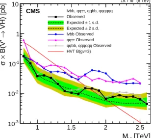
it was reinterpreted for the purpose of the combination. The results of the combination are shown in Fig. 7. The limit on the mass of the W0/Z0 is slightly improved to 1.8 TeV compared to the most stringent result reported by the W0/Z0 →WH/ZH→q0qbb/qqqqqq search.
[TeV] V' M 1 1.5 2 2.5 VH) [pb] → B(V' × σ -3 10 -2 10 -1 10 1 10 , qqbb, qqqqqq τ τ lvbb, qq Observed 1 s.d. ± Expected 2 s.d. ± Expected lvbb Observed Observed τ τ qq qqbb, qqqqqq Observed HVT B(gv=3) (8 TeV) -1 19.7 fb CMS lvbb, qqττ, qqbb, qqqqqq Observed 1 s.d. ± Expected 2 s.d. ± Expected lvbb Observed Observed τ τ qq qqbb, qqqqqq Observed HVT B(gv=3)
Figure 7: Observed (full rectangles) and expected (dashed line) combined upper limits at 95% CL on the sum of the W0and Z0production cross sections, weighted by their respective branch-ing fraction of W0 → WH and Z0 → ZH. The cross section for the production of a W0 and Z0 in the HVT model B, multiplied by its branching fraction for the relevant process, is overlaid. The observed limits of the three analyses entering the combination in the final states,`νbb (full
circle), qqτ+τ− [24] (full triangle pointing up), and qqbb/qqqqqq [22] (full triangle pointing
down), are overlaid.
In Fig. 8, a scan of the coupling parameters and the corresponding observed 95% CL exclusion contours in the HVT model from the combination of the analyses are shown. The parameters are defined as gVcH and g2cF/gV, related to the coupling strengths of the new resonance to
the Higgs boson and to fermions. The range of the scan is limited by the assumption that the new resonance is narrow. A contour is overlaid, representing the region where the theoretical width is larger than the experimental resolution of the searches, and hence where the narrow-resonance assumption is not satisfied. This contour is defined by a predicted narrow-resonance width of 7%, corresponding to the largest resonance mass resolution of the considered searches.
9
Summary
A search has been presented for new resonances decaying into WH, in which the W boson de-cays into`νwith` = e, µ and the Higgs boson decays to a pair of bottom quarks. Each event
16 9 Summary H c V g -3 -2 -1 0 1 2 3 V /gF c 2 g -1 -0.5 0 0.5 1 1.5 TeV 2 TeV 1 TeV =3) V B(g M exp σ ≈ > 7% M th Γ (8 TeV) -1 19.7 fb
CMS
Figure 8: Exclusion regions in the plane of the HVT-model couplings (gVcH, g2cF/gV) for three
resonance masses, 1, 1.5, and 2 TeV, where g denotes the weak gauge coupling. The point B of the benchmark model used in the analysis is also shown. The boundaries of the regions outside these lines are excluded by this search are indicated by the solid and dashed lines (region outside these lines is excluded). The areas indicated by the solid shading correspond to regions where the resonance width is predicted to be more than 7% of the resonance mass and the narrow-resonance assumption is not satisfied.
is reconstructed as a leptonic W boson candidate recoiling against a jet with mass compatible with the Higgs boson mass. A specialized b tagging method for Lorentz-boosted Higgs bosons is used to further reduce the background from multijet processes. No excess of events above the standard model prediction is observed in the muon channel, while an excess with a local significance of 2.9 standard deviations is observed in the electron channel near MWH≈1.8 TeV.
The results are statistically compatible with the standard model within 2 standard deviations. In the context of the little Higgs and the heavy vector triplet models, upper limits at 95% con-fidence level are set on the W0 production cross section in a range from 100 to 10 fb for masses between 0.8 and 2.5 TeV, respectively. Within the little Higgs model, a lower limit on the W0 mass of 1.4 TeV has been set. A heavy vector triplet model that mimics the properties of com-posite Higgs models has been excluded up to a W0 mass of 1.5 TeV. In this latter context, the results have been combined with related searches, improving the lower limit up to ≈1.8 TeV. This combined limit is the most restrictive to date for W0 decays to a pair of standard model bosons.
Acknowledgments
We congratulate our colleagues in the CERN accelerator departments for the excellent perfor-mance of the LHC and thank the technical and administrative staffs at CERN and at other CMS institutes for their contributions to the success of the CMS effort. In addition, we gratefully acknowledge the computing centres and personnel of the Worldwide LHC Computing Grid for delivering so effectively the computing infrastructure essential to our analyses. Finally, we acknowledge the enduring support for the construction and operation of the LHC and the CMS detector provided by the following funding agencies: BMWFW and FWF (Austria); FNRS and
References 17
FWO (Belgium); CNPq, CAPES, FAPERJ, and FAPESP (Brazil); MES (Bulgaria); CERN; CAS, MoST, and NSFC (China); COLCIENCIAS (Colombia); MSES and CSF (Croatia); RPF (Cyprus); MoER, ERC IUT and ERDF (Estonia); Academy of Finland, MEC, and HIP (Finland); CEA and CNRS/IN2P3 (France); BMBF, DFG, and HGF (Germany); GSRT (Greece); OTKA and NIH (Hungary); DAE and DST (India); IPM (Iran); SFI (Ireland); INFN (Italy); MSIP and NRF (Re-public of Korea); LAS (Lithuania); MOE and UM (Malaysia); CINVESTAV, CONACYT, SEP, and UASLP-FAI (Mexico); MBIE (New Zealand); PAEC (Pakistan); MSHE and NSC (Poland); FCT (Portugal); JINR (Dubna); MON, RosAtom, RAS and RFBR (Russia); MESTD (Serbia); SEIDI and CPAN (Spain); Swiss Funding Agencies (Switzerland); MST (Taipei); ThEPCenter, IPST, STAR and NSTDA (Thailand); TUBITAK and TAEK (Turkey); NASU and SFFR (Ukraine); STFC (United Kingdom); DOE and NSF (USA).
Individuals have received support from the Marie-Curie programme and the European Re-search Council and EPLANET (European Union); the Leventis Foundation; the A. P. Sloan Foundation; the Alexander von Humboldt Foundation; the Belgian Federal Science Policy Of-fice; the Fonds pour la Formation `a la Recherche dans l’Industrie et dans l’Agriculture (FRIA-Belgium); the Agentschap voor Innovatie door Wetenschap en Technologie (IWT-(FRIA-Belgium); the Ministry of Education, Youth and Sports (MEYS) of the Czech Republic; the Council of Sci-ence and Industrial Research, India; the HOMING PLUS programme of the Foundation for Polish Science, cofinanced from European Union, Regional Development Fund; the OPUS pro-gramme of the National Science Center (Poland); the Compagnia di San Paolo (Torino); MIUR project 20108T4XTM (Italy); the Thalis and Aristeia programmes cofinanced by EU-ESF and the Greek NSRF; the National Priorities Research Program by Qatar National Research Fund; the Rachadapisek Sompot Fund for Postdoctoral Fellowship, Chulalongkorn University land); the Chulalongkorn Academic into Its 2nd Century Project Advancement Project (Thai-land); and the Welch Foundation, contract C-1845.
References
[1] CMS Collaboration, “Observation of a new boson at a mass of 125 GeV with the CMS experiment at the LHC”, Phys. Lett. B 716 (2012) 30,
doi:10.1016/j.physletb.2012.08.021, arXiv:1207.7235.
[2] ATLAS Collaboration, “Observation of a new particle in the search for the Standard Model Higgs boson with the ATLAS detector at the LHC”, Phys. Lett. B 716 (2012) 1, doi:10.1016/j.physletb.2012.08.020, arXiv:1207.7214.
[3] CMS Collaboration, “Observation of a new boson with mass near 125 GeV in pp collisions at√s = 7 and 8 TeV”, JHEP 06 (2013) 081,
doi:10.1007/JHEP06(2013)081, arXiv:1303.4571.
[4] ATLAS and CMS Collaborations, “Combined measurement of the Higgs boson mass in pp collisions at√s=7 and 8 TeV with the ATLAS and CMS experiments”, Phys. Rev. Lett. 114(2015) 191803, doi:10.1103/PhysRevLett.114.191803, arXiv:1503.07589. [5] B. Bellazzini, C. Csaki, and J. Serra, “Composite Higgses”, Eur. Phys. J. C 74 (2014) 2766,
doi:10.1140/epjc/s10052-014-2766-x, arXiv:1401.2457.
[6] R. Contino, D. Marzocca, D. Pappadopulo, and R. Rattazzi, “On the effect of resonances in composite Higgs phenomenology”, JHEP 10 (2011) 081,
18 References
[7] D. Marzocca, M. Serone, and J. Shu, “General composite Higgs models”, JHEP 08 (2012) 013, doi:10.1007/JHEP08(2012)013, arXiv:1205.0770.
[8] T. Han, H. E. Logan, B. McElrath, and L.-T. Wang, “Phenomenology of the little Higgs model”, Phys. Rev. D 67 (2003) 095004, doi:10.1103/PhysRevD.67.095004, arXiv:hep-ph/0301040.
[9] M. Perelstein, “Little Higgs models and their phenomenology”, Prog. Part. Nucl. Phys. 58 (2005) 247, doi:10.1016/j.ppnp.2006.04.001, arXiv:hep-ph/0512128.
[10] M. Schmaltz and D. Tucker-Smith, “Little Higgs review”, Ann. Rev. Nucl. Part. Sci. 55 (2005) 229, doi:10.1146/annurev.nucl.55.090704.151502,
arXiv:hep-ph/0502182.
[11] N. Arkani-Hamed, A. G. Cohen, E. Katz, and A. E. Nelson, “The Littlest Higgs”, JHEP 07(2002) 034, doi:10.1088/1126-6708/2002/07/034, arXiv:hep-ph/0206021. [12] K. Lane, “A composite Higgs model with minimal fine-tuning: The large-N and
weak-technicolor limit”, Phys. Rev. D 90 (2014) 095025,
doi:10.1103/PhysRevD.90.095025, arXiv:1407.2270.
[13] K. Lane and L. Pritchett, “Heavy Vector Partners of the Light Composite Higgs”, Phys. Lett. B753 (2016) 211–214, doi:10.1016/j.physletb.2015.12.003,
arXiv:1507.07102.
[14] B. A. Dobrescu and Z. Liu, “Heavy Higgs bosons and the 2 TeV W0boson”, JHEP 10 (2015) 118, doi:10.1007/JHEP10(2015)118, arXiv:1507.01923.
[15] D. Pappadopulo, A. Thamm, R. Torre, and A. Wulzer, “Heavy vector triplets: bridging theory and data”, JHEP 09 (2014) 060, doi:10.1007/JHEP09(2014)060,
arXiv:1402.4431.
[16] CMS Collaboration, “Search for physics beyond the standard model in final states with a lepton and missing transverse energy in proton-proton collisions at√s=8 TeV”, Phys. Rev. D 91 (2015) 092005, doi:10.1103/PhysRevD.91.092005, arXiv:1408.2745. [17] ATLAS Collaboration, “Search for new particles in events with one lepton and missing
transverse momentum in pp collisions at√s =8 TeV with the ATLAS detector”, JHEP 09(2014) 037, doi:10.1007/JHEP09(2014)037, arXiv:1407.7494.
[18] CMS Collaboration, “Search for massive resonances in dijet systems containing jets tagged as W or Z boson decays in pp collisions at√s= 8 TeV”, J. High Energy Phys. 08 (2014) 173, doi:10.1007/JHEP08(2014)173.
[19] CMS Collaboration, “Search for new resonances decaying to WZ in proton-proton collisions at√s=8 TeV”, Phys. Lett B 740 (2015) 83,
doi:10.1016/j.physletb.2014.11.026, arXiv:1407.3476.
[20] ATLAS Collaboration, “Search for production of WW/WZ resonances decaying to a lepton, neutrino and jets in pp collisions at√s =8 TeV with the ATLAS detector”, Eur. Phys. J. C 75 (2015) 209, doi:10.1140/epjc/s10052-015-3425-6,
References 19
[21] ATLAS Collaboration, “Search for WZ resonances in the fully leptonic channel using pp collisions at√s = 8 TeV with the ATLAS detector”, Phys. Lett. B 737 (2014) 223,
doi:10.1016/j.physletb.2014.08.039, arXiv:1406.4456.
[22] CMS Collaboration, “Search for a massive resonance decaying into a Higgs boson and a W or Z boson in hadronic final states in proton-proton collisions at√s =8 TeV”, JHEP 02(2016) 145, doi:10.1007/JHEP02(2016)145, arXiv:1506.01443.
[23] ATLAS Collaboration, “Search for a new resonance decaying to a W or Z boson and a Higgs boson in the``/`ν/νν+b ¯b final states with the ATLAS detector”, Eur. Phys. J. C
75(2015) 263, doi:10.1140/epjc/s10052-015-3474-x, arXiv:1503.08089. [24] CMS Collaboration, “Search for narrow high-mass resonances in proton-proton collisions
at√s=8 TeV decaying to a Z and a Higgs boson”, Phys. Lett. B 748 (2015) 255, doi:10.1016/j.physletb.2015.07.011.
[25] CMS Collaboration, “Search for massive resonances decaying into pairs of boosted bosons in semi-leptonic final states at√s=8 TeV”, J. High Energy Phys. 08 (2014) 174, doi:10.1007/JHEP08(2014)174.
[26] CMS Collaboration, “Identification techniques for highly boosted W bosons that decay into hadrons”, J. High Energy Phys. 12 (2014) 017, doi:10.1007/JHEP12(2014)017. [27] CMS Collaboration, “Performance of b tagging at√s=8 TeV in multijet, tt and boosted
topology events”, CMS Physics Analysis Summary CMS-PAS-BTV-13-001, 2013.
[28] CMS Collaboration, “The CMS experiment at the CERN LHC”, JINST 3 (2008) S08004, doi:10.1088/1748-0221/3/08/S08004.
[29] J. Alwall et al., “MadGraph 5: going beyond”, JHEP 06 (2011) 128, doi:10.1007/JHEP06(2011)128, arXiv:1106.0522.
[30] P. Nason, “A new method for combining NLO QCD with shower Monte Carlo algorithms”, JHEP 11 (2004) 040, doi:10.1088/1126-6708/2004/11/040, arXiv:hep-ph/0409146.
[31] S. Frixione, P. Nason, and C. Oleari, “Matching NLO QCD computations with parton shower simulations: the POWHEG method”, JHEP 07 (2007) 070,
doi:10.1088/1126-6708/2007/11/070, arXiv:0709.2092.
[32] S. Alioli, P. Nason, C. Oleari, and E. Re, “A general framework for implementing NLO calculations in shower Monte Carlo programs: the POWHEG BOX”, JHEP 06 (2010) 043, doi:10.1007/JHEP06(2010)043, arXiv:1002.2581.
[33] S. Alioli, P. Nason, C. Oleari, and E. Re, “NLO single-top production matched with shower in POWHEG: s- and t-channel contributions”, JHEP 09 (2009) 111,
doi:10.1088/1126-6708/2009/09/111, arXiv:0907.4076. [Erratum: doi:10.1007/JHEP02(2010)011].
[34] E. Re, “Single-top W t-channel production matched with parton showers using the POWHEG method”, Eur. Phys. J. C 71 (2011) 1547,
20 References
[35] S. Alioli, S.-O. Moch, and P. Uwer, “Hadronic top-quark pair-production with one jet and parton showering”, JHEP 01 (2012) 137, doi:10.1007/JHEP01(2012)137,
arXiv:1110.5251.
[36] T. Sj ¨ostrand, S. Mrenna, and P. Skands, “PYTHIA 6.4 physics and manual”, JHEP 05 (2006) 026, doi:10.1088/1126-6708/2006/05/026, arXiv:hep-ph/0603175. [37] J. Pumplin et al., “New generation of parton distributions with uncertainties from global
QCD analysis”, JHEP 07 (2002) 012, doi:10.1088/1126-6708/2002/07/012, arXiv:hep-ph/0201195.
[38] H.-L. Lai et al., “New parton distributions for collider physics”, Phys. Rev. D 82 (2010) 074024, doi:10.1103/PhysRevD.82.074024, arXiv:1007.2241.
[39] CMS Collaboration, “Measurement of the underlying event activity at the LHC with√ s =7 TeV and comparison with√s =0.9 TeV”, JHEP 09 (2011) 109,
doi:10.1007/JHEP09(2011)109, arXiv:1107.0330.
[40] CMS Collaboration, “Study of the underlying event at forward rapidity in pp collisions at√s = 0.9, 2.76, and 7 TeV”, JHEP 04 (2013) 072, doi:10.1007/JHEP04(2013)072, arXiv:1302.2394.
[41] GEANT4 Collaboration, “GEANT4 — a simulation toolkit”, Nucl. Instrum. Meth. A 506 (2003) 250, doi:10.1016/S0168-9002(03)01368-8.
[42] J. M. Campbell, R. K. Ellis, and D. L. Rainwater, “Next-to-leading order QCD predictions for W + 2 jet and Z + 2 jet production at the CERN LHC”, Phys. Rev. D 68 (2003) 094021, doi:10.1103/PhysRevD.68.094021, arXiv:hep-ph/0308195.
[43] J. M. Campbell, R. K. Ellis, and C. Williams, “Vector boson pair production at the LHC”, JHEP 07 (2011) 018, doi:10.1007/JHEP07(2011)018, arXiv:1105.0020.
[44] J. M. Campbell and R. K. Ellis, “Top-quark processes at NLO in production and decay”, J. Phys. G 42 (2015) 015005, doi:10.1088/0954-3899/42/1/015005,
arXiv:1204.1513.
[45] J. M. Campbell, R. K. Ellis, and T. Francesco, “Single top production and decay at next-to-leading order”, Phys. Rev. D 70 (2004) 094012,
doi:10.1103/PhysRevD.70.094012, arXiv:hep-ph/0408158.
[46] Y. Li and F. Petriello, “Combining QCD and electroweak corrections to dilepton production in FEWZ”, Phys. Rev. D 86 (2012) 094034,
doi:10.1103/PhysRevD.86.094034, arXiv:1208.5967.
[47] M. Czakon and A. Mitov, “Top++: A program for the calculation of the top-pair cross-section at hadron colliders”, Comput. Phys. Commun. 185 (2014) 2930, doi:10.1016/j.cpc.2014.06.021, arXiv:1112.5675.
[48] CMS Collaboration, “Description and performance of track and primary-vertex reconstruction with the CMS tracker”, JINST 9 (2014) P10009,
doi:10.1088/1748-0221/9/10/P10009, arXiv:1405.6569.
[49] CMS Collaboration, “Particle–Flow Event Reconstruction in CMS and Performance for Jets, Taus, and EmissT ”, CMS Physics Analysis Summary CMS-PAS-PFT-09-001, 2009.
References 21
[50] CMS Collaboration, “Commissioning of the Particle-flow Event Reconstruction with the first LHC collisions recorded in the CMS detector”, CMS Physics Analysis Summary CMS-PAS-PFT-10-001, 2010.
[51] CMS Collaboration, “Performance of electron reconstruction and selection with the CMS detector in proton-proton collisions at√s=8 TeV”, JINST 10 (2015) P06005,
doi:10.1088/1748-0221/10/06/P06005, arXiv:1502.02701.
[52] CMS Collaboration, “Search for leptonic decays of W0 bosons in pp collisions at√s = 7 TeV”, JHEP 08 (2012) 023, doi:10.1007/JHEP08(2012)023, arXiv:1204.4764. [53] CMS Collaboration, “Performance of CMS muon reconstruction in pp collision events at√
s =7 TeV”, JINST 7 (2012) P10002, doi:10.1088/1748-0221/7/10/P10002, arXiv:1206.4071.
[54] M. Cacciari, G. P. Salam, and G. Soyez, “FastJet user manual”, Eur. Phys. J. C 72 (2012) 1896, doi:10.1140/epjc/s10052-012-1896-2, arXiv:1111.6097.
[55] M. Wobisch and T. Wengler, “Hadronization corrections to jet cross-sections in deep inelastic scattering”, in Proceedings for the Monte Carlo Generators for HERA Physics, Hamburg, Germany, 1998-1999. 1998. arXiv:hep-ph/9907280.
[56] M. Cacciari, G. P. Salam, and G. Soyez, “The anti-ktjet clustering algorithm”, JHEP 04
(2008) 063, doi:10.1088/1126-6708/2008/04/063, arXiv:0802.1189.
[57] CMS Collaboration, “Determination of jet energy calibration and transverse momentum resolution in CMS”, JINST 6 (2011) P11002,
doi:10.1088/1748-0221/6/11/P11002, arXiv:1107.4277.
[58] CMS Collaboration, “Jet Performance in pp Collisions at√s=7 TeV”, CMS Physics Analysis Summary CMS-PAS-JME-10-003, 2010.
[59] CMS Collaboration, “Identification of b-quark jets with the CMS experiment”, JINST 8 (2013) P04013, doi:10.1088/1748-0221/8/04/P04013, arXiv:1211.4462. [60] CMS Collaboration, “Missing transverse energy performance of the CMS detector”,
JINST 6 (2011) P09001, doi:10.1088/1748-0221/6/09/P09001, arXiv:1106.5048.
[61] CMS Collaboration, “Performance of Missing Transverse Momentum Reconstruction Algorithms in Proton-Proton Collisions at√s =8 TeV with the CMS Detector”, CMS Physics Analysis Summary CMS-PAS-JME-12-002, 2012.
[62] J. Bauer, “Prospects for the Observation of Electroweak Top-Quark Production with the CMS Experiment”. PhD thesis, Karlsruher Institut f ¨ur Technologie (KIT), 2010.
[63] CMS Collaboration, “Studies of jet mass in dijet and W/Z + jet events”, JHEP 05 (2013) 090, doi:10.1007/JHEP05(2013)090, arXiv:1303.4811.
[64] S. D. Ellis, C. K. Vermilion, and J. R. Walsh, “Techniques for improved heavy particle searches with jet substructure”, Phys. Rev. D 80 (2009) 051501,
doi:10.1103/PhysRevD.80.051501, arXiv:0903.5081.
[65] S. D. Ellis, C. K. Vermilion, and J. R. Walsh, “Recombination algorithms and jet substructure: Pruning as a tool for heavy particle searches”, Phys. Rev. D 81 (2010) 094023, doi:10.1103/PhysRevD.81.094023, arXiv:0912.0033.
22 References
[66] CMS Collaboration, “Boosted Top Jet Tagging at CMS”, CMS Physics Analysis Summary CMS-PAS-JME-13-007, 2013.
[67] M. J. Oreglia, “A study of the reactions ψ0 →γγψ”. PhD thesis, Stanford University,
1980. SLAC Report SLAC-R-236, see Appendix D.
[68] CMS Collaboration, “Measurement of W+W−and ZZ production cross sections in pp collisions at√s=8 TeV”, Phys. Lett. B 721 (2013) 190,
doi:10.1016/j.physletb.2013.03.027, arXiv:1301.4698.
[69] CMS Collaboration, “Measurements of inclusive W and Z cross sections in pp collisions at√s = 7 TeV”, J. High Energy Phys. 01 (2011) 080, doi:10.1007/JHEP01(2011)080. [70] CMS Collaboration, “Measurement of the inelastic proton-proton cross section at√s =
7 TeV”, Phys. Lett. B 722 (2013) 5, doi:10.1016/j.physletb.2013.03.024, arXiv:1210.6718.
[71] TOTEM Collaboration, “Luminosity-Independent Measurement of the Proton-Proton Total Cross Section at√s = 8 TeV”, Phys. Rev. Lett 111 (012001)
doi:10.1103/PhysRevLett.111.012001.
[72] M. Botje et al., “The PDF4LHC Working Group Interim Recommendations”, (2011). arXiv:1101.0538.
[73] S. Alekhin et al., “The PDF4LHC Working Group Interim Report”, (2011). arXiv:1101.0536.
[74] A. D. Martin, W. J. Stirling, R. S. Thorne, and G. Watt, “Parton distributions for the LHC”, Eur. Phys. J. C 63 (2009) 189, doi:10.1140/epjc/s10052-009-1072-5,
arXiv:0901.0002.
[75] R. D. Ball et al., “Impact of heavy quark masses on parton distributions and LHC phenomenology”, Nucl. Phys. B 849 (2011) 296,
doi:10.1016/j.nuclphysb.2011.03.021, arXiv:1101.1300.
[76] CMS Collaboration, “CMS Luminosity Based on Pixel Cluster Counting - Summer 2013 Update”, CMS Physics Analysis Summary CMS-PAS-LUM-13-001, 2013.
[77] F. Garwood, “Fiducial Limits for the Poisson Distribution”, Biometrika 28 (1936) 437, doi:10.1093/biomet/28.3-4.437.
[78] O. V. Eilam Gross, “Trial factors for the look elsewhere effect in high energy physics”, Eur. Phys. J. C 70 (2010) 525, doi:10.1140/epjc/s10052-010-1470-8,
arXiv:1005.1891.
[79] A. L. Read, “Presentation of search results: the CLstechnique”, J. Phys. G 28 (2002) 2693,
doi:10.1088/0954-3899/28/10/313.
[80] T. Junk, “Confidence level computation for combining searches with small statistics”, Nucl. Instrum. Meth. A 434 (1999) 435, doi:10.1016/S0168-9002(99)00498-2, arXiv:hep-ex/9902006.
[81] G. Burdman, M. Perelstein, and A. Pierce, “Large Hadron Collider tests of a little Higgs model”, Phys. Rev. Lett. 90 (2003) 241802, doi:10.1103/PhysRevLett.90.241802, arXiv:hep-ph/0212228.
23
A
The CMS Collaboration
Yerevan Physics Institute, Yerevan, Armenia V. Khachatryan, A.M. Sirunyan, A. Tumasyan
Institut f ¨ur Hochenergiephysik der OeAW, Wien, Austria
W. Adam, E. Asilar, T. Bergauer, J. Brandstetter, E. Brondolin, M. Dragicevic, J. Er ¨o, M. Flechl, M. Friedl, R. Fr ¨uhwirth1, V.M. Ghete, C. Hartl, N. H ¨ormann, J. Hrubec, M. Jeitler1, V. Kn ¨unz, A. K ¨onig, M. Krammer1, I. Kr¨atschmer, D. Liko, T. Matsushita, I. Mikulec, D. Rabady2,
B. Rahbaran, H. Rohringer, J. Schieck1, R. Sch ¨ofbeck, J. Strauss, W. Treberer-Treberspurg, W. Waltenberger, C.-E. Wulz1
National Centre for Particle and High Energy Physics, Minsk, Belarus V. Mossolov, N. Shumeiko, J. Suarez Gonzalez
Universiteit Antwerpen, Antwerpen, Belgium
S. Alderweireldt, T. Cornelis, E.A. De Wolf, X. Janssen, A. Knutsson, J. Lauwers, S. Luyckx, M. Van De Klundert, H. Van Haevermaet, P. Van Mechelen, N. Van Remortel, A. Van Spilbeeck Vrije Universiteit Brussel, Brussel, Belgium
S. Abu Zeid, F. Blekman, J. D’Hondt, N. Daci, I. De Bruyn, K. Deroover, N. Heracleous, J. Keaveney, S. Lowette, L. Moreels, A. Olbrechts, Q. Python, D. Strom, S. Tavernier, W. Van Doninck, P. Van Mulders, G.P. Van Onsem, I. Van Parijs
Universit´e Libre de Bruxelles, Bruxelles, Belgium
P. Barria, H. Brun, C. Caillol, B. Clerbaux, G. De Lentdecker, G. Fasanella, L. Favart, A. Grebenyuk, G. Karapostoli, T. Lenzi, A. L´eonard, T. Maerschalk, A. Marinov, L. Perni`e, A. Randle-conde, T. Reis, T. Seva, C. Vander Velde, P. Vanlaer, R. Yonamine, F. Zenoni, F. Zhang3 Ghent University, Ghent, Belgium
K. Beernaert, L. Benucci, A. Cimmino, S. Crucy, D. Dobur, A. Fagot, G. Garcia, M. Gul, J. Mccartin, A.A. Ocampo Rios, D. Poyraz, D. Ryckbosch, S. Salva, M. Sigamani, M. Tytgat, W. Van Driessche, E. Yazgan, N. Zaganidis
Universit´e Catholique de Louvain, Louvain-la-Neuve, Belgium
S. Basegmez, C. Beluffi4, O. Bondu, S. Brochet, G. Bruno, A. Caudron, L. Ceard, G.G. Da Silveira, C. Delaere, D. Favart, L. Forthomme, A. Giammanco5, J. Hollar, A. Jafari, P. Jez, M. Komm, V. Lemaitre, A. Mertens, M. Musich, C. Nuttens, L. Perrini, A. Pin, K. Piotrzkowski, A. Popov6, L. Quertenmont, M. Selvaggi, M. Vidal Marono
Universit´e de Mons, Mons, Belgium N. Beliy, G.H. Hammad
Centro Brasileiro de Pesquisas Fisicas, Rio de Janeiro, Brazil
W.L. Ald´a J ´unior, F.L. Alves, G.A. Alves, L. Brito, M. Correa Martins Junior, M. Hamer, C. Hensel, C. Mora Herrera, A. Moraes, M.E. Pol, P. Rebello Teles
Universidade do Estado do Rio de Janeiro, Rio de Janeiro, Brazil
E. Belchior Batista Das Chagas, W. Carvalho, J. Chinellato7, A. Cust ´odio, E.M. Da Costa, D. De Jesus Damiao, C. De Oliveira Martins, S. Fonseca De Souza, L.M. Huertas Guativa, H. Malbouisson, D. Matos Figueiredo, L. Mundim, H. Nogima, W.L. Prado Da Silva, A. Santoro, A. Sznajder, E.J. Tonelli Manganote7, A. Vilela Pereira
Universidade Estadual Paulistaa, Universidade Federal do ABCb, S˜ao Paulo, Brazil