UNIVERSIDADE DE LISBOA FACULDADE DE CIˆENCIAS
DEPARTAMENTO DE ESTAT´ISTICA E INVESTIGAC¸ ˜AO OPERACIONAL
STATISTICAL METHODS FOR MODELING AND
NOWCASTING THE IMPACTS OF INFLUENZA
EPIDEMICS
Baltazar Emanuel Guerreiro Nunes Bravo Nunes
DOUTORAMENTO EM ESTAT´ISTICA E INVESTIGAC¸ ˜AO OPERACIONAL
(Probabilidades e Estat´ıstica)
DEPARTAMENTO DE ESTAT´ISTICA E INVESTIGAC¸ ˜AO OPERACIONAL
STATISTICAL METHODS FOR MODELING AND
NOWCASTING THE IMPACTS OF INFLUENZA
EPIDEMICS
Baltazar Emanuel Guerreiro Nunes Bravo Nunes
Tese orientada pela Professor Doutora Maria Luc´ılia Salema Carvalho e pela Professora Doutora Isabel Cristina Maciel Nat´ario
DOUTORAMENTO EM ESTAT´ISTICA E INVESTIGAC¸ ˜AO OPERACIONAL
(Probabilidades e Estat´ıstica)
Title: Statistical methods for modeling and nowcasting the impacts of influenza epidemics.
Author: Baltazar Emanuel Guerreiro Nunes Bravo Nunes
Supervisor: Professor Doctor Maria Luc´ılia Salema Carvalho and Professor Doctor Isabel Cristina Maciel Nat´ario
Abstract: Influenza is an acute respiratory infection responsible for epidemics with high impact on human health. Several statistical methods have been applied to data collected from influenza surveillance systems (ISS) to assess the epidemic burden and early detect it. Given the ISS reporting delays, models have recently been developed to correct them by predicting the present situation (nowcasting) using the incomplete information collected. Thus, three objectives were defined.
Review and classify the methods that use interrupted mortality time series to estimate influenza excess deaths. They were classified according to the model used to fit the time series and obtain a baseline; the influenza epidemic period estimator and the procedure used to fit the model (iterative or non iterative). This generalization led to the development of user friendly R-package, flubase, implementing all these models.
Estimate influenza excess deaths in Portugal between 1980 and 2004. The sea-sonal excess deaths average by all causes was 2,475, of those 90% occurred in the elderly. These results suggest a similar influenza epidemics profile between Portugal and other countries in the Northern Hemisphere, and represent the first reference to contextualize future epidemics severity and design public health measures.
Develop a model to nowcast the influenza epidemic evolution in a weekly basis. A non homogenous hidden Markov model (HMM) was developed to nowcast the current week influenza-like illness (ILI) incidence rate and the probability that the influenza activity is epidemic using as covariates an early estimate of ILI rate and the number
of ILI cases tested positive in the previous week. Bayesian inference was used to estimate the model parameters and nowcasted quantities. The results obtained by application to the Portuguese ISS data, demonstrated the additional value of using a non homogenous HMM instead of an homogenous since it improves the ISS timeliness in 2 weeks.
Key words: influenza, epidemics, baseline, excess deaths, cyclical regression, Au-toregressive Moving Average (ARIMA) models, hidden Markov models (HMM), non homogenous HMM, bayesian models, Markov Chain Monte Carlo (MCMC), nowcast-ing, surveillance.
T´ıtulo: Statistical methods for modeling and nowcasting the impacts of influenza epidemics.
Autor: Baltazar Emanuel Guerreiro Nunes Bravo Nunes
Orientadores: Professora Doutora Maria Luc´ılia Salema Carvalho e Professora Doutora Isabel Cristina Maciel Nat´ario
Resumo:
A gripe ´e uma doen¸ca respirat´oria aguda que no hemisf´erio norte, durante o Out-ono e Inverno, ´e respons´avel por epidemias com consider´avel impacto nas popula¸c˜oes humanas, traduzindo-se muitas vezes em excessos de mortalidade, hospitaliza¸c˜oes e necessidades de cuidados de sa´ude.
Neste contexto, tˆem sido implementados v´arios sistemas de vigilˆancia epidemio-l´ogica da gripe (SVG) a n´ıvel nacional e internacional com o objectivo de fornecer `as autoridades de sa´ude informa¸c˜ao para a elabora¸c˜ao de avalia¸c˜oes de risco actualizadas que permitam uma correcta implementa¸c˜ao de medidas de controlo e mitiga¸c˜ao das epidemias e suas consequˆencias.
Com o objectivo de medir o efeito das epidemias em termos de excessos de mor-talidade e de detectar de forma precoce o seu in´ıcio, diversos m´etodos estat´ısticos tˆem sido propostos e aplicados aos dados colhidos por estes SVG. Em rela¸c˜ao a este ´
ultimo objectivo, e dado que muitos dos SVG apresentam importantes demoras no processo de recolha, tratamento e an´alise dos dados, com consequentes atrasos na detec¸c˜ao das epidemias, recentemente tˆem-se desenvolvido modelos estat´ısticos que procuram corrigir estas faltas de informa¸c˜ao. Os modelos propostos procuram ent˜ao prever a situa¸c˜ao epid´emica actual - nowcasting - usando a informa¸c˜ao incompleta colhida at´e ao momento pelo SVG.
Neste enquadramento os objectivos desta tese foram: unificar numa ´unica classe os m´etodos estat´ısticos para estimar os excessos de mortalidade atribu´ıveis `a gripe,
que s˜ao caracterizados por usarem s´eries temporais de mortalidade interrompidas; estimar os excessos de mortalidade atribu´ıveis `a gripe durante o per´ıodo de 1980 a 2004 e contextualiz´a-los na literatura ciˆentifica internacional; e desenvolver modelos para prever a presente situa¸c˜ao epid´emica da gripe (nowcast) no contexto dos sistemas de vigilˆancia epidemi´ologica.
Os principais m´etodos estat´ısticos, que recorrem a s´eries temporais da mortali-dade interrompidas para estimar os excessos de ´obitos associados `a gripe foram re-vistos de forma exaustiva. O objectivo foi identificar n˜ao s´o as suas caracter´ısticas comuns mas tamb´em os factores que os diferenciam. Desta an´alise resultou uma unifica¸c˜ao dos m´etodos que se caracterizou pela sua classifica¸c˜ao de acordo com os seguintes parˆametros: o tipo de modelo usado para ser ajustado `a s´erie temporal interrompida e estimar a linha de base (regress˜ao c´ıclica ou ARIMA), o per´ıodo temporal escolhido a priori usado para estimar o per´ıodo epid´emico e o procedi-mento para ajustar o modelo `a s´erie temporal (iterativo ou n˜ao iterativo). Esta gereraliza¸c˜ao e formaliza¸c˜ao levou naturalmente `a constru¸c˜ao de um conjunto de rotinas de R de f´acil utiliza¸c˜ao, o pacote flubase, que pode ser descarregado de http://cran.r-project.org/web/packages/flubase/index.htmle onde est˜ao im-plementados todos os m´etodos descritos. O pacote de rotinas desenvolvido representa tamb´em uma importante ferramenta para a avalia¸c˜ao da sensibilidade dos excessos de ´obitos obtidos face `a varia¸c˜ao do tipo de m´etodo usado, pois permite obter de forma pr´atica e r´apida estas estimativas para diferentes combina¸c˜oes dos parˆametros. Os v´arios m´etodos identificados foram ainda aplicadas a 20 anos de mortalidade por Pneumonia e Gripe em Portugal, demonstrando que, neste caso, o parˆametro que maior impacto teve nas estimativas dos excessos de ´obitos foi o tipo de per´ıodo escol-hido para estimar o per´ıodo epid´emico.
Com base nos resultados obtidos no estudo anterior seleccionou-se o m´etodo es-tat´ıstico considerado mais adequado `a estima¸c˜ao retrospectiva dos excessos de mor-talidade associados `a gripe em Portugal. Mais espec´ıficamente foi aplicado `as s´eries de mortalidade estudadas o modelo ARIMA com ajustamento n˜ao iterativo onde os per´ıodos epid´emicos foram estimados com base na mortalidade espec´ıfica por gripe. Os resultados obtidos da aplica¸c˜ao do m´etodo a 7 causas de morte diferentes para 8 grupos et´arios, permitiu: estimar em 2.475 a m´edia sazonal de ´obitos associados `as epidemias de gripe que ocorreram no per´ıodo de 1980 a 2004, valor este que corres-ponde a uma taxa m´edia bruta por ´epoca de 24,7 por 100.000 habitantes; verificar
v
que em 5 das 24 ´epocas n˜ao ocorreram excessos de ´obitos associados `a gripe e que o m´aximo estimado foi de 8.514 ´obitos na ´epoca 1998-1999. Um outro resultado impor-tante foi que em m´edia, os excessos estimados no grupo et´ario ≥ 65, representaram cerca de 90% do total dos excessos. Todos os resultados obtidos sugerem ainda que as epidemias de gripe ocorridas neste per´ıodo em Portugal tiveram, em termos gerais, um perfil semelhante ao descrito noutros pa´ıses com clima temperado do Hemisf´erio Norte. Adicionalmente, poderemos ainda afirmar que as estimativas obtidas neste estudo, representam um passo importante para estabelecer referˆencias para avaliar o impacto de futuras epidemias de gripe e tamb´em para delinear medidas de sa´ude p´ublica racionais para mitigar o seu efeito.
O objectivo de reduzir a demora dos SVG na detec¸c˜ao do in´ıcio do per´ıodo epid´emico, foi atingido com a apresenta¸c˜ao de um modelo que permite prever a taxa de incidˆencia de s´ındroma gripal (SG), assim como o estado de actividade gripal (epid´emico ou n˜ao epid´emico) da pr´opria semana. Este modelo foi escolhido na fam´ılia de modelos de cadeias de Markov escondidas (HMM), porque aplica¸c˜oes anteriores, no contexto da detec¸c˜ao de epidemias, demonstraram algum sucesso e principalmente porque estes modelos permitem a previs˜ao simultˆanea de duas medidas de grande in-teresse para este trabalho - a probabilidade de se estar no per´ıodo epid´emico e a taxa de incidˆencia de SG. Nestes modelos as probabilidades de transi¸c˜ao entre estados podem ser assumidas como contantes ou variantes no tempo, correspondendo respec-tivamente ao modelo homog´eneo e n˜ao homog´eneo. Assim, elegeu-se naturalmente o modelo n˜ao homog´eneo para atingir o objectivo definido, dado que tem a vantagem de permitir a inclus˜ao de covari´aveis com informa¸c˜ao precoce sobre a evolu¸c˜ao da epidemia que permitem, ao mesmo tempo, modelar a vari´avel resposta, taxa de in-cidˆencia de SG, mas tamb´em as probabilidades de transi¸c˜ao entre o estado epid´emico e o n˜ao epid´emica e vice versa.
As covari´aveis escolhidas foram uma estimativa precoce da taxa de incidˆencia de SG calculada `a sexta-feira da pr´opria semana e o n´umero de casos de SG com resultado laboratorial positivo para gripe na semana anterior. As estimativas dos parˆametros dos modelos assim como a taxa de incidˆencia e a probabilidade de estar no estado epid´emico foram obtidas por m´etodos de inferˆencia bayesiana. Os resultados obtidos pela aplica¸c˜ao dos modelos propostos `a informa¸c˜ao recolhida pelo SVG Portuguˆes, demonstraram a vantagem de usar um modelo de cadeias de Markov escondidas n˜ao homog´eneo em compara¸c˜ao com um modelo homog´eneo. Concretamente foi poss´ıvel
monstrar que, no caso deste SVG, o recurso a um HMM n˜ao homog´eneo reduz o atraso na detec¸c˜ao do in´ıcio do per´ıodo epid´emico em duas semanas.
Palavras chave: influenza, epedimias, linha de base, excessos de mortalidade, regress˜ao c´ıclica, Modelos Autoregressivos Intregados de M´edias M´oveis (ARIMA), Modelo de cadeias de Markov escondidas (HMM), HMM n˜ao homog´eneos, modelos bayesianos, Markov Chain Monte Carlo (MCMC), nowcasting, vigilˆancia.
`
A minha m˜ae
Acknowledgements
It is pleasure to thank to those who made this thesis possible:
- Professor Doctor Maria Luc´ılia Carvalho, my supervisor, for being there in all the steps of this work, for giving me all the support, clear guidance and most of all for the enthusiasm and motivation I have needed. I also acknowledge all the teachings and interest, in probabilities and statistics, that Professor Luc´ılia have gave me during my formation as a statistician during my degree and Master degree courses.
- Professor Doctor Isabel Nat´ario, my co-supervisor, for the systematic support and incentive. And specially for maintaining me on the track of the discipline and methodological rigor, and to insist in formal demonstration before data analysis. That was clearly a very important lesson for me.
- Dr. Jos´e Marinho Falc˜ao, my boss during 12 of the 14 years of my career. I owe him much of the experience and knowledged in epidemiology and public health research. With this shoulder by shoulder experience, I had the privilege of learning to focus on the objectives and the relevance of the results and mainly to be transparent and clear in all the research process. Like he would say citing George Orwell ”...telling the truth is a revolutionary act.”
- Dr. Carlos Matias Dias, the head of the Department of Epidemiology of the Instituto Nacional de Sa´ude Dr. Ricardo Jorge (INSA), for giving me all the support I needed, and setting as a priority for me in the department the achieve-ment of the doctor degree. Without his aid I would not have the time neither the space to conclude this thesis. I also thank him for the lessons on how to write a PhD thesis in an home with small children in need for attention and willing to help in everything.
- Doctor Cecile Viboud and her colleagues at the Fogarty International Centre of the National Health Institutes in Bethesda, MA, USA, for receiving me during 3 months in order to develop the content of Chapter 3 of the thesis. During this period and afterward I had the privilege of working with a top research group in the context of the Multinational Influenza Mortality Study, funded by the International Influenza Unit, Office of Global Health Affairs, Department of Health and Human Services, USA, that clearly contributed to the enrichment of my scientific abilities.
- Professor Doctor Jos´e Pereira Miguel, President of the Instituto Nacional de Sa´ude Dr. Ricardo Jorge, and the management board, for giving me the possi-bility to work in this thesis in leave of absence for two periods of 3 months. - Professor Doctor Ant´onia Turkman, as coordinator of the Centre of Statistics
and Applications of the University of Lisbon, for the financial support that CEAUL gave me to present the work developed in this thesis in two international conferences.
- “M´edicos-Sentinela” The Portuguese general practitioners network for volun-tarily providing weekly data for the influenza surveillance during more than 20 years.
- A special thanks go also to Zilda Pimenta, Inˆes Batista and Dr. Isabel Falc˜ao, colleagues of the Department of Epidemiology, for weekly maintaining the surveil-lance system working like clock and most of all for being there always when I needed.
- Dr. Raquel Guiomar, coordinator of the National Influenza Reference Labora-tory of INSA for the support and for providing the data from the laboratorial component of the Portuguese influenza surveillance system.
- Engineer Ausenda Machado for all the help and advise in the discussion of the Chapter 3 results.
- All my colleagues of the Department of Epidemiology of INSA for being there all the time and being my solid ground during this path. I also thank them for sustaining the department tasks during my physical and mental absences.
xi
- Doctor Helena Rebelo-de-Andrade for the advises in the development of Chapter 3 and also for introducing me in the area of influenza research.
- FCT - Funda¸c˜ao para a Ciˆencia e a Tecnologia (National Funds) - in the scope of project PEst-OE/MAT/UI0006/2011 for having partially funded this work. - Luso-American Foundation for financing my three months visit to the National
Health Institutes, Bethesda, MA, USA with the project 1-13/08.
- Baltazar Bravo Nunes, my father, for once more contributing with funds for the PhD tuition fees as pro bono. Even at this point of my adult live he continues to be my safe port.
- To finalize, the most important ones, Inˆes and Margarida, for resenting at each moment my priorities and for filling my life with sense and love.
Notation
The following conventions are generally followed:
• Random variables by upper-case letters and observed values of these by the corresponding lower-case letters.
• Greek letters are used to denote parameters.
• Bold symbols correspond to vector and matrix notation.
List of Abbreviations
• ARIMA - Autoregressive Integrated Moving Average;
• ECDC - European Center for Prevention and Disease Control; • GP - General Practitioner;
• HMM - Hidden Markov Models;
• ICD - International Classification of Diseases • ILI - Influenza-like Illness;
• ISS - Influenza Surveillance System; • MCMC - Markov chain Monte Carlo; • P&I - Pneumonia and Influenza; • RSV - respiratory syncytial virus;
• US CDC - United States Center for Disease Control and Prevention; • WHO - World Health Organization.
Contents
1 Introduction 1
2 Time series methods for obtaining excess mortality attributable to
influenza epidemics 7
2.1 Introduction . . . 7
2.2 Some essential concepts . . . 10
2.2.1 Influenza epidemic period, influenza season and flu-year . . . . 10
2.2.2 Time series of the weekly number of deaths . . . 11
2.2.3 Periods with excess deaths attributable to influenza epidemic . 12 2.2.4 Mortality baseline in the absence of the influenza epidemics effect 12 2.3 Description of methods in study . . . 12
2.4 General framework . . . 15
2.5 Application example . . . 17
2.5.1 Results . . . 20
2.6 The R-package flubase . . . 23
2.6.1 Example . . . 24
2.7 Discussion . . . 28
3 Excess mortality associated with influenza epidemics in Portugal, 1980 to 2004 31 3.1 Introduction . . . 31
3.2 Data . . . 32
3.2.1 Mortality and population data . . . 32
3.2.2 Influenza-like illness and virological surveillance data . . . 33
3.3 Definition of epidemic periods Ea . . . 34
3.4 Estimation of influenza-associated excess deaths . . . 34
3.4.1 Excess deaths confidence intervals . . . 36
3.5 Results . . . 39
3.5.1 Overall burden of influenza . . . 39
3.5.2 Age-specific estimates . . . 40
3.5.3 Burden of influenza according to season and dominant sub-type 40 3.5.4 Comparison of influenza-related excess mortality and morbidity 45 3.5.5 Influenza epidemic periods validation and model diagnostics . . 45
3.5.6 Specificity analysis . . . 46
3.6 Discussion . . . 47
4 Nowcasting influenza epidemics using non homogenous hidden Markov models 51 4.1 Introduction . . . 51
4.2 Hidden Markov models . . . 53
4.2.1 Model specification . . . 53
4.2.2 Application to influenza surveillance . . . 55
4.2.3 The non-homogenous HMM . . . 55
4.3 Data description . . . 56
4.4 Models . . . 57
4.5 Parameters and hidden states estimation . . . 61
4.5.1 Parameters prior distribution . . . 62
4.5.2 Parameters posterior distribution . . . 62
4.5.3 MCMC algorithm used for bayesian inference . . . 64
4.5.4 Nowcasting weekly influenza activity states and ILI rates . . . 73
4.5.5 Model comparison and Marginal likelihood estimation . . . 74
4.6 Results . . . 77
4.6.1 Application to all data set . . . 77
4.6.2 Real-time nowcast of 2010-11 influenza season . . . 81
4.7 Discussion . . . 83
5 Conclusions 87
CONTENTS xix
Appendix 102
A SARIMA best-fitted models 103
B Sensitivity analysis 113
List of Figures
2.1 Exemplification of the basic concepts. . . 11 2.2 Non iterative procedure used to fit the statistical model and to identify
the Daperiods. Grey boxes represent the Eaperiods and yellow boxes
represent the Da. . . 14
2.3 Iterative procedure used to fit the statistical model and to identify the Da period. Grey boxes represent the Ea periods and yellow boxes
represent the Da. . . 15
2.4 Distribution of the weekly number of deaths by influenza and pneumo-nia in Portugal from 1980-81 to 2003-04. . . 18 2.5 Residual Mean Square Errors of the studied models. . . 20 2.6 Estimated influenza-associated deaths from 1980-81 to 2003-2004
ac-cording to the type of method, considering Ea as a fixed period from
week 48 (December) to week 17 (April). . . 21 2.7 Estimated influenza-associated deaths from 1980-81 to 2003-2004
ac-cording to the type of method, considering Ea as defined by the
In-fluenza Surveillance System. . . 22 2.8 Weekly number of deaths from all causes in Portugal for the period
from 1997 to 2004 . . . 24 2.9 Output of flubase package considering Ea periods as fixed and the
non iterative procedure with a cyclical regression model. Blue line is the observed number of deaths, black line is the baseline, red line is the upper 95% confidence limit for the baseline, grey boxes are the Ea
periods, yellow boxes are the Da periods. . . 25
2.10 Output of flubase package considering Ea periods provided by the
user and the non iterative procedure with a seasonal ARIMA model. Blue line is the observed number of deaths, black line is the baseline, red line is the upper 95% confidence limit for the baseline, grey boxes are the Ea periods, yellow boxes are the Da periods . . . 26
2.11 Output of flubase package considering Ea periods provided by the
user (including the 2003 heat-wave) and the non iterative procedure with a cyclical regression model. Blue line is the observed number of deaths, black line is the baseline, red line is the upper 95% confidence limit for the baseline, grey boxes are the Ea periods, yellow boxes are
the Da periods . . . 27
3.1 All age mortality rates for A. All causes, B. Cerebrovascular diseases, C. Ischemic heart diseases, D. Diseases of the respiratory system, E. Pneumonia and Influenza, F. Chronic respiratory diseases and G. in-juries from 1980/81 to 2003/2004 in Portugal. Grey highlights repre-sent influenza epidemic periods. . . 41 3.2 Age-specific influenza excess mortality burden. Average rates (per
100,000 persons) and proportion of winter mortality associated with influenza epidemics from 1980-1981 to 2003-2004 by age group: A. All causes, B. Cerebrovascular diseases, C. Ischemic heart diseases, D. Diseases of the respiratory system, E. Pneumonia and Influenza, F. Chronic respiratory diseases.(* data not presented due to low annual number of deaths). The proportion of winter mortality attributable to influenza was calculated as the ratio of seasonal excess mortality to mortality occurring during Oct to Mar, for each disease outcome and age group. . . 44 3.3 Seasonal rates of excess pneumonia and influenza and seasonal rates of
influenza like illnesses in the elderly population over 65 years, showing dominant circulation strains of virus. . . 46 4.1 Direct graph of an order one HMM . . . 54 4.2 Influenza-like illness incidence rates calculated by Friday of week t and
LIST OF FIGURES xxiii
4.3 Association between ILI incidence rates calculated by Friday of week t and by Wednesday of week t + 1 according to the number of ILI cases tested positive for influenza in the previous week vt−1(t). Black line
represents yt(t+1)= yt(t) . . . 60 4.4 Mean posteriori probabilities of entering and leaving the epidemic
in-fluenza activity state according to the non-homogenous models (1 and 2). . . 79 4.5 Panel 1: Mean posteriori probabilities of epidemic influenza activity
(Model 0: green; Model 1: red; Model 2: blue). Panel 2 : Influenza-like illness rates, reported by Wednesday (solid line); periods of epidemic activity according to model fitted and probability threshold of influenza epidemic activity (colored boxes). . . 80 4.6 Weekly mean posteriori probabilities of epidemic influenza activity
(season 2010-11) calculated Panel 1: in the current week (nowcast); Panel 2: in the following week; Panel 3: at end of the season. (.) week of the calculus. . . 82 4.7 ILI rate nowcast for season 2010-11. (.) week of the calculus. . . 83 A.1 Mortality rates (blue), mortality baseline (black) and 95% confidence
limit (red), estimated excess death rate (green) by month and influenza epidemic periods (grey rectangles) for the study causes of death - age group 0-4 . . . 105 A.2 Mortality rates (blue), mortality baseline (black) and 95% confidence
limit (red), estimated excess death rate (green) by month and influenza epidemic periods (grey rectangles) for the study causes of death - age group 5-54 . . . 106 A.3 Mortality rates (blue), mortality baseline (black) and 95% confidence
limit (red), estimated excess death rate (green) by month and influenza epidemic periods (grey rectangles) for the study causes of death - age group 55-64 . . . 107 A.4 Mortality rates (blue), mortality baseline (black) and 95% confidence
limit (red), estimated excess death rate (green) by month and influenza epidemic periods (grey rectangles) for the study causes of death - age group 65-69 . . . 108
A.5 Mortality rates (blue), mortality baseline (black) and 95% confidence limit (red), estimated excess death rate (green) by month and influenza epidemic periods (grey rectangles) for the study causes of death - age group 70-74 . . . 109 A.6 Mortality rates (blue), mortality baseline (black) and 95% confidence
limit (red), estimated excess death rate (green) by month and influenza epidemic periods (grey rectangles) for the study causes of death - age group 75-79 . . . 110 A.7 Mortality rates (blue), mortality baseline (black) and 95% confidence
limit (red), estimated excess death rate (green) by month and influenza epidemic periods (grey rectangles) for the study causes of death - age group 80-84 . . . 111 A.8 Mortality rates (blue), mortality baseline (black) and 95% confidence
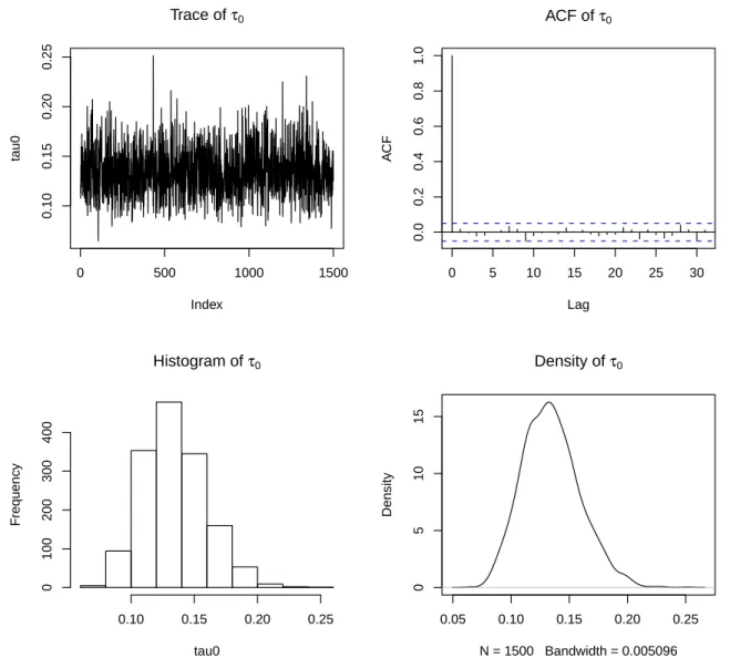
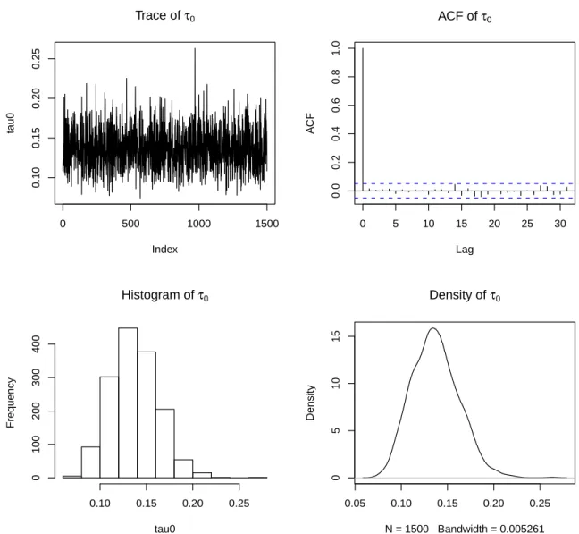
limit (red), estimated excess death rate (green) by month and influenza epidemic periods (grey rectangles) for the study causes of death - age group ≥ 85 . . . 112 C.1 Trace, autocorrelation function, histogram and density of τ0parameter
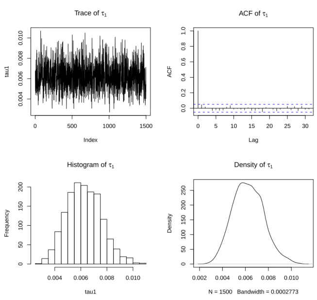
of model 0 . . . 116 C.2 Trace, autocorrelation function, histogram and density of τ1parameter
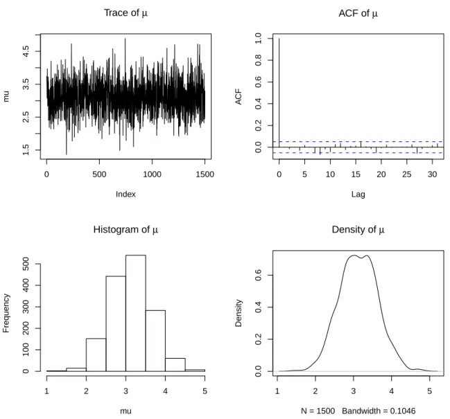
of model 0 . . . 117 C.3 Trace, autocorrelation function, histogram and density of µ parameter
of model 0 . . . 118 C.4 Trace, autocorrelation function, histogram and density of β1parameter
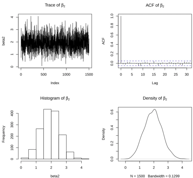
of model 0 . . . 119 C.5 Trace, autocorrelation function, histogram and density of β2parameter
of model 0 . . . 120 C.6 Trace, autocorrelation function, histogram and density of θ0parameter
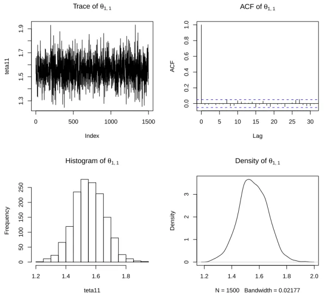
of model 0 . . . 121 C.7 Trace, autocorrelation function, histogram and density of θ1,1
param-eter of model 0 . . . 122 C.8 Trace, autocorrelation function, histogram and density of θ1,2
LIST OF FIGURES xxv
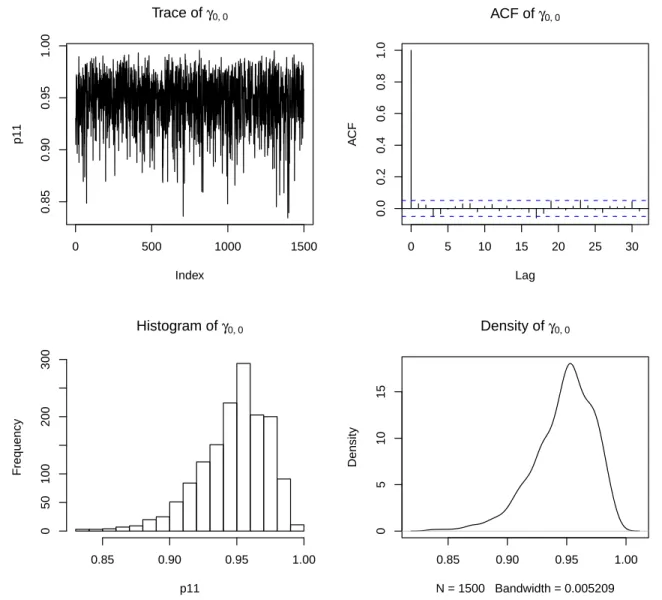
C.9 Trace, autocorrelation function, histogram and density of γ0,0
param-eter of model 0 . . . 124 C.10 Trace, autocorrelation function, histogram and density of γ0,1
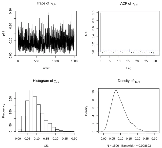
param-eter of model 0 . . . 125 C.11 Trace, autocorrelation function, histogram and density of γ1,0
param-eter of model 0 . . . 126 C.12 Trace, autocorrelation function, histogram and density of γ1,1
param-eter of model 0 . . . 127 C.13 Trace, autocorrelation function, histogram and density of τ0 parameter
of model 1 . . . 128 C.14 Trace, autocorrelation function, histogram and density of τ1 parameter
of model 1 . . . 129 C.15 Trace, autocorrelation function, histogram and density of µ parameter
of model 1 . . . 130 C.16 Trace, autocorrelation function, histogram and density of β1parameter
of model 1 . . . 131 C.17 Trace, autocorrelation function, histogram and density of β2parameter
of model 1 . . . 132 C.18 Trace, autocorrelation function, histogram and density of θ0 parameter
of model 1 . . . 133 C.19 Trace, autocorrelation function, histogram and density of θ1,1
param-eter of model 1 . . . 134 C.20 Trace, autocorrelation function, histogram and density of θ1,2
param-eter of model 1 . . . 135 C.21 Trace, autocorrelation function, histogram and density of α0,0
param-eter of model 1 . . . 136 C.22 Trace, autocorrelation function, histogram and density of α0,1
param-eter of model 1 . . . 137 C.23 Trace, autocorrelation function, histogram and density of α1,0
param-eter of model 1 . . . 138 C.24 Trace, autocorrelation function, histogram and density of α1,1
param-eter of model 1 . . . 139 C.25 Trace, autocorrelation function, histogram and density of τ0 parameter
C.26 Trace, autocorrelation function, histogram and density of τ1parameter
of model 2 . . . 141 C.27 Trace, autocorrelation function, histogram and density of µ parameter
of model 2 . . . 142 C.28 Trace, autocorrelation function, histogram and density of β1parameter
of model 2 . . . 143 C.29 Trace, autocorrelation function, histogram and density of β2parameter
of model 2 . . . 144 C.30 Trace, autocorrelation function, histogram and density of θ0parameter
of model 2 . . . 145 C.31 Trace, autocorrelation function, histogram and density of θ1,1
param-eter of model 2 . . . 146 C.32 Trace, autocorrelation function, histogram and density of θ1,2
param-eter of model 2 . . . 147 C.33 Trace, autocorrelation function, histogram and density of α0,0
param-eter of model 2 . . . 148 C.34 Trace, autocorrelation function, histogram and density of α0,1
param-eter of model 2 . . . 149 C.35 Trace, autocorrelation function, histogram and density of α0,2
param-eter of model 2 . . . 150 C.36 Trace, autocorrelation function, histogram and density of α1,0
param-eter of model 2 . . . 151 C.37 Trace, autocorrelation function, histogram and density of α1,1
param-eter of model 2 . . . 152 C.38 Trace, autocorrelation function, histogram and density of α1,2
List of Tables
2.1 Classification of the proposed methods for comparison, according to the fitting procedure (iterative or not), the model (seasonal ARIMA or cyclic regression) and the Ea periods (fixed period or a period
esti-mated by the national Influenza Surveillance Systems, ISS). T repre-sents the dimension of the training set. . . 16 2.2 Definition of the epidemic periods Eafor the flu-years 1980-81 to
2003-04 (NA: not available). Incidence values are presented by 105
inhabi-tants. From 1980-81 to 1989-90 epidemic periods were defined by the influenza death cause criterium, from 1990-91 to 2003-04 the epidemic periods were defined by the Influenza Surveillance System. . . 19 2.3 Correlation between the estimates of the influenza excess deaths,
ob-tained by different methods. . . 22 2.4 Output of flubase: excess deaths estimates for each Eaperiod,
consid-ering Ea periods as fixed and the non iterative procedure with cyclical
regression model. . . 25 2.5 Output of the flubase: excess deaths estimates for each Ea period,
Ea periods provided by the user and the non iterative procedure with
a seasonal ARIMA model. . . 26 2.6 Excess deaths estimates for each Ea period (including the 2003
heat-wave), Eaperiods provided by the user and the non iterative procedure
with a cyclical regression model. . . 28 xxvii
3.1 Characterization of influenza seasons from 1980-1981 to 2003-2004 ac-cording to the duration of the epidemic periods, dominant (sub)type of influenza virus, all causes influenza associated excess absolute deaths and age-standardized death rates. ISS: Influenza surveillance system, ISM: Influenza specific mortality. * Information is based on ILI surveil-lance and influenza virus activity; x - no epidemic period detected; NA, data not available.; Month numbers 1-January to 12-December ** In-formation on the season dominant type of virus for seasons 1982-83 to 1989-90 was obtained from the WHO. From 1990-91 to 2004-05 this information was obtained by the Portuguese ISS. . . 42 3.2 Average rates of excess mortality associated with influenza epidemics
and proportion of deaths attributable to influenza by disease outcome, age group, and dominant viral subtype, Portugal 1980-2004. Rates are per 100,000 population. * age-standardized rates; % IS: proportion of winter death attributable to influenza; calculated as the ratio of excess deaths to death occurring from October to May, by age group, mortality outcome, and season; ** Mann-Whitney test for comparison of excess mortality during A(H3) and A(H1) or B seasons; *** data not presented due to small death counts . . . 43 3.3 Correlation matrix between seasonal age-standardized excess rates.
In-juries are used as a control time series which should not be associ-ated with influenza virus circulation. CVD: cardiovascular disease; IHD: ischemic heart disease; DRS: diseases of the respiratory sys-tem: PI: Pneumonia and Influenza; CRD chronic respiratory disease: * p < 0.05; (1) correlation with ILI was only performed for the group of 65 and plus years of age. . . 45
4.1 Natural logarithm of the marginal likelihoods of the proposed models. 78 4.2 Posteriori means and 95% credible intervals for model parameters. NA:
not applicable. . . 78 4.3 Estimated influenza epidemic periods by proposed models for a
poste-rior probability of being in the epidemic state higher than 0.5. Values represent week/year. . . 81
LIST OF TABLES xxix
A.1 Seasonal ARIMA best-fitted models by R package forecast and Box-Ljong test for residuals auto correlation . . . 104 B.1 Sensitivity analysis: excess deaths and age-standardized excess death
rates from injuries that are ”attributable to influenza” by the used method. Injuries comprise all external causes of death. . . 114
Chapter 1
Introduction
Influenza is an acute respiratory infection that, in the temperate climates, during Autumn and Winter, is responsible for epidemics of considerable dimension, with attack rates that vary between 5 and 10% of the general population and with duration of 2 to 26 weeks [1, 2].
During these epidemic periods, influenza is associated with an increase of morbid-ity and mortalmorbid-ity from all causes, mainly in the individuals with 65 or more years of age. Nevertheless the burden of influenza can also be high in the younger age groups, usually during pandemics, like 1918-19, 1957, 1967 and 2009-10 [3, 4, 5].
In Europe it is acknowledged that seasonal influenza epidemics are responsible for an average of 40,000 deaths per season, an important increase in the need for health services capacities and also for a big impact in the labor force given the considerable absenteeism they originate [6]. Given the substantial impact of the influenza epi-demics in the human populations, public health surveillance systems were established since 1952, when the World Health Organization (WHO) launched the WHO Global Influenza Surveillance Network. This network is based on the National Influenza Cen-ters that collect and send biological samples from patients with influenza-like illness (ILI) to WHO Collaborative Centers for antigenic and genetic analysis. The main objective of this network is to recommend the content of the influenza vaccine and serve as a global alert mechanism for an influenza virus with pandemic potential [7]. Further more, to monitor the impact of influenza epidemics in the mortality and morbidity of the populations other systems were also implemented. Examples are: the 122 Cities Mortality Reporting System, managed by the United States Center
for Disease Control and Prevention (US CDC), that collects weekly the number of deaths due to Pneumonia and Influenza (P&I) by age group in 122 cities of the US [8]; the Euro-MOMO project that collects the weekly mortality from all causes in a network of 13 European countries [9]; the European Influenza Surveillance Network that is based on sentinel networks of general practitioners (GP) that report on a weekly basis the ILI incidence rate [6]. All these surveillance systems have the ob-jective of supplying to the health authorities information to perform up-to-date risk assessments for public health action, i.e. implement measures to control and miti-gate the epidemics impact. Generally, information provided by these systems helps the health authorities in following the influenza epidemic evolution, week by week, in terms of the epidemic onset, peak and end, and also in terms of its impact and severity, measured as excess of medical consultations, hospitalizations and mortality. For these purposes, several statistical methods have been proposed and applied to the data collected by these surveillance systems. The reason for the first studies was the 1918-19 influenza pandemic. To access the impact of this event, Collins SD (1957) [10] suggested an ecological method that estimates the monthly expected mortality rate in the absence of the influenza epidemic and subtracts the observed mortality rates from the expected. The sum of these excesses during the epidemic period was considered as the excess mortality attributable to the pandemic.
In fact, this rational of defining baselines that describe an indicator behavior in the absence of public health threats has been the basis for the majority of the statistical methods that were presented, from then to nowadays, to identify the start of a public health event and to estimate its impact.
Another important feature of the public surveillance system, operating for several years, is the richness of information it contains, which could allow short term fore-casting of indicators under analysis. For some situations, this short term forefore-casting is indeed a nowcasting, given that surveillance systems usually report information with a delay of one or more weeks, and a one or two weeks forecast is, in practice, a prediction of the current situation, i.e. a nowcasting. The application of statistical methods to predict the present situation or the near future, can greatly contribute to reduce the surveillance system timeliness and enhance the up-to-date epidemic risk assessment.
On this subject some works have also been presented with relative success [11, 12], nevertheless none has shown to be sufficiently practical to be implemented week by
3
week as a new outbreak indicator of the surveillance system. In this context, the main research objectives of this thesis are:
1. To unify in a single class the statistical methods characterized by using inter-rupted mortality time series to estimated excess deaths attributable to influenza epidemics, in order to describe and compare their applicability and results; 2. To estimate the excess mortality associated with the influenza epidemics
oc-curred in Portugal in the period from 1980 to 2004 and compare the results with those from other locations;
3. To develop a statistical model to nowcast the influenza epidemic evolution. In general, for the first objective, the research focused on the group of methods characterized by not considering influenza activity covariates to model the mortality baseline and by excluding from the model fitting process all the parts of the mortality time series where there was evidence of influenza epidemics occurrence. So, to describe this group a comprehensive review of the main proposed methods [13, 14, 15, 16, 17, 18, 19] was carried out with the aim of finding not only their unifying characteristics but also their differences. The identified features were then used to set a general framework that encompasses them all. Finally, to compare the methods and the impact of each feature on the estimates of the excess deaths associated with influenza epidemics, the different methods were applied to the time series of deaths by P&I in Portugal from 1980 to 2004 [20].
To accomplish the second goal the method that in [20] was shown to be more appropriate to retrospectively estimate the excess deaths attributable to influenza epidemics was elected to be applied to the Portuguese mortality data in the period of 1980 to 2004. So, given that the last study on the burden of influenza epidemics in Portugal [21] was focussed only on excesses of all causes and P&I deaths for all ages and for the elderly (≥ 65 years) in the period from 1990 to 1998, this new work [22] has analyzed the mortality time series for 7 causes of death (all causes, cerebrovascular disease, ischemic heart disease, diseases of the respiratory system, chronic respiratory diseases, and pneumonia and influenza) and 8 age groups (0-4, 5-54, 55-64, 65-69, 70-74, 75-79, 80-84 and ≥ 85).
Finally, to achieve the last research objective, to nowcast the influenza epidemics evolution, in a public health surveillance system setting, a statistical model, within
the family of the hidden Markov models (HMM), was developed. This class of models was chosen not only because some success in outbreak detection problems has already been accomplished with this framework [23, 24, 25], but also because it was further noticed that it can enable the nowcast of two important measures, simultaneous: the probability of being in the epidemic state and the ILI incidence rate. Within the HMM family the state transition probabilities can be assumed constant in time or time-variant, respectively corresponding to a homogenous or non homogenous HMM. For this work, the non homogenous model was the elected one, because it has the advantage of allowing the inclusion of time-variant covariates with early information on the epidemic evolution to model not only the response variable, the ILI weekly rate, but also the state transition probabilities from the non epidemic to the epidemic state and vice-versa. To our knowledge, this work [26] represents the first attempt to use non homogenous HMMs in a disease surveillance problem with the objective of early detect an outbreak and nowcast its evolution.
The thesis is organized as follows. Chapter 2 focuses on the methods used to estimate excess deaths attributable to influenza epidemics. Hence, after an introduc-tion to these methods (Secintroduc-tion 2.1) and the presentaintroduc-tion of some essential concepts (Section 2.2) a description of the most relevant methods is made in Section 2.3. A general framework proposed with the objective of finding a common ground between the methods, to describe and compare them, is then given in Section 2.4. The com-parison between the methods is exemplified by the application of all class methods to the time series of deaths due to P&I in Portugal from 1980 to 2004 (Section 2.5). In Section 2.6 a set of user friendly R-routines, package flubase [27], which implement all methods is briefly presented. The main results are then discussed in Section 2.7.
The estimates of excess mortality rates associated with influenza virus circulation in Portugal, during the period of 1980 to 2004, is presented in Chapter 3. An intro-duction to the impact of influenza epidemics in terms of excess mortality is given in Section 3.1. The data description is presented in Section 3.2 and the method used to estimate the epidemic periods and the excess deaths (selected from the framework presented in Chapter 2) are presented in Sections 3.3 and 3.4. Section 3.5 describes the main results and the specificity analysis applied to evaluate the method robust-ness. Finally, Section 3.6 frames the obtained estimates in the published literature and discusses the main differences and similarities between countries, geographical regions and population characteristics.
5
In Chapter 4 the development of a non homogenous HMM to nowcast the influenza activity in the context of a public health surveillance system is presented. Section 4.1 introduces the motivation, the question of timeliness of a public health surveillance system and the need to have predictions of the current situation. An overview of the HMMs and their application to the influenza surveillance problem is then given in Section 4.2, along with the formalization of the non homogenous HMM. At Section 4.3, the data used for the application example is introduced, the Portuguese influenza surveillance system (ISS) from week 40/2008 to week 16/2011. In Sections 4.4 and 4.5 the specific models proposed are described along with the bayesian approach for the model parameters estimation and for nowcasting the current ILI rate and influenza activity state. Section 4.6 details the results, both the application of the models to the entire data set as well as the real-time nowcast of the 2010-11 influenza season. In section 4.7 the model and results are discussed.
Finally Chapter 5 presents the main conclusions about the research objectives and suggestions for future developments.
Chapter 2
Time series methods for
obtaining excess mortality
attributable to influenza
epidemics
1
2.1
Introduction
In the Northern Hemisphere countries, during influenza epidemic periods, a rise in mortality from all causes is usually observed, mainly in the elderly population (aged 65 years or more) [28]. This increase can be associated with influenza epidemics since the influenza infection might cause complications that can lead to the hospitalization and/or death of the infected individual [36, 37]. In this context, and from a public health point of view, the quantification of the influenza epidemics impact on the pop-ulation and its description in terms of the dominant virus strain and level of vaccine coverage is of the utmost importance. The measurement of influenza impact in terms of deaths hospitalizations is never accessed by the number of deaths with influenza as the main cause in national mortality registries because this value is usually very low, even during the most severe epidemics. This is mainly due to the difficulty in estab-1This Chapter is based on the paper Nunes B, Nat´ario I, Carvalho ML. Time series methods
for obtaining excess mortality attributable to influenza epidemics. Statistical Methods in Medical Research. 2011; 20(4):331-346. Epub 2010 March 8.
lishing a connection between a complication (pneumonia or other respiratory diseases, circulatory system diseases, etc) and a previous or current influenza infection, due to the lack of a laboratory confirmed diagnosis. As a consequence, the use of official death registries, with influenza as cause to measure the influenza epidemic impact would underestimate its real effect [28]. This has led researchers to look for reliable methods to estimate influenza-associated deaths, using as a starting point a mortality time series and, when available, additional information from influenza epidemiologic surveillance systems on the seasonal epidemic characteristics. Generally, the methods used to estimate the excess deaths attributable to the influenza epidemics follow three steps:
1. Obtaining a baseline of the number of deaths, by a certain time unit, in the absence of influenza epidemics;
2. Using the baseline to identify the periods where there is evidence of an excess of deaths attributable to influenza epidemics;
3. Subtracting this baseline from the observed number of deaths, during these periods.
In this sense, the observed excess of deaths above the baseline, when associated with influenza epidemic periods, could, in the absence of other explainable events, be attributed to an influenza epidemic. The state-of-the-art of the methods to estimate the excess deaths attributable to influenza epidemics offers a large variety of different alternatives, all applicable to identical situations and aiming essentially the same purpose. These methods can be classified into two general methodological approaches and, within those, they vary in a considerable number of aspects.
In the first group, the methods are based on statistical models that include in-fluenza activity indicators as explanatory covariates. The pioneer ones [29, 30, 31] are multiple regression models including a polynomial function of time for trend, dummy variables for month effect to cope with seasonal variation, the monthly mean of weekly minimum temperature and the monthly ILI incidence rate as an influenza activity indicator. Later, [32, 33, 34] propose a Poisson regression model including, in general, the same type of variables, except [33] that uses one influenza activity indicator by each sub-type of influenza virus, A(H3), A(H1) and B, plus an indicator of the respi-ratory syncytial virus activity, all considered as proportion of isolates by week. Thus,
2.1. Introduction 9
this type of method enable the estimation of influenza burden by sub-type taking into account the possible simultaneous effects of other factors in mortality, like the effect of climate and/or other respiratory infections. These methods are very exigent in terms of external data needed and are also dependent on the accuracy of the in-fluenza activity indicators used that are, in general, based on sentinel surveillance systems, which are known to be sometimes influenced by external factors like holiday periods (e.g Christmas and New Years Eve) [35].
The methods in the second group are characterized by not considering covariates and also by excluding from the estimating process all the parts of the mortality time series where there is evidence of influenza epidemics occurrence. This Chapter will be focused on this second group of methods. A close analysis of this group shows several differences among them, essentially on the type of statistical model employed (cyclical regression [14, 15, 16, 17, 18] or Autoregressive Integrated Moving Average (ARIMA) models [13, 19]), on the method used to build the baseline (non iterative [17, 16, 18] or iterative [14, 15, 13, 19]) and on the choice of the periods to be excluded from the mortality time series (epidemic periods defined using ILI surveillance systems [14, 17, 13, 19] or fixed periods, like December to April [15, 16, 18]). All these differences can lead to unequal influenza-associated deaths estimates. Differences between reported estimates have been identified leading specialists into a profound discussion without a final agreed conclusion [38, 39].
Here we were able to unify these methods in a single class, in such a way that it allows the description and comparison of their applicability and results. This proved to be an important step in the conceptualization of the statistical methods used to estimate influenza-associated deaths, clarifying all the steps performed and options taken to compute the desired estimates. This unification was also the basis to build an R-package, the flubase, that easily estimates the influenza-associated deaths by any of the methods in the class. This platform is quite user friendly even for those less familiarized with the theoretical statistical developments that have led to the results. The application of this tool could also empower other researchers to critically analyze the differences and similarities between the estimates obtained with a variety of method choices, allowing in this way a more comprehensive analysis of their data.
2.2
Some essential concepts
2.2.1 Influenza epidemic period, influenza season and flu-year
An influenza epidemic is defined as the occurrence, in a specific population, of a number of cases of influenza above what is usually expected, during a certain period of time, referred as the epidemic period. Usually the epidemic periods are unknown and therefore must be estimated.
The annual fixed period of time during which the influenza epidemics might occur, starting sooner or later, with larger or smaller duration, is named influenza season. In Portugal as in other northern hemisphere countries, this period starts in October of each year ending in May of the next calendar year. This is the period when the ISS are more active, as the occurrence of an influenza epidemic outside this period has an almost null probability. Taking into account the beginning and ending of the influenza season, a flu-year a is defined as the 52 (or 53 when the first calendar year of the flu-year is bissextile) weeks that start at week 27 of any calendar year n and ends at week 26 of the calendar year n + 1.
Let Ea denote the estimate of an influenza epidemic period occurred during flu
year a (Figure 2.1). The choice of these periods is greatly dependent on the level of information one has on the occurrence of influenza cases and on the temporal evolution of the influenza incidence rate in the population. In fact, to obtain a correct diagnosis of influenza, a confirmation of the influenza virus presence is necessary, procedure that is not usually carried out. In the majority of the situations only the clinical diagnosis are obtained, without the laboratory confirmation, and if this situation occurs the case can only be classified as ILI.
Therefore, the information that is usually available consists on the temporal evo-lution of the ILI incidence rates, complemented by information on the influenza virus circulation among the population. In the majority of the developed countries this information is collected by surveillance systems specifically designed for the effect, that are based on a sample of individuals set under surveillance.
When this information does not exist, or it is not available, some authors [16, 18] have set Ea as the fixed time period, enclosed in the influenza season period, that
goes from December to April of the next calendar year. Other solution is to use the time series of mortality specific by influenza (ICD 9th Revision:487; ICD 10th Revision:J9-J11) and define Ea as the periods where the mortality by influenza rises
2.2. Some essential concepts 11
above the expected. In principle, given the under registration of deaths with influenza as a cause, this last option should be a less sensible but more specific method, for the reasons we have mentioned earlier.
Week
Number of deaths P&I
27 36 45 1 7 15 24 33 42 51 6 14 23 32 41 50 6 14 23 0 25 50 75 100 150 200 250 300
Weekly number of deaths Mortality baseline
Mortality baseline upper threshold
Ea Ea
Da Da
yt, a
βt, a
Figure 2.1: Exemplification of the basic concepts.
2.2.2 Time series of the weekly number of deaths
Consider yt,a to be the time series of the number of deaths observed in week t,
t = 1(27), ..., 52(26)2 of year a, a = 1, ..., A, where A represents the number of flu-years in study. This time series is the main object of analysis, since the major goal is to estimate from it the excess number of deaths attributable to influenza epidemics. Usually the most used time series is the weekly (or monthly) number (or rate) of deaths by all causes or P&I.
2.2.3 Periods with excess deaths attributable to influenza epidemic
Define Daas the period of weeks where an excess of deaths in yt,a is attributed to
an influenza epidemic, in flu-year a. This period, included in the Eaperiod, is defined
by an observed increase in yt,a, above the expected in the absence of the effect of an
influenza epidemics (Figure 2.1). Additionally, during this period, there must be no other events that can be the cause of the observed excess deaths.
2.2.4 Mortality baseline in the absence of the influenza epidemics effect
Excluding from the time series the parts where there is some evidence of an influenza epidemic occurrence, one obtain the following interrupted time series, denoted here-after by y?
t,a = {yt,a: (t, a) /∈ Ea}.
Let βt,a be the baseline (Figure 2.1) resulting from fitting a statistical model to
the time series yt,a? or, as some authors have considered, to xt,a, the weekly number
of deaths in the absence of the influenza epidemics, defined as follows:
xt,a = ( yt,a, (t, a) 6∈ Da; ˜ yt,a, (t, a) ∈ Da (2.1)
where ˜yt,a represents some preliminary estimate of the weekly number of deaths in
the absence of the effect of an influenza epidemics for the week t of the flu-year a.
2.3
Description of methods in study
The studied methods are all characterized by obtaining a mortality baseline in the absence of influenza epidemics effects using an interrupted mortality time series. Gen-erally these methods fit a statistical model to y?t,ato obtain a baseline βt,athat is used
to identify the periods with excess deaths attributable to an influenza epidemic, Da.
To be able to jointly describe all these procedures one has to identify the unifying characteristics and also their differences in order to summarize them in a few classes. Three sources of dissimilarity were found.
1. Statistical model used to fit the interrupted time series: There are mainly two types of models used in the literature:
2.3. Description of methods in study 13
(a) multiple linear regression models [14, 15, 16, 17, 18], using a polynomial component to explain the series trend and a sinusoidal component that captures the seasonality observed - cyclical regression. Generally these models are given by:
ys= α + m X i=1 aisi+ l X j=1 b1,jsin j2πs 52 + b2,jcos j2πs 52 + εs
where ai, i = 1, ..., m, are the parameters of the order m polynomial
function used to explain the trend, b1,j and b2,j are the parameters of
the sinusoidal function with periods 52/j, j = 1, ..., l, used to explain the eventual seasonality and εs∼ N (0, σ2) with s = t + (a − 1)52, t = 1, ..., 52
and a = 1, ..., A.
(b) seasonal ARIMA[40] only applied in [13, 19] to this problem.
2. Choice of the Ea periods: In some of the reviewed papers this period was
the epidemic period defined (estimated) by the operating ISS, using data on clinical diagnosis of ILI and viral strains isolates [14, 17, 13]. In this case the a priori chosen Ea periods are different from flu-year to flu-year.
Other authors [15, 16, 18] defined Eaas a fixed set of weeks (December to April),
in each flu-year, where the occurrence of an influenza epidemic with effects on mortality is more likely. This period is always included in the influenza season. 3. Procedure used to fit the statistical model and to identify the Da
periods
(a) Non iterative (Figure 2.2): the model is fitted to all points of the inter-rupted time series y?
t,a [16, 17, 18] at once. Here the baseline βt,a
corre-sponds to the estimated values given by the model for each week t. In [17] the Daperiods are defined as the set of weeks, contained in the Eaperiods,
that initiate with two consecutive weeks with a number of deaths above the upper 95% confidence limit of the baseline and end with two consecutive weeks with a number of deaths bellow the same upper limit. Note that [16, 18] have defined the Daperiods applying the previous method only to
Week
Number of deaths P&I
27 44 7 22 39 1 16 33 50 15 32 49 14 31 48 13 30 47 12 0 25 50 75 100 125 150 175
200 Weekly number of deaths
Mortality baseline Mortality baseline threshold Excess mortality
Figure 2.2: Non iterative procedure used to fit the statistical model and to identify the Da periods. Grey boxes represent the Ea periods and yellow boxes represent the
Da.
(b) Iterative (Figure 2.3): generally, these methods consist in forecasting a baseline for each flu-year i using a statistical model fitted to xt,a for a
training set of T previous flu-years. This training set can have a fixed dimension T (equal for all iterations, e.g. 5 years) [14, 15], or be given by all previous years of flu-year i of that iteration [13]. In the iterative methods, Di is identified in each iteration i as the period of weeks contained in the
correspondent Ei period that initiates with two consecutive weeks with a
number of deaths above the upper 95% confidence limit of the forecasted baseline and terminate with two consecutive weeks with number of deaths bellow the same upper limit. After the Di identification the series xt,a is
2.4. General framework 15
by the values of the forecasted baseline, obtaining a preliminary estimate of the mortality time series in the absence of influenza epidemic ˜yt,aduring
those periods. Other authors simply use an interrupted time series where the values in the Di periods are excluded from the original time series.
Week
Number of deaths P&I
27 44 7 22 39 1 16 33 50 15 32 49 14 31 48 13 30 47 12 0 25 50 75 100 125 150 175 200
Number of flu−years used to forecast the next flu−year Weekly number of deaths
Mortality baseline fitted Mortality baseline forecasted Mortality baseline fitted forecasted Excess mortality
Figure 2.3: Iterative procedure used to fit the statistical model and to identify the Da period. Grey boxes represent the Ea periods and yellow boxes represent the Da.
2.4
General framework
Given the above description it is possible to accommodate a large number of meth-ods in a wide framework of methmeth-ods varying according to the three points considered, model fitting procedure, type of model and period where to identify the excess mor-tality periods attributable to the influenza epidemics Da - see Table 2.1.
Name Alias Model Period Fitting procedure T
It_RM_F [15] Regression Fixed period Iterative 5
It_RM_E [14] Regression ISS Iterative 5
It_SA_F none SARIMA Fixed period Iterative all previous years
It_SA_E [13] SARIMA ISS Iterative all previous years
RM_F [18, 16] Regression Fixed period Non iterative NA
RM_E [17] Regression ISS Non iterative NA
SA_F none SARIMA Fixed period Non iterative NA
SA_E none SARIMA ISS Non iterative NA
Table 2.1: Classification of the proposed methods for comparison, according to the fitting procedure (iterative or not), the model (seasonal ARIMA or cyclic regression) and the Ea periods (fixed period or a period estimated by the national Influenza
Surveillance Systems, ISS). T represents the dimension of the training set.
Note that it was possible to further identify three new methods, never considered before, from taking all possible combinations of alternatives:
1. It_SA_F iterative, using the the seasonal ARIMA model with Eaperiods fixed;
2. SA_F and SA_E that apply the seasonal ARIMA models with a non iterative procedure.
The It_SA_F does not seem to present any practical application problems. For methods SA_F and SA_E we propose to adjust a cyclic regression model to the inter-rupted time series, substitute then the Ea periods by the model expectations, and
then apply the seasonal ARIMA models to this new series.
In order to be able to compare all the methods described in Table 2.1 we had to address the following difficulties:
1. Evaluation of the adjustment quality of the baseline βt,a to the original time
series yt,a for (t, a) /∈ Da. Given that the objective is to estimate a baseline free
of excess mortality, the model is not fitted to the observed data during these Da periods. This condition makes unfeasible the direct application of the more
used goodness of fit measures (AIC, BIC, etc.), since the Da periods and the
resulting baseline differ from method to method. To overcome this we have considered the following measures for the baseline outside the Da:
2.5. Application example 17
• Residual Mean Square
RM S = X (t,a) /∈Da ˆ e2 t,a m
where m is the number of weeks without excess deaths attributable to influenza ˆet,a= yt,a− βt,a for (t, a) /∈ Da;
• Autocorrelation function of the residuals;
2. The true number of excess deaths attributable to influenza epidemics for each flu-year a is unknown. Therefore, the evaluation of the methods considering their excess deaths estimates was accomplished by:
• comparing, in each flu-year a, the estimated excess deaths attributable to influenza epidemics given by each method, and identifying those that estimate the higher and lower values of excess deaths;
• calculating the correlation between the estimates of the influenza excess deaths, obtained by different methods, as an empirical concordance mea-sure.
2.5
Application example
The analyzed data consists on the weekly number of deaths by P&I in Portugal from 1980-81 to 2003-04 flu-years obtained from the National Mortality database of the Portuguese Statistics Institute (Figure 2.4).
As presented in Table 2.2 the Ea periods were either set as fixed periods (from
week 48 (December) to week 17 (April)) or equal to the non fixed epidemic periods that were defined as follows:
• From 1980-81 to 1989-90 the influenza epidemic periods were defined using the weekly number of deaths by influenza (ICD 9th Revision 487). These periods were set as the consecutive weeks (more than two) with the number of deaths above the 95 percentile of the empirical distribution of the weekly number of deaths by influenza in the period comprised by the flu-years 1980-81 to 1989-90; • For the flu-years from 1990-91 to 2003-04 the epidemic periods used were the ones defined by the Portuguese ISS, of the Instituto Nacional de Sa´ude
Weekly deaths by Influenza and Pneumonia Time n umb er of deaths 1980 1985 1990 1995 2000 2005 50 100 150 2 00 2 50
Figure 2.4: Distribution of the weekly number of deaths by influenza and pneumonia in Portugal from 1980-81 to 2003-04.
Dr.Ricardo Jorge (of National Health Institute Dr. Ricardo Jorge) [41]. The final classification is presented in Table 2.2.
In this time series we have also substituted the known heat-waves periods [42] by the average of the number of deaths in the last week before and the first week after the heat-wave.
The models used in the application example were chosen in the following way: 1. The cyclic models used were chosen by a regular best fit model criteria, in a
preliminar analysis.
• non iterative procedure:
ys= α + β1s + β2s2+ β3s3+ b1sin
2πs
52 + b2cos 2πs
2.5. Application example 19
Epidemic periods (weeks) flu-year start peak end no
weeks max incidence
1980-81 49 3 12 16 NA 1981-82 - - - - NA 1982-83 1 2 7 7 NA 1983-84 10 11 12 3 NA 1984-85 3 3 4 2 NA 1985-86 52 3 3 4 NA 1986-87 - - - - NA 1987-88 - - - - NA 1988-89 - - - - NA 1989-90 1 3 6 6 NA 1990-91 7 9 11 5 148.4 1991-92 45 52 5 13 92.4 1992-93 6 11 14 9 117.7 1993-94 46 49 1 8 168.8 1994-95 3 5 8 6 84.1 1995-96 42 44 51 10 86.8 1996-97 47 50 8 15 111.3 1997-98 - - - - -1998-99 51 3 8 10 252.9 1999-00 2 5 8 7 156.5 2000-01 - - - - -2001-02 1 5 10 10 239 2002-03 48 50 50 3 76.1 2003-04 44 47 52 9 166.7
Table 2.2: Definition of the epidemic periods Ea for the flu-years 1980-81 to 2003-04
(NA: not available). Incidence values are presented by 105 inhabitants. From 1980-81 to 1989-90 epidemic periods were defined by the influenza death cause criterium, from 1990-91 to 2003-04 the epidemic periods were defined by the Influenza Surveillance System. • iterative procedure: ys= α + β1s + β2s2+ b1sin 2πs 52 + b2cos 2πs 52 + εs 2. The seasonal ARIMA models used were:
• non iterative procedure: chosen by an automatic model identification al-gorithm [43];
• iterative procedure: a model analogous to the one proposed in [13], ARIM A(2, 0, 0)(1, 1, 0)52:
(1 − φ1B − φ1B2)(1 − Φ1B52)∇52ys= εs,
In the present application example the Da periods were always defined as the set
of weeks, contained in the Ea periods, that initiate with two weeks with a number
of deaths by P&I above the upper 95% confidence limit of the baseline and end with two weeks with a number of deaths bellow the same upper limit.
2.5.1 Results
The methods that considered the Ea periods as fixed presented lower RMS than the
methods using year-variable size periods, estimated by the ISS. Within each of these two different groups (fixed period or ISS periods) it was observed that the seasonal ARIMA model always presented lower values of RMS when compared to the cyclic regression model – Figure 2.5. Autocorrelation in the residuals outside of the Da
periods was observed for all the methods that used cyclic regression models.
RM_F SA_F It_RM_F It_SA_F RM_E SA_E It_RM_E It_SA_E
0 50 100 150 200 R M S Methods
Figure 2.5: Residual Mean Square Errors of the studied models.
From Figures 2.6 and 2.7 it can be observed that when the Eaperiod is set fixed,
the number of influenza-associated estimated deaths is clearly higher. On the other hand, when the Ea periods are set by the ISS it is patent an higher uniformity in
the number of influenza-associated estimated deaths, between the methods. This observation was confirmed by the high correlation coefficients obtained between all methods for those using Eadefined by the ISS, that as can be seen in Table 2.3 are all
2.5. Application example 21
a greater disagreement between estimates after flu year 1993-1994 mainly when the Eaperiod was fixed.
Flu Year Influenza−associated deaths It_RM_F It_SA_F RM_F SA_F 80/81 83/84 86/87 89/90 92/93 95/96 98/99 01/02 0 200 400 600 800 1000 1400 1800
Figure 2.6: Estimated influenza-associated deaths from 1980-81 to 2003-2004 accord-ing to the type of method, consideraccord-ing Ea as a fixed period from week 48 (December)
RM_F SA_F It_RM_F It_SA_F RM_E SA_E It_RM_E It_SA_E RM_F 1 0.996 0.935 0.909 0.952 0.938 0.914 0.909 SA_F - 1 0.933 0.914 0.961 0.946 0.917 0.915 It_RM_F - - 1 0.793 0.924 0.926 0.932 0.915 It_SA_F - - - 1 0.885 0.872 0.831 0.854 RM_E - - - - 1 0.996 0.975 0.979 SA_E - - - 1 0.984 0.986 It_RM_E - - - 1 0.976 I_SA_E - - - 1
Table 2.3: Correlation between the estimates of the influenza excess deaths, obtained by different methods. Flu Year Influenza−associated deaths It_RM_E It_SA_E RM_E SA_E 80/81 83/84 86/87 89/90 92/93 95/96 98/99 01/02 0 200 400 600 800 1000 1400 1800
Figure 2.7: Estimated influenza-associated deaths from 1980-81 to 2003-2004 accord-ing to the type of method, consideraccord-ing Ea as defined by the Influenza Surveillance