Equity valuation : valuing Semapa as the sum of the parts

(1)

Equity Valuation

Valuing Semapa as the Sum of the Parts

Candidate:

Rute Carina Relho Cardoso

[email protected]

Supervisor:

Dr. José Carlos Tudela Martins

Dissertation submitted in partial fulfilment of requirements for the degree of MSc in

Business Administration, at the Universidade Católica Portuguesa

(2)

Equity Valuation – Semapa 2012

1 fnkjc

EQUITY RESEARCH

Semapa: An Active Equity Player

Semapa is a holding company currently owning (1) 75,85% of the pulp and paper producer Portucel, representing more than 90% of Semapa’s 2011 net profit (excluding holding costs); (2) 100% of the cement company Secil, which accounted for 8% of its 2011 net profit (excluding holding costs) when it just owned 51%; and (3) 96% of a small business related with the environment, ETSA, which contributed to less than 2% to Semapa’s 2011 net profit (excluding holding costs).

Semapa completed its most recent acquisition on May, 2012, when it bought the remaining 49% of Secil.

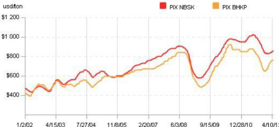
Portucel – still rocks. UWF paper and BEKP prices are currently 1%

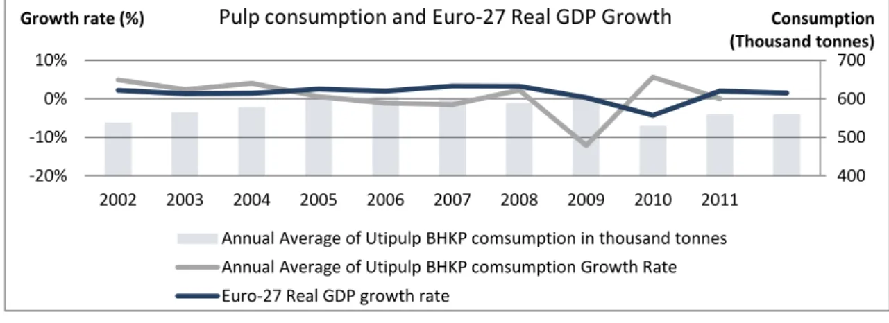
and 9% higher, respectively, than the last year’s average. The expected demand drop should be offset by the last year’s shutdowns in the industry, supporting higher paper volumes, although intensive competition from Asia is expected. With the new paper machine implemented in 2009, Portucel considerably reduced its exposure to the pulp prices, which presented a volatility of 116% during the past 11 years. With the capacity shutdowns in the industry and the need for more pulp to be integrated in the paper production, Portucel expects to be operating at near 100% of its total capacity. The strong USD may help Portucel to trigger exports. Moreover, the expected high consumption levels in the emerging markets may be a buffer of the prices’ volatility since those markets might absorb the excess supply verified in the developed markets.

Secil – the last acquisition. Semapa acquired the remaining 49% of

Secil on May, 2012, currently owning 100%. The construction sector has not been living its most prosperous days, but Secil has been able to sustain its performance by maintaining its market share in the principal markets and its geographical diversification is the best means of stabilizing its earnings. However, Secil still faces some risks on the countries it operates, such as Tunisia where the government has control over prices and exportations. Secil’s presence in Angola is being threatened by the Chinese producers who forced Secil to decrease its operating margins. Significant fluctuations on electricity and fuel costs can have a negative impact on the Secil’s business.

Pulp&Paper/Holding

BUY/BUY

September 2012

Portugal

Semapa Price as at 02-Jul-2012 (€): 52 Week range (€): No. Shares (mn): Market Cap (€mn): Price Target (€): 4,99 4,7-7,6 118,3 590,5 10,25

Source: Bloomberg and own calculations.

Source: Bloomberg. 0 2 4 6 8 10 A ug -10 Nov -10 Fe b -11 M ay -11 A ug -11 Nov -11 Fe b -12 M ay -12 Portucel Semapa PSI-20

Portucel/Semapa

Portucel Price as at 02-Jul-2012 (€): 52 Week range (€): No. Shares (mn): Market Cap (€mn): Price Target (€): 1,93 1,7-2,3 767,5 1.478 2,94

(3)

2

Portucel owns the largest and most efficient plants in Europe, all settled in

Portugal. It benefits from the vertically integrated production model (forest, pulp and paper) and from a strong portfolio of brands. Its clients are spread over 115 countries, with the markets excluding Europe and America growing considerably.

Different perspectives – Since the investment made in a new paper

machine in 2009, the paper UWF has been gaining weight on Portucel’s total revenues, which represented 79% last year. In one side, Portucel took advantage from the lower exposure to the volatile BEKP pulp prices, which are expected to vary 33% in the following years. But on the other side, BEKP prices registered an increment of 9,3% in relation to the previous year’s average while the UWF paper prices remained almost unaffected. All in all, the company was able to increase its cash flow generation and the recent capacity shutdowns in the industry are expected to hold Portucel’s capacity utilization rates at near 100%.

The third party – Starting by being self-sufficient, the renewable energy

currently represents around 11% of Portucel’s total revenues. However, the energy segment is expected to remain constant on Portucel’s portfolio, with the capacity utilization rate at no more than 90%.

Source: Portucel’s Annual Reports.

Source: Portucel’s Annual Reports, FOEX and own calculations.

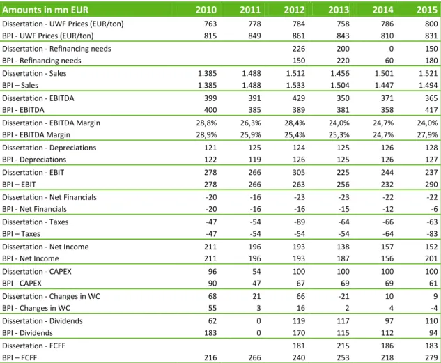
Portucel (mn €) 2010 2011 2012E 2013E 2014E 2015E 2016E 2017E

UWF Prices (EUR/ton) 763 778 784 758 786 800 783 779 BEKP Prices (EUR/ton) 540 492 551 451 445 415 445 471

Refinancing needs 226 200 0 150 150 150 Sales 1.385 1.488 1.512 1.456 1.501 1.521 1.508 1.529 EBITDA 399 391 429 350 371 365 325 318 EBITDA Margin 29% 26% 28% 24% 25% 24% 22% 21% Depreciations 121 125 124 125 126 128 129 130 EBIT 278 266 305 225 244 237 196 187 Net Financials -20 -16 -23 -23 -22 -22 -29 -33 Taxes -47 -54 -89 -64 -66 -63 -49 -46 Net Income 211 196 193 138 157 152 118 109 CAPEX 96 54 100 100 100 100 100 100 Changes in WC 68 21 66 -21 10 9 -10 0 Dividends 62 0 119 117 97 110 121 94 FCFF 181 215 186 183 177 163

Source: Portucel’s Annual Reports, FOEX and own calculations.

DCF Assumptions k Re 8,5% Beta 0,82 Rf 2% MRP 8,4% Rd 5,3% Ku 7,32% Banktuptcy Cost 30% Default Prob. 19,5% D/E 56% D/V 36% E/V 64% T 29,5% TGR 1,5%

Source: Bloomberg and own calculations.

Both Portucel’s EV/EBITDA and P/E multiples are expected to be higher in this year than they were in the previous one, which mirrors Portucel’s ability to overcome the global economic crisis. Despite Portucel’s good performance, its multiples are below the peer’s harmonic average.

EV/EBITDA P/E P/BV T12M 2012E 2011 2012E 2011 PORTUCEL 4,96 5,02 7,52 7,73 0,97 IP 6,65 5,53 10,81 8,32 1,79 SAPPI 5,56 3,94 10,65 7,68 1,06 HOLMEN 3,29 6,67 13,42 12,54 0,81 EMPRESAS CMPC 10,73 9,85 17,44 16,13 1,11 STORA ENSO 6,71 5,46 10,16 8,67 0,65 SHANDONG 6,13 9,35 8,55 1,52 Harmonic Average 5,71 5,81 11,46 9,61 1,03

9% 79% 11% Pulp BEKP Paper UWF Energy and Others 0 200 400 600 800 1000

Average Price BEKP - EUR/ton Average Price A4-Copy B - EUR/ton 2011’s Revenue Breakdown (€1488mn)

Expected Pulp and Paper Average Prices

(4)

3

Secil’s turnover is dependent on the level of activity in the building sector

in each of the geographic markets where it operates – Portugal, Tunisia, Angola, Lebanon and Cape Verde. The construction sector depends on the level of residential and commercial building, as well as on the level of investments in infrastructures. This sector is highly sensitive to macroeconomic factors, where a downturn in the economic activity may lead to a recession in the building industry.

The crisis’ damages – The Portuguese cement consumption is expected to

continue to decline in the near future. The excess capacity forced cement producers to decrease their prices and operate in an extremely competitive market. The reutilisation of residuals as energy and raw materials are part of Secil’s major concerns. The Angolan government imposed a policy of containment of public spending. Aligning this fact with a cement’s consumption decline and competition from Chinese imports, Secil’s performance in Angola is expected to slow down.

The importance of stability – The Lebanese government has been

demanding public works, contributing to an increment of 4% on Secil’s sales in 2011 and it is expected to keep increasing. The investment in a new cement mill in Tunisia will allow Secil to register maximum volume sales in the near future.

Source: Secil’s Annual Reports.

Secil (mn €) 2010 2011 2012E 2013E 2014E 2015E 2016E 2017E

Sales 535,8 506,9 488,1 493,7 510,0 527,7 548,1 571,3 Portugal 328,1 302,1 269,8 260,4 261,0 263,2 266,7 271,6 Tunisia 69,3 61,1 64,0 67,0 70,2 73,6 77,1 80,7 Lebanon 77,2 80,8 86,2 92,1 98,3 104,5 111,1 118,1 Angola 27,8 30,4 35,3 40,3 45,4 50,3 55,7 61,7 Others 33,5 32,5 32,8 33,9 35,0 36,2 37,5 39,1 EBITDA 114,9 65,2 91,6 88,5 86,2 83,6 80,8 77,9 EBITDA Margin 21% 13% 19% 18% 17% 16% 15% 14% Depreciations 81,9 85,1 63,3 63,9 65,5 67,0 68,6 70,2 EBIT 77,9 47,2 96,3 92,6 88,7 84,5 80,1 75,7 Net Financials -4,9 -6,2 -7,6 -6,6 -5,4 -6,1 -7,1 -8,7 Taxes -16,6 -10,2 -22,1 -21,4 -20,8 -19,5 -18,2 -16,7 Net Income 56,5 30,8 66,5 64,5 62,5 58,9 54,8 50,3 CAPEX 44,2 62,2 52,8 52,8 52,8 52,8 52,8 52,8 Changes in WC 4,0 -16,4 -9,1 0,6 1,5 2,2 3,0 3,5 Dividends 37,0 28,8 11,5 30,0 31,8 34,1 35,4 37,0 FCFF 93,7 81,6 79,1 77,0 74,7 72,8

Source: Secil’s Annual Reports and own calculations.

DCF Assumptions k Re 11,4% Beta 0,94 Rf 2% MRP 10,6% Rd 6,3% Ku 10% Banktuptcy Cost 30% Default Prob. 19,5% D/E 39% D/V 28% E/V 72% T 24,9% TGR 1,0%

The forecasted EV/EBITDA and P/E multiples are expected to be lower than Secil’s peer group harmonic average in the previous year. This is a reflection of the economic crisis that has been acting globally and affecting the construction sector the most. Secil’s relatively good performance is driven by its cost cut policy and diversified operations.

EV/EBITDA P/E

SECIL T12M 2012E 2011 2012E

CIMPOR 6,35 5,30 11,07 7,89 HOLCIM 8,07 6,68 61,40 12,07 HEIDELBERGCEMENT 6,52 5,96 19,23 9,58 SA DES CIMENTS 6,59 5,52 10,32 7,88 DYCKERHOFF 2,24 2,83 23,76 13,81 CIMENTS FRANCAIS 5,14 4,74 16,30 10,06 LAFARGE 10,56 9,02 18,92 15,66 Harmonic Average 5,30 5,14 17,00 10,35

60% 12% 6% 16% 6% Portugal Tunisia Angola Lebanon Others 0 5.000 10.000 2004 2005 2006 2007 2008 2009 2010

Cape Verde Lebanon Angola Tunisia Portugal

2011’s Revenue Breakdown (€507mn)

Cement Market Demand (‘000 tons)

(5)

4

Semapa No. Shares 02-07-2012 Equity DCF (mn €)

Portucel 75,85% 745,4 1,93 € MV 2.188,3

Secil 100% 515,6 mn € MV 638,5

ETSA 96% BV 25,8

- Semapa's Holding Debt 1.082,2

+ Semapa's Holding Cash 392,9

- Semapa's Holding Unfunded Pensions 100,1

- Semapa's Holding Cash Flows 377,7

Semapa 112,9 4,99 € MV 1.157,0

Semapa's Target Price (€): 10,25 Recommendation: Buy

Source: Companies’ Annual Reports and own calculations.

DCF Assumptions k Re 8,5% Beta 0,73 Rf 2% MRP 6,0% Rd 6,9% D/E 183% D/V 65% E/V 35% T 25,9% WACC 6,3% TGR 1,4%

(6)

i

Abstract

This dissertation aims to value the holding Semapa as the sum of the parts of the companies it owns – Portucel, Secil and ETSA. There is still much debate on which model is the best to estimate a company’s value, therefore the main methods and theories are firstly discussed in order to use the most appropriate valuation framework and accurate assumptions. By attributing different capital structures’ scenarios, this dissertation illustrates two Discounted Cash Flow’s approaches, as well as the value dispersion among them: the Adjusted Present Value with and without a target capital structure and the Weighted Average Cost of Capital. In comparison with the current market prices, the three models indicate that Semapa is currently undervalued. The multiples valuation are also performed as a complementary tool. The results obtained are then compared with those of BPI Equity Research and Millennium Investment Banking’s reports published in 2012 with the objective of doing a critical assessment on the main sources of differentiation.

(7)

ii

Acknowledgements

This dissertation represents a hard working process where I was challenged to apply my knowledgment in Equity Valuation and incur in deep research in order to take final decisions. Fortunately, I was able to rely on people who took important roles thoughout the whole process and to whom I would like to express my gratitude: Professor José Tudela Martins, with whom I discussed the main problems encountered, for his promptitude in replying my e-mails and for the valuable feedback; to Dr. Rui Menezes, Semapa’s Investor Relations Department, for the data provided and his kindness in answering my calls; to my colleagues for the constructive discussions, support and helpful feedback; and finally, to all my family and friends who have always stood by my side.

(8)

iii

1. Introduction

1.1. Dissertation’s Purpose

The present dissertation has the purpose of valuing a listed company. In order to accomplish this goal it will be necessary to discuss the most relevant articles where the lack of consensus rely the most and propose the most suitable models according to the company features. Then, after having reached a consensus, the chosen valuation approaches will be implemented in order to reach a target value and compare it to the current value. In the end, there will be a comparison between the valuation made in this dissertation and an Investment Bank’s report valuation, where the main differences are identified.

1.2. The Company

The company chosen is Semapa – Sociedade de Investimento e Gestão, SGPS, S.A. (hereon referred as “Semapa”) listed on the PSI-20 Stock Exchange. It currently owns 75,85% of Portucel – Empresa Produtora de Pasta e Papel, S.A. (hereon referred as “Portucel”), 100% of Secil – Companhia Geral de Cal e Cimento, S.A. (hereon referred as “Secil”) and 96% of ETSA – Investimentos, SGPS, S.A. (hereon referred as “ETSA”).

Portucel is a listed company, also on the PSI-20 Index, and its core business is on the pulp and paper production. Lately, Portucel has been investing heavily on the energy sector and its presence on the renewable energy already represents more than 5% of the total energy produced in Portugal. Since it is a price taker in what regards the pulp and paper products, Portucel has the particularity of being a cyclical company. Although Portucel exports more than 90% of its total revenues, all its subsidiaries are settled in Portugal.

On the other side, Secil is a producer of cement, concrete and aggregates. Besides Portugal, Secil also operates in Tunisia, Lebanon, Angola and Cape Verde. More than 50% of its total volume comes from exportation. The cement industry highly depends on the construction sector, which since 2002 has been suffering from the global crisis and the negative trend is expective to continue in the near future.

The two referred companies – Portucel and Secil – will be valued separately and, at the end, multiplied by the percentage owned by Semapa. Regarding ETSA, since it only contributes with less than 2% to the total revenues of Semapa, ETSA will be accounted for its book value.

(12)

2

1.3. Dissertation’s Structure

In order to cover the mentioned purpose, the dissertation will be the following:

a. In section 2, the literature review attempts to gather the main valuation concepts and methodologies in order to choose the approaches that best fits Portucel and Secil‘s features. It first starts by describing the main Discounted Cash Flow methods and then it goes into detailed considerations where relies a lot of controversy, such as tax shield, terminal value, equity risk premium and other discount factors. It is also described other valuation methodologies such as options, multiples and liquidation and accounting. For being in the presence of a cyclical company, it is also important to analyse what are the main considerations when value such companies.

b. Section 3 is responsible for the application of the methodologies described on the literature review. But before starting, it is important to perceive the industries where both Portucel and Secil are inserted in, so as the macroeconomic factors influencing their operational activity. Then, an overview of each company’s value drivers is undertaken by breaking down the historical data. This analysis is of extreme importance as the forecasted periods will contain some influence from past behaviours. When assumptions are required, it is of main priority to find and justify them as rational as possible;

After cover each company’s forecasted periods, the valuations of Portucel, Secil and Semapa are performed, as well as the respective price target and recommendation. The chosen method will be the Adjusted Present Value. Although there are several theories on that method, it will be chosen and justified a specific approach and further compared with other APV’s approach and the widely used WACC. It is also performed a sensitivity analysis in order to verify the consistency of this dissertation’s valuation. To conclude, the DCF valuation will be complemented with the multiples valuation; c. In section 4, this dissertation’s results, methodologies and assumptions are compared

with those of the selected research reports. The purpose is to perceive and justify which one followed the best approaches.

d. Section 5 will refer this dissertation’s final remarks and possible limitations encountered.

(13)

3

2. Literature Review

2.1. Introduction

There are several models and theories attempting to explain how to best value a company, but there is no right or wrong model, neither consensus regarding the best approach. Equity researchers are constantly working on the new market trends in order to provide analysts with the most suitable and precise models. However, the analysis will always depend on each one’s perspective.

The purpose of this chapter is to make reference to the most relevant theories and, according to the demonstrations, sample and conclusive arguments, to choose the models that better reflects the characteristics of the company under valuation.

2.2. Valuation Frameworks

Every analyst aspires to reach the true value. Although, no analyst has the chance to prove whether the value is right or wrong. Instead, the validity of the model can be assessed with the assumptions created. And even the assumptions, when managed consistently, should yield the same value (Young, Sullivan, Nokhasteh and Holt 1999; Koller et al. 2005).

Young et al. (1999) refer that all models should be consistent, comparable, unique in the sense that they all must yield the same value and consistent without uniformity, which allows each analyst to use the model that he defends the most. These four implications should be recognized among all models.

Although one could argue that methods based on cash flows discounting are the only conceptually “correct” models and all the others are conceptually “incorrect” (Fernández 2007c), the four main classes of valuation models in table 1 will be further discussed.

Model Approach

Discounted Cash Flow WACC, APV, CCF, EVA, EP, FCFE, DDM

Options Black-Scholes

Multiples EV/EBITDA, PER, P/BV

Liquidation and Accounting Book value

Table 1: Adapted from Damodaran (2005).

2.2.1. Discounted Cash Flow

There are several models where to apply the Discounted Cash Flow (DCF) method and all of them rely on the same goal, forecast the future cash flows in and out of the company and then discount them at a discount rate that properly reflects their riskiness (Luehrman 1997b).

(14)

4 In order to accomplish the company’s value, it is possible to either forecast the free cash flow to the firm (FCFF) – cash flow before debt payments and after reinvestment in fixed assets and Working Capital Requirements (WCR) – which, discounted at the cost of capital, outputs the Enterprise Value (whereas Equity is obtain by subtracting all non-equity claims from it), or forecast the free cash flow to equity (FCFE) – cash flow after debt payments and reinvestments needs – discounted at the cost of equity, which yields the Equity value separately.

DCF Model Measure Discount

Factor Assessment

Weighted Average Cost of Capital

Free Cash Flow to

the Firm (FCFF) WACC

Companies that manage their capital structure to a target level. Adjusted Present

Value

Free Cash Flow to the Firm (FCFF)

Unlevered Cost of Equity

Highlights changes in capital structure.

Capital Cash Flow FCFF plus the value of tax shied

Unlevered Cost of Equity

Aggregation of the interest tax shield into the free cash flow. Economic Value

Added Invested Capital WACC

Highlights when a company creates value.

Economic Profit Economic Profit WACC Highlights when a company creates value.

Dividend

Discount Model Dividends

Levered Cost of Equity

Represents the tangible cash flow available to stockholders.

Free Cash Flow to Equity

Free Cash Flow to Equity (FCFE)

Levered Cost of Equity

The capital structure is fixed within the cash flows.

Table 2: Adapted from Damodaran (2005) and Koller et al. (2005).

The Free Cash Flow to the Firm (FCFF) is given by the following formula:

As it is possible to note, the FCFF is sensitive to Capital Expenditures (CAPEX) and Depreciation, where a reduction in CAPEX relative to Depreciation may cause an increase in the FCFF, mainly when there is no link between the reinvestments rate and growth (Damodaran 2005).

1

The non-operating assets are not included in the free cash flow, but valued separately and summed to the value of the operating assets – Enterprise Value. The non-operating assets are the excess cash and marketable securities, the illiquid investments, the minority interests in

1

(15)

5 non-consolidated subsidiaries and assets from discontinued operations that neither generates earnings nor cash flows (Damodaran 2005; Koller et al. 2005).

In order to extract the equity value from the enterprise value, not only the non-operating assets must be incorporated, but also the non-equity claims must be extracted due to its residual claim characteristic. The non-equity claims are all the debt, whereas its book value could be a reasonable proxy (Fernández 2007c; Koller et al. 2005), the unfunded retirement liabilities, all the operating leases (Damodaran 2005; Koller et al. 2005), the minority interests, the preferred stock and the employee stock options, which automatically represents an obligation to the company (Koller et al. 2005).

When the convertible debt and the employee stock options are considered non-equity claims, the share price must be obtained by dividing the equity for the basic number of shares outstanding. Instead, if the convertible debt and the employee stock options are not subtracted to the enterprise value, the diluted shares should be the denominator of the share price calculation (Koller et al. 2005).

2.2.1.1. Weighted Average Cost of Capital

The Weighted Average Cost of Capital (WACC) is the weighted average of the after tax costs of the different sources of capital, debt and equity, weighted by the respective percentage of debt and equity of the company. Along with these lines, WACC is an adjusted discount rate enhanced to reflect all investors’ risk, including the bankruptcy costs, which will further be used to discount the computed free cash flows available to all investors to their present value (Damodaran 2005; Koller et al. 2005; Luehrman 1997b).

Computing a valuation with the WACC is not as straightforward as it may seem. According to its formula, its value clearly depends on the capital structure. Therefore, when the capital structure is constantly changing, it is advised to use the APV approach (Koller et al. 2005; Luehrman 1997b). Although WACC might be adjusted for capital structure changes, proceeding with those adjustments is denying the APV application. The capital structure’s weight is easily managed but, the cost of equity does not increase properly (Koller et al. 2005).

2.2.1.2. Adjusted Present Value

The Adjusted Present Value (APV) is given by the sum of the base-case value (present value of the project’s operating and investment cash flows considering that the company was all-equity financed) plus the sum of the present value of all financing sides, such as interest tax shields and bankruptcy costs (Damodaran 2005; Luehrman 1997b).

(16)

6 The APV’s approach is mandatory when the company to be valued does not rely on a target debt-to-value ratio (Koller et al. 2005; Luehrman 1997a, 1997b). The base-case value is discounted at the company’s unlevered cost of equity (Ku) and each financial side is discounted at a proper discount rate that best reflects the risk. Thus, a change in the capital structure would neither affect the company’s enterprise value nor the cost of capital (Luehrman 1997b).

To estimate the bankruptcy costs, Damodaran (2005) advices one of two options, or a probability of default is attributed to each bond rating, according to the level of debt, or a simple probability is assumed depending on the company’s debt level. Studies demonstrate that bankruptcy costs are usually assumed to be 30% of the firm value and the probability of bankruptcy can be accessed through a study performed by Altman and Karlin (2010) who compiles rated corporate bonds from 1971 to 2009 where it is possible to access the default probability according to each company’s bond rating (please refer to Appendix 1 for the probabilities of bankruptcy’s estimates).

2.2.1.3. WACC vs. APV

Both WACC and APV were drawn to value any assets that generate future cash flows, however, the discussion of which approach performs the best is still under question. WACC’s approach is widely spread and recognized among the valuation’s specialists community, being accepted as the standard approach over the past decades. On the other hand, APV’s approach appears to be complex and time consuming, but nowadays it can be easily computed thus, the simplicity advantage of WACC is no longer valid and it might had become obsolete (Luehrman 1997b). WACC’s validity faces serious setbacks when the company is constantly changing its capital structure (Koller et al. 2005; Luehrman 1997a, 1997b). The WACC is affected by the capital structure not only through the input itself, but also through the cost of debt and equity inputs, which are dependent on the capital structure. Therefore, the entire WACC’s formula is affected every time the capital structure changes (Luehrman 1997b). However, if managers aim a constant leverage ratio, WACC is the appropriate approach (Luehrman 1997a).

Furthermore, WACC’s approach starts with an assumption that might undertake the whole valuation. The purpose is to estimate the Enterprise Value in order to subtract the Debt and reach an Equity value. However, Debt and Equity must be known in order to compute the mentioned WACC (Fernández 2007a). The market values of debt and equity must be used, but once unknown, the book values’ assumption must be applied (Luehrman 1997b). Koller et al.

(17)

7 (2005) argue that target ratios must be used rather than current weights, because it may be just representative of the short-term event and mismatches may arise.

Empirical evidence illustrates how APV has the ability to provide managerial insights regarding how much is an asset worth and where the value comes from. Contrarily to WACC, which bundles all financing sides into a discount rate, APV separates and analyzes each financial side separately and then sum all the components (Luehrman 1997a, 1997b). But by doing this, APV might disregard some costs by unbundling all financial sides (Luehrman 1997b).

2.2.1.4. Capital Cash Flow

The capital cash flow is the aggregation of the free cash flows and the interest tax shield into one numerator. This approach defends that when a company is continuously managing its capital structure to a constant ratio, both free cash flow and interest tax shield should be discounted at the same rate, the unlevered cost of capital (Fernández 2004; Koller et al. 2005). Nevertheless, bankruptcy costs are ignored (Damodaran 2005) and interest tax shield are accounted in the free cash flow, allowing both WACC and APV to provide better performance evaluations (Koller et al. 2005). Plus, in this model, interest tax shield are perceived less risky leading to higher values when compared with both WACC and APV (Damodaran 2005).

2.2.1.5. Economic Value Added

The Economic Value Added (EVA) is the surplus of the value created, given by the difference between the after-tax operating income (adjusted for operating leases, R&D and one-time events) minus WACC (at market values) times the book value of debt and equity of the previous period (Damodaran 2005; Fernández 2007a). Linking EVA with the Enterprise Value (EV), the following formula is derived (Damodaran 2005):

2.2.1.6. Economic Profit

The economic profit transmits the relation between ROIC and WACC multiplied by the invested capital from the previous year. A company might be generating positive net income, but it may not be earning its cost of capital hence, the company is destroying value. Although the DCF’s broad acceptance, it lacks explanations regarding whether the company is performing poorly or the free cash flows’ drop was due to realized investments. Koller et al. (2005) present the following equation on the next page:

(18)

8 2.2.1.7. Dividend Discount Model

The Dividend Discount Model (DDM) yields the per share stock price by forecasting the dividends distributed, depending on the earnings’ growth and payout ratio, further discounted at the cost of equity. There are also extensions to this model according to the growth perspectives (Damodaran 2005):

Although some argue that the DDM is too linear when compared with the FCFF and FCFE, others believe it represents the tangible cash flow available to investors. Plus, other models require more assumptions, thus are more volatiles, to reach the same value as the DDM. On the other hand, the simplicity of this model faces some setbacks. Larrain and Yogo (2007) found that cash flows including dividends, interest payments and net repurchases of equity and debt are more correlated with stock prices than dividends alone. Also, it completely ignores the fact that Equity is a residual claim and it might undervalue the company if the company decides to retain more earnings (increase cash balances) than distribute dividends, which increases the gap between dividends paid and potential dividends (Damodaran 2005). 2.2.1.8. Free Cash Flow to Equity

One way to mitigate the gap between dividends paid and potential dividends is to compute the potential dividends. The FCFE is an alternative method of the DDM, which is assumed to be the cash available to all stockholders (Damodaran 2005).

2.2.1.9. Important considerations

Damodaran (2005) presents both Enterprise Value and Equity Valuation as alternative methods, arguing that in both models the equity value must be the same if there is consistency on the assumptions created. Fernández (2007c) and Young et al. (1999) are even more precise when argue that it is a mistake to consider that different DCF models yield different values. However, among the reasons that may lead those values to deviate from each other is Fernandez (2007a) arguing that the difference relies solely in the value of the tax shield. Damodaran (2005) also agrees upon the WACC’s calculation at market values, in case the

(19)

9 company is not fairly priced. Moreover, Damodaran (2005) and Young et al. (1999) require that special attention must be given to the terminal value since it is the most important element in any valuation, but the gap often found between the time spent on its assumptions’ creation and its weight on the valuation leads to great dispersion.

Koller et al. (2005) are more selective and claim that the equity is a residual claim and it is only considered after no payments are left so, a separated calculation of debt and equity may need more assumptions and thus, lead to more mismatches.

The EVA and Economic Profit models should also provide the same value as an equity DCF valuation when assumptions regarding growth and reinvestment are consistent. Though, there are empirical studies demonstrating that both models outperform the DDM.

In conclusion, “most approaches are different expressions of the same underlying”2 model. Nonetheless, both APV and WACC might be considered in a FCFF’s computation. The Equity models will not be computed on this dissertation due to their residual claim characteristic. Plus, Young et al. (1999) argue that as more approaches are computed, the weaker is the message.

Meanwhile, the tax shield, the terminal value and the variables of the cost of capital to compute the WACC, as sources of differentiation among models, will be discussed next.

2.2.1.9.1. Tax Shield

The value of tax shields (VTS) is the saved money obtained from the payment of interests incurred by debt issue, which represent an addition in the company’s value (Koller et al. 2005; Fernández 2004). There are several discussions regarding the tax shield’s value calculation, mainly regarding the right discount rate to apply and which leverage ratio to use.

Fernández (2004, 2007a) is the most contradictory when he argues that the value of tax shield is not simply given by the present value of tax shields, but by the difference between the present value of taxes for the unlevered company and the present value of taxes for levered companies, in perpetuity. Under the assumption that the market value of debt is equal to its nominal value and there are no leverage costs, Fernández (2007a) presents ten valuation methods which, for relying on the same assumptions, always lead to the same value. Then, Fernández (2007a) claims nine theories on the value of the tax shield, concluding that the main source of differentiation among valuation methods is precisely the value of the tax shield, due to differences on the levered and unlevered cost of equity and betas and thus, on the WACC.

2

(20)

10 Fernández (2004, 2007a) stands for the following formulas if the market value of debt equals its book value:34

On the other hand, if the market value of debt (D) does not equal its book value (N), then Fernández (2004) suggests the following equation:5

According to Fernández (2004, 2007a), there is a consensus regarding the value of tax shield, for perpetuity with no growth and no leverage costs, equalling debt times taxes [16]. The main difference among authors is the approach they consider to reach this value, but all of them rely on a fixed amount of debt. Modigliani and Miller (1958, 1963) argue that the discount rate should be the risk free. Indeed, Myers (1974), who introduced the APV’s approach, Luerhman (1997), Koller et al. (2005) and Damodaran (2005) assume the discount factor is the cost of debt since the tax shield’s risk arises from the use of debt therefore, the same risk is assumed (Fernández 2004, 2007a). Fernández (2004) also agrees upon the convention of equation [16] for perpetuity with no growth.

Although, regarding the VTS for growing perpetuities, Fernández (2007a) presents demonstrations where the value of tax shield discounted at the cost of debt or at the risk free rate results in a lower cost of equity to levered companies than to unlevered companies. Harris and Pringle (1985) however, propose the interest taxes shield are given by debt times tax rate times cost of debt, discounted at the unlevered cost of equity, reasoning the interest tax shield face the same systematic risk as cash flows. This argument is also defended by Ruback (2002) when presenting the Capital Cash Flow approach. Nevertheless, inconsistency was found from constant to growing perpetuities on this approach presenting values of tax shield too low (Fernández 2007a).

3_{Ke refers to the cost of equity, ku refers to the unlevered cost of assets, D and E to the Debt and Equity} respectively under the assumption that the market value of debt equals its book value, kd refers to the cost of debt and T is the corporate income tax.

4_{Βu is the unlevered beta, βe is the levered beta and βd is the beta of debt.} 5

(21)

11 There are reasons to believe that tax shield should be discounted according to the company’s debt-to-value goals. Miles and Ezzel (1980) argue that for a company that manages its capital structure to a constant leverage ratio, tax shield should be discounted at the cost of debt in the first year and, on the following years they should be discounted at the unlevered cost of equity, once it will vary according to the expected cash flow. Approving this approach are Lewellen and Emery (1986), Inselbag and Kaufold (1997) and Ruback (2002), while Taggart (1991) adds that the company must be adjusted to its ratio once a year and Harris and Pringle (1985) claim those adjustments should be done constantly. Cooper and Nyborg (2006) concluded from Miles and Ezzel (1980) the main equations:

Cooper and Nyborg (2006) argue against Fernández’s (2004) approach, claiming he attempted to mix Modigliani and Miller (M&M) and Miles and Ezzel’s (M&E) leverage theories, but failed. Contrarily to M&E who defend that debt should be constantly rebalanced, M&M do not. Thus, when Fernández (2004) assumes expected unlevered cash flows to grow with M&M financing strategy of a fixed amount of debt, but manages the debt to value ratio according to M&E to a constant level, independent of grow and time, Fernández (2004) is mixing inconsistent assumptions (Arzac and Glosten 2005; Cooper and Nyborg 2006). Moreover, Cooper and Nyborg (2006), when reconciling Fernández’s (2004) assumptions, prove that neither the unlevered and levered cost of capital, nor the cost of debt are independent of growth, as Fernández (2004) implies.

Subsequent to Cooper and Nyborg (2006), Fernández (2007b) defends his adjustments to M&M and M&E’s capital structure approach for growing companies. As two extremes, M&M and M&E are not applicable to all companies, whereas M&M is tailored for companies with a preset amount of debt and, on the other hand, M&E is used when debt depends on the market value of equity. Fernández (2007b) merged both approaches and developed the fixed book-value leverage ratio (i.e. define the debt level as a percentage of the book book-value of equity), arguing that book values produce a more realistic valuation rather than market values. The reasons behind it are that credit ratings rely more on book values and managers, perceiving this, actually target the capital structure at book values. Also, the risk of tax shield by debt increases is lower and the debt book value does not depend on the stock market’s movements

(22)

12 thus, it is easier to compare and follow non quoted companies. Empirical evidence also led Fernández (2007b) to conclude that debt presents higher correlation with the book value of assets than with its market value.

Fernández (2004, 2007a, 2007b) presents a singular tax shields’ approach from what has been published so far, he stands under strong premises as demonstrations among the main nine theories for the value of tax shield, managing all the theories previously published and also relates them with the ten proposed models to prove all his statements. However, this model did not receive enough attention and it is an outlier of what have been studied so far. Contrarily, Cooper and Nyborg’s (2006) approach appears to be too restrictive for quoted companies with a preset debt to value ratios which, in the current worldwide financial crisis, companies might face restrictions to debt access.

At the end, the value of the tax shields depends on how the company manages its capital structure. Relying on a target debt-to-value ratio is believing that the company’s debt will grow with the business and thus, the risk of tax shields will equal the risk of the operating assets – unlevered cost of equity. Believing on the opposite is assuming that the risk of tax shields is better tied with the cost of debt (Koller et al. 2005).

2.2.1.9.2. Terminal Value

The terminal value “accounts for 56 percent to 125 percent of the total value”6 yielded from a valuation. Therefore, there are some important considerations regarding the assumptions made. It represents the company’s steady state, meaning the company will grow at a constant rate and will reinvest a constant proportion of its operating profits, leading to a constant ROIC in the long-term. Before proceeding with the terminal value, the length of the forecasted period is advised to be between 5 to 7-years (Koller et al. 2005).

In steady state, the growth rate cannot exceed the riskless rate assumed in the valuation neither the expected growth rate of the economy where it operates. If none of the referred assumptions is considered, the steady sate premise is not valid (Damodaran 2005). As reference, Damodaran (2005) considers the growth rate equals the reinvestment rate times the return on capital (see equations 21 and 22).

6

(23)

13

2.2.1.9.3. Risk Free Rate

The risk free rate is a building block to estimate the cost of equity and capital whereas an increase in the risk free rate, will further represent a decrease in the present value on a DCF’s valuation. The risk free rate is based on the government bonds for being a default free zero coupon rate and better controls the currency (Damodaran 2008; Koller et al. 2005). Plus, the risk free chosen must be consistent throughout the whole valuation (Damodaran 2012). In order to better handle inflation, the cash flows and the discount rate – as well as its components – should be performed in the same currency (Damodaran 2008; Koller et al. 2005). Moreover, if a country presents high or even unstable inflation, the valuation should be performed in real rates otherwise, nominal rates are used (Damodaran 2008).

It is a mistake to compute the historical average of the risk free rate (Fernández 2007c). Instead, a single rate should be used and its length should match the stream of cash flows to be valued – the 10-year treasury bonds (Damodaran 2008). Longer-dated bonds might compromise the valuation due to its illiquidity (Koller et al. 2005).

In top of all, Damodaran (2008) also states that within the Euro currency, the risk free rate should be the lowest 10-year government bond rate, which is issued by the German government. One could argue that the risk free rate should be from the country where the company is addressed. However, the Portuguese rating is nowadays considered “junk” by the main rating institutions (Appendix 2), therefore it should not be considered risk free.

2.2.1.9.4. Market Risk Premium

The Market Risk Premium (MRP) is the other building block to estimate the cost of equity and capital, given by the difference between the market return and the risk free rate. It is the premium demanded by investors for the average market risk in order to further discount the cash flows at an average risk. There are three possible approaches – survey to investors, managers and academics, historical and forward-looking estimates (Damodaran 2012).

Both Damodaran (2012) and Fernández et al. (2011) provide the results of a survey to investors, managers and academics. Damodaran (2012) defends that investors are the ones who demand the MRP although, some analysts are unwilling to use this method. The major reason behind it is the dependency on the sample that might not be a good reflection of the market. Fernández et al. (2011) also present the average MRP among 56 countries.

The historical approach is the most popular worldwide. The geometric average seems more trustable, since it has been argued that the arithmetic average overestimates the MRP. Damodaran (2012) presents the standard errors of the MRP and it decreases as the period gets

(24)

14 longer therefore, the lengthiest horizon should be used. However, the Portuguese index lacks data since it just started on December of 1992. On the other hand, a broadest index is pointed, as the MSCI Europe Index7.

2.2.1.9.4.1. Country Risk Premium

The emerging markets have the particularity of being riskier than the developed markets and those are mainly invoked due to higher inflations, political changes, war, volatility and others. Therefore, each country extra risk must be taken into account and it can be added to the DCF’s numerator by building a probability-weighted cash flows’ scenario, where the risk is incorporated into the cash flows by conferring different scenarios to each country, or to the DCF’s denominator by adding the country risk premium to the company’s cost of capital (Goedhart and Haden 2003; James and Koller 2000).

Damodaran (2012) claims the additional risk premium depends on whether the country has diversifiable or non-diversifiable risk. According to Goedhart and Haden’s (2003) perspective, emerging and developed markets share similar risks when it regards to a portfolio of investments due to the low correlation linking each country risk hence, emerging markets’ risk is considered diversifiable. However, Fernández (2007c) argues that this is one of the most common errors in valuation and Damodaran (2012) also refers that the correlation across markets has risen thus, emerging markets’ risk is non-diversifiable.

Assuming the risk is diversifiable, James and Koller (2000) argue against the country risk premium’s approach because it is a mistake to consider the company’s risk as a proxy of the country’s credit risk. And, although it regards the same country, companies’ operations are different within and across different industries.

On the other hand, Damodaran (2012) contradicts this theory by the simple fact that risk averse investors will always demand a higher risk premium for investing in emerging markets. To prove that, both Donadelli and Prosperi (2011) and Fernández (2011) concluded, from historical data and surveys, that the MRP is higher in emerging markets (Damodaran 2012). All MRP’s models proposed by Damodaran (2012) in what regards the emerging markets rely on the historical approach. It can be written as the sum of the MRP of a mature market and the country risk premium. A reliable alternative for the S&P500 used by Damodaran (2012) could be the German Index – DAX Index. Damodaran (2012) presents three models, but there

7

The MSCI is composed by the following 16 developed market country indices: Austria, Belgium, Denmark, Finland, France, Germany, Greece, Ireland, Italy, the Netherlands, Norway, Portugal, Spain, Sweden, Switzerland, and the United Kingdom (source: MSCI).

(25)

15 are some constraints preventing the applicability of all of them. As a result, instead of discussing all models, it is better to refer the approach that gathers the data needed for the group of countries relevant for this dissertation – Tunisia, Lebanon, Angola and Cape Verde. The mentioned approach assumes that the default spread is a reasonable proxy of the country risk premium. Therefore, through each country rating proposed by Moody’s and S&P’s, it is possible to obtain an adjusted default spread which, divided by ten thousand and multiplied by one and a half, will yield the country risk premium (see Appendix 2). In order to be consistent, the Portuguese MRP will also be computed according to this method.

2.2.1.9.5. Equity’s Levered Beta and Cost of Equity

The cost of equity is the return that investors demand to invest in the company’s equity. Therefore, it is needed to convert the risk into expected returns and the Capital Asset Pricing Model (CAPM) is the most widely accepted model to do it (Damodaran 2001; Koller et al. 2005). According to CAPM, the cost of equity is given by the following expression:

Whereas the risk free rate and the MRP are common across companies (as discussed above), beta is not (Koller et al. 2005). Rosenberg and Rudd (1982) even claim that the main obstacle in using the CAPM is the difficulty in finding reasonable betas’ predictions when it regards to a non-traded asset, which is the Secil’s case.

In order to compute the raw beta, the company stock’s return must be regressed with a value-weighted and diversified market’s return, where its slope is the aimed beta. The slope is also achievable through the following formula (Alpalhão and Alves, 2005):

If beta is greater than one, it means the company is riskier than the market, and the reverse is also true. The returns used to compute the betas’ regression are advised for Koller et al. (2005) to be no less than 60-month – monthly returns.

Regarding the market portfolio, Leite, Cortez and Armada (2009) demonstrate how European indexes underperform the Portuguese market. Notwithstanding, Koller et al. (2005) argue not to use the local market index because some indices are composed by few industries and companies, which is the PSI-20 index case. Instead, it is pointed the MSCI Europe Index.

Bloomberg calculates the beta by multiplying the beta obtained from the regression by two thirds and then sum one third of one. The argument behind it is the fact that the beta, according to CAPM, should equal one.

(26)

16 As a final note, the unlevered beta, necessary to compute the unlevered cost of equity in an APV approach, depends mainly on the capital structure and can be computed through the levered beta as follows (Damodaran 2001):

2.2.1.9.6. Pre Tax Cost of Debt

The cost of debt should reflect the default risk of the company (Damodaran 2001). The most common approach is to assume that the pre tax cost of debt equals the yield to maturity (YTM) of the company’s long-term bonds. However, YTM is just a proxy of the expected debt’s return, because the YTM refers to the promised return of debt when the aim is to value expected cash flows and not the promised. This inconsistency is meaningless for companies with debt rated at BBB (S&P) or above, otherwise the YTM will deviate considerably from the cost of debt and thus, CAPM should be applied (Koller et al. 2005; Oded and Michel 2009).

When the YTM is considered a reasonable proxy of the expected debt’s return, the pre tax cost of debt is addressed by the sum of the default spread based on the company’s debt rating with the risk free rate, both with the same 10-years maturity (Damodaran 2001, 2009; Koller et al. 2005; Oded and Michel 2009).

2.2.2. Options

The options method is an extremely valuable framework, mainly when there are high levels of uncertainty surrounding the company’s operations, either for investment’s decisions or dependency on traded commodities. The main advantage of the options valuation is that it takes into consideration all the scenarios available to the company, by allowing decision-making over time, whether the investment process had been approved or not (Koopeland and Keenan 1998). The most widely used model to value options is the Black-Scholes Model. The options framework is most appropriate for commodities that do not deteriorate over time, are well preserved under the earth and exist in finite quantities hence, there is the option to explore it faster or slower, according with the company’s needs. None of the above characteristics are applicable for both Portucel and Secil’s raw materials, respectively in the paper and cement industries. Plus, both cement and paper’s raw materials are commodities not frequently traded therefore, there are some variables hard to obtain such as the volatility.

2.2.3. Multiples

The accuracy of any valuation model highly depends on the assumptions the forecast relies on and the multiples valuation is not an exception (Goedhart, Koller, and Wessels 2005). Since the

(27)

17 multiples valuation provides the enterprise or equity value of a determined company through the multiplication between the peer group’s multiple average and the company’s value driver, the importance of the peer group’s choice is perceived as extremely important.

The peer group’s selection depends on two main factors. First, it is necessary to decide if the group will be composed by companies of the same industry or across industries. Although the peer group’s sample reduces by selecting companies from a single industry and, therefore, create a less precise estimation (Liu, Nissim, and Thomas 2002), the peer group should be composed by only one industry (Goedhart et al. 2005; Liu et al. 2002). Supporting this argument are studies where the error distribution is more dispersed in all multiples when the peer group is composed by firms across industries and its frequency of errors decreases when comparable companies are selected from the same industry. In fact, firms from the same industry confer more homogeneity in terms of what is its core business (Liu et al. 2002). Also, the target firm should not be included into the peer group’s average, neither should a company which holds a considerable percentage of the target firm. It would bias the average by double counting and the dispersion of errors would increase (Liu et al. 2002). On top of all, the peer group’s average should be calculated through the harmonic mean, as it performs better than a simple mean or median (Goedhart et al. 2005; Liu et al. 2002).

Secondly, each multiple has its main drivers and those are the ones which must be comparable within the selected group in order to find the final peer group. Since the goal of each company is to grow and create value by making sure that its ROIC is above its WACC (Koller et al. 2005), both growth and ROIC collect the main factors to reflect different strategic advantages from company to company within the same industry (Goedhart et al. 2005). The capital structure can also be very characteristic from each company and therefore, an important factor to find similarities among companies (Goedhart et al. 2005).

Indeed, the company’s value drivers used to perform the valuation can be several and some perform better valuations than others. First of all, there is great consensus that forward-looking multiples provide the most accurate valuation and it improves if the forecast horizon increases. If the forward multiple cannot be estimated, it should be followed by the historical multiple (Goedhart et al. 2005; Liu et al. 2002), with a particularly that the most recent data must be used and one-time events eliminated (Goedhart et al. 2005).

Contrarily to Liu et al. (2002), who state in their relative performance list that earnings is the best value driver for providing the lowest pricing error (difference between the current and the predicted stock price), Goedhart et al. (2005) argue that earnings include many

(28)

non-18 operating items and the PER multiple would change if the capital structure changes. So, according to Goedhart et al. (2005), EBITA (earnings before interest, tax and amortization) to Enterprise Value is less susceptible to capital structure’s manipulation by including both Equity and Debt and it can be easily adjusted for excess cash and non-operating items, operating leases, employee stock options and pensions.

Although Goedhart et al. (2005) do not make any reference to EBITDA (earnings before interest, tax, depreciation and amortization), both Fernández (2001) and Liu et al. (2002) agree upon some limitations on this value driver such as the fact that it does not include changes in working capital requirements and it does not consider capital investments.

Referring back to Liu et al.’s (2002) relative performance list, historical book value place the third position and it is followed by the historical cash flows, with the EBITDA performing better than the cash flow from operations.

However, it is also important to be aware of the limitations of Liu et al.’s (2002) sample. It excludes all the firms with share prices below US$2 so, taking into consideration that Secil is not even traded and Portucel has been around €2, their conclusions might apply for Portucel, but not for Secil. Also, Liu et al.’s (2002) sample is constituted by companies traded on the NYSE and Nasdaq, contrarily to Fernández’s (2001) sample which is constituted by European companies thus, his conclusions might fit better in these two Portuguese companies.

The multiples valuation is likely to be seen as a secondary tool of valuation. After performing other valuation frameworks, multiples can be useful in making other valuation methods more accurate. By comparing the peer group’s multiples, it is possible to identify differences between the firm and its comparables (Fernández 2001; Goedhart et al. 2005), run stress-tests in the DCF valuations and discuss the value creation according to its strategic position (Goedhart et al. 2005). It is also valuable as a complementary tool on helping to perform the Terminal Value on a DCF analysis.

Fernández (2001) figures the most widely used calculation methods of Morgan Stanley Dean

Witter Research’s analysts to value European companies and, against all odds, DCF method

ranks in fifth place, after Price Earnings Ratio (PER) and Enterprise Value to EBITDA multiples, ranked in first and second place respectively. This rank provided by Morgan Stanley, with given proofs of its quality and spread all over the world, questions the relevance of both multiples when it comes to valuing companies. Moreover, Damodaran (2009) defends that EBITDA multiples are easily computed for every cyclical company and EBITDA becomes less volatile.

(29)

19 Although the disagreement between Liu et al. (2002), whose studies outputted that there are no specific multiples among industries, Fernández (2001) attributes to some industries a multiple that better reflects its business nature. Price to Book Value (P/BV) is referred to the paper and pulp industry and Price to Output is referred to the cement industry.

2.2.4. Liquidation and Accounting

When a subsidiary represents a small contribution to the parent, the difference between the value of a company in book-values rather than market values is almost immaterial. The accounting model refers to valuing a company at its book-value. One could argue that this model presents a good proxy of the company’s market value rather than the assumptions created in forecasting the future. Damodaran (2005) agrees upon this method if the firm to be valued is mature, mainly composed by fixed assets and with no growth opportunities. Moreover, the book value of the assets is becoming a better proxy of its market value as most of the assets are accounted at the fair value.

2.3. Cyclical Companies

Cyclical companies are characterized for facing significant earnings’ swings driven by economic forces, often considered price-takers. But because a negative trend does not mean that the company will decline forever, cyclical companies are valued differently. Plus, long periods of forecast should not be computed, it will decrease the valuation’s quality (Damodaran 2009). Instead of assuming long-term perspectives, earnings, growth and cash flow should be normalized, representing the mid-point of the cycle. But it is also possible to forecast the short-term macroeconomic impact and just normalize the long-term. Damodaran (2009) presents three normalization’s approaches. The first is to do an average over five to ten-years (enough to cover a cycle) if revenues do not double each year; the second is to average the relative measures, such as profit margins and book-capital ratios, and then obtain the absolute value; the last is apt for companies with short periods of history thus, the average should be performed on the relative values of the sector, if there is similarity among them.

On the other hand, Koller et al. (2005) defend the scenarios approach. One scenario is the normalization of the most relevant factors – operating profits, cash flow and ROIC – in long-term for the continuing value and there should be a second scenario representing the new trend based on the recent performance of the company. This approach is similar to Damodaran (2009), but instead it assumes probability weights – more determinants.