Representativeness impacts on accuracy and precision of climate spatial interpolation in data-scarce regions

Published online 14 July 2014 in Wiley Online Library (wileyonlinelibrary.com) DOI: 10.1002/met.1463

Representativeness impacts on accuracy and precision of climate spatial

interpolation in data-scarce regions

Avit Kumar Bhowmik

* and Ana Cristina Costa

a_{Institute for Environmental Sciences, Quantitative Landscape Ecology, University of Koblenz-Landau, Fortstraße, Landau in der Pfalz, Germany} b_{ISEGI, New University of Lisbon, Portugal}

ABSTRACT:Data scarcity is a major scientific challenge for accuracy and precision of the spatial interpolation of climatic fields, especially in climate-stressed developing countries. Methodologies have been suggested for coping with data scarcity but data have rarely been checked for their representativeness of corresponding climatic fields. This study proved that satisfactory accuracy and precision can be ensured in spatial interpolation if data are satisfactorily representative of corresponding climatic fields despite their scarcity. The influence of number and representativeness of climate data on accuracy and precision of their spatial interpolation has been investigated and compared. Two precipitation and temperature indices were computed for a long time series in Bangladesh, which is a data-scarce region. The representativeness was quantified by dispersion in the data and the accuracy and precision of spatial interpolation were computed by four commonly used error statistics derived through cross-validation. The precipitation data showed very little and sometimes null representativeness whereas the temperature data showed very high representativeness of the corresponding fields. Consequently, precipitation data denoted scarcity but the temperature data denoted sufficiency regarding the required number of data for ensuring satisfactory accuracy and precision for spatial interpolation. It was also found that with the available data, accurate and precise precipitation surfaces can be produced only for representative synoptic spatial scales whereas such temperature surfaces can be generated for the regional scale of Bangladesh. It is highly recommended that the rain-gauge network of Bangladesh be increased or redistributed for computing representative regional precipitation surfaces.

KEY WORDS error statistics; point density; precipitation; regression; spatial interpolation; temperature

Received 27 November 2013; Revised 29 April 2014; Accepted 30 April 2014

1. Introduction

Spatial interpolation is an essential tool for continuously deriv-ing climate information over space based on data at particu-lar locations. It has been applied for this purpose in different regions of the world, such as in Mexico (Boer et al., 2001; Carrera-Hernández and Gaskin, 2007), Italy (Diodato, 2005), Portugal (Goovaerts, 2000; Durão et al., 2009, 2010), France (Weisse and Bois, 2001; Haberlandt, 2007), United States (Kyr-iakidis et al., 2001) and United Kingdom (Lloyd, 2005). One of the main data characteristics that ensures accuracy and preci-sion of spatial interpolation is the amount of data available for a region (Journel and Huijbregts, 1978; Webster and Oliver, 1992; Goovaerts, 1997). On one hand, variogram computation that plays a central role in spatial interpolation requires 50 (Journel and Huijbregts, 1978) to 100 (Webster and Oliver, 1992, 2001) data points as a minimum for ensuring accuracy and precision. However, this limitation can be overcome by using space-time variograms if data are available for several periods (Durão et al., 2010; Bhowmik, 2012). On the other hand, few data available for a large region entail high distances among the data locations and thus low density. When data are at a high distance from the location of interpolation, the global information of the stationary

* Correspondence: A. K. Bhowmik, Institute for Environmental Sci-ences, Quantitative Landscape Ecology, University of Koblenz-Landau, Fortstraße 7, 76829 Landau in der Pfalz, Germany.

E-mail: [email protected]

mean becomes preponderant (Goovaerts, 1997), leading to an overestimation of small values and an underestimation of large ones and thus to a loss of variance. Considering these two aspects, the smoothing effect in interpolated climate surfaces depends highly on the local data density. The smoothing effect is minimal close to the data locations and increases as the location of interpo-lation gets further away (Isaaks and Srivastava, 1988; Goovaerts, 1998; Frich et al., 2002). Highly smoothed interpolation is unde-sirable for climate variables since their spatial variability is nei-ther smooth nor perpetual (Haberlandt, 2007; Costa et al., 2008). Spatial interpolation in those parts of a region with few climate data was not accurate and precise when compared to other areas with more climate data (Dumolard, 2007; Tveito, 2007).

The above discussion indicates the importance of studying accuracy and precision in spatial interpolation of climate data in developing countries where the available number of data are often technologically and economically constrained (Goovaerts, 2000; Bhowmik and Cabral, 2011; Bhowmik and Costa, 2012). A few recent studies have identified the unsatisfactory accuracy and precision of climate data interpolation in data-scarce regions (Bhowmik and Cabral, 2011; Bhowmik, 2012; Bhowmik and Costa, 2012; Wagner et al., 2012). Given that climate datasets with many data are not available for developing countries, one needs to evaluate other data characteristics for ensuring satisfac-tory accuracy and precision in spatial interpolation.

Representativeness of corresponding phenomena is one of the most important data characteristics and an acute requirement for statistical estimation (Hill and Lewicki, 2006). Accuracy and pre-cision of interpolated climate surfaces must be subject to data

representativeness because, methodologically, spatial interpola-tion techniques rely on the statistical estimainterpola-tion of the observed climate properties. Satisfactorily accurate and precise statistical estimation requires high representativeness despite a low number of data (Kelley, 2007; Lynch and Kim, 2010). Thus, high repre-sentativeness of a few climate data of the corresponding climatic field may ensure satisfactory accuracy and precision in spatial interpolation. Taking into account the Intergovernmental Panel on Climate Change (IPCC)’s emphasis on the information of spa-tial variability of climate from the climate-stressed developing countries (IPCC, 2001, 2007, 2013), the effect of data represen-tativeness on accuracy and precision of climate spatial interpola-tion is important to investigate.

Consequently, the research question set for this study was: can high data representativeness of corresponding climatic field ensure satisfactory accuracy and precision in spatial interpolation despite data scarcity? Two annual precipitation and temperature indices were computed using the available data from 1948 to 2007 recorded at the few meteorological stations in Bangladesh, and their representativeness was measured by the dispersion in the data. The required number of data to ensure satisfactory accu-racy and precision in spatial interpolation under prevailing repre-sentativeness was estimated and compared to the available num-ber of data. At the same time, the accuracy and precision statistics for spatially interpolating these indices at every time step were computed and checked for their relationship with the number of data and representativeness and then compared. The underlying assumption of this approach is that the impact of the amount of data and data density on accuracy and precision depends highly on the variability of the attribute being analysed. Thus, the impact of climate data representativeness on the accuracy and precision of spatial interpolation of precipitation and temperature, under data scarcity, was analysed.

2. Study area and climate data scarcity

Spatial variability analyses on the climate of Bangladesh has become more relevant in recent decades (Karmakar and Shrestha, 2000; Mia, 2003; Klein Tank et al., 2006; Shahid, 2009, 2010; Cai et al., 2010) even though the number of studies in this region is still small. Only 34 meteorological stations currently report daily precipitation and temperature data over this country of

147 570 km2 _{extent (DMICCDMP, 2013), thus distinguishing}

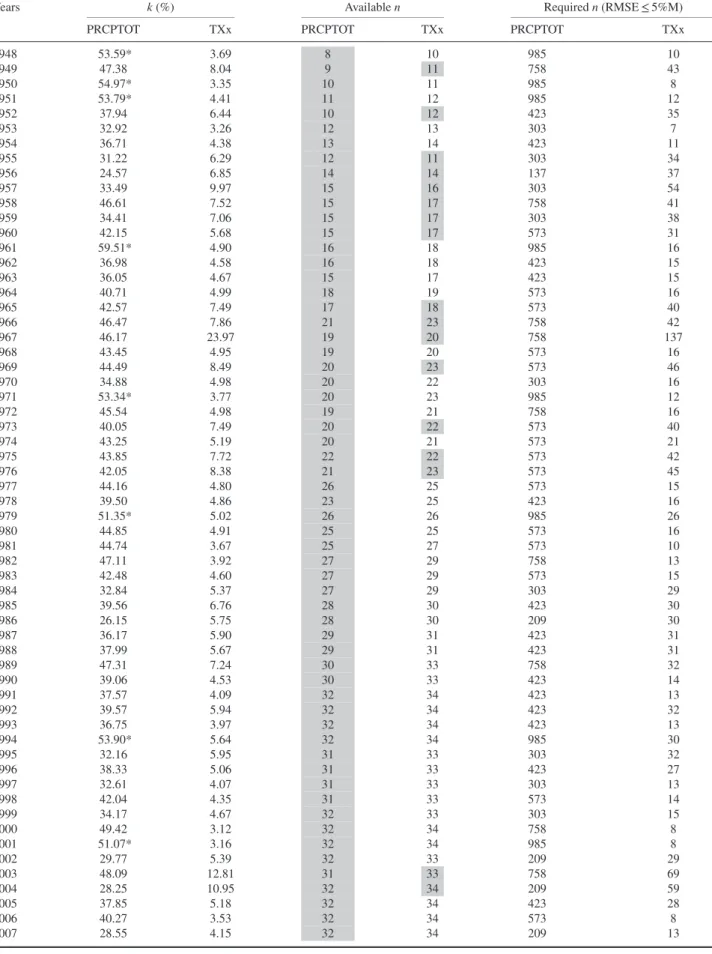
it as a data-scarce region. The minimum number (50) of data required for accurate and precise variogram estimation is not met with the current and maximally available number of data (Journel and Huijbregts, 1978; Webster and Oliver, 1992, 2001). Figure 1(a) represents the geographical location of Bangladesh with the distribution of currently active meteorological stations (data locations). During the study period of 1948–2007, there is a gradual increase in the number of data (n) for precipitation and temperature, i.e. from 8 to 32 and from 10 to 34, respectively (Figure 1(b)). This indicates that data scarcity was more critical at earlier periods, leading to more inaccurate and imprecise surfaces for those time steps.

To provide readers with a better understanding of data scarcity in the region, the area of interpolation for each of the available 34 data locations in 2007 is presented in Figure 1(c) with their corresponding Voronoi polygons. Each data location influences

the interpolation of an average area of 4 340 km2_{. Conforming to}

the number of data locations available, the area of interpolation influenced by each data location varies temporally. In 1948, when the number of available data is minimal (8), the interpolation

area that is influenced by each data location is approximately

18 000 km2_{on average.}

3. Materials and methods

The daily precipitation and temperature data from the avail-able meteorological stations in Bangladesh in a 60 years’ time series (1948–2007) were used in this study. Two annual cli-mate indices, the annual total precipitation in wet days (PRCP-TOT) and the yearly maximum value of the daily maximum temperatures (TXx), were computed. These indices are recom-mended by the joint CCl/CLIVAR/JCOMM Expert Team on Cli-mate Change Detection and Indices (ETCCDI) (Peterson et al., 2001; Frich et al., 2002) and allow analysis of climatic changes in Bangladesh (Bhowmik, 2012, 2013). A thorough quality con-trol has been performed on the raw data before computation of the indices. The ‘RClimdex’ routine (Peterson et al., 2001) was executed for the quality control and indices computation. Thus, PRCPTOT and TXx values were obtained for 8–32 and 10–34 data locations, respectively, for the 1948–2007 period. Detailed formulation of the indices and quality control procedures can be found in Zhang and Yang (2004), Bhowmik (2012, 2013) and Bhowmik and Cabral (2013).

The representativeness of the climate indices of their cor-responding climatic field were quantified by the regional co-efficient of variation (k, expressed in terms of a percentage) at each time step (Searlsa, 1964; Vangela, 1996). The k statistic is a measure of dispersion or deviation in the data from the mean.

A priori based knowledge indicates that high dispersion in the

climate indices of a region at a particular time step depicts low

representativeness of the indices. When k is> 50% the indices’

mean is not representative of the corresponding climatic field (Kelley, 2007; Belle, 2008; Lynch and Kim, 2010; Afonso and Nunes, 2011). Accordingly, in the context of this study, a set of

data was considered with null representativeness if k was> 50%.

In contrast, the values of the k statistic close to zero depict high representativeness of the data for the corresponding climatic field (Kelley, 2007; Belle, 2008; Lynch and Kim, 2010).

Since there is a functional relationship among the number of data (n), k and accuracy and precision of statistical estimation, the required n for obtaining satisfactorily accurate and precise interpolated surfaces under prevailing k was estimated and com-pared to the available n (Kelley, 2007; Lynch and Kim, 2010). Generally, spatial interpolation is accepted to be satisfactorily accurate and precise when the root mean square error (RMSE) of

the interpolated values is≤ 5% of the regional mean of observed

values (Kyriakidis et al., 2001; Carrera-Hernández and Gaskin, 2007; Durão et al., 2010). Therefore, the criterion for satisfac-tory accuracy and precision of spatial interpolation was set as

RMSE≤ 5% of the regional indices mean. This allowed

iden-tifying whether the available n was adequate for satisfactorily accurate and precise spatial interpolation. Details of this compu-tation and formulation are available in Kelley (2007) and Lynch and Kim (2010).

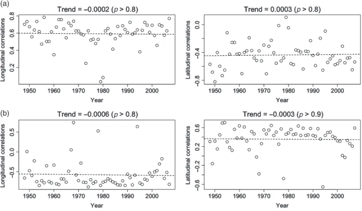
In the next step, the persistence of spatial structure of the indices during the study period was assessed as changes in spa-tial structure strongly affect the accuracy and precision of spaspa-tial interpolation (Kravchenko, 2003). This was done because neither the available n, nor k, took spatial structure of the indices into account, i.e. a random spatial shuffling of the indices over space changed neither the n nor the k. In order to identify spatial struc-ture, spatial correlations of the indices in the longitudinal and latitudinal gradients were computed. Thereafter, the statistical

(a)

(b) (c)

Figure 1. (a) Geographical location of Bangladesh and the spatial distribution of the 34 meteorological stations that are currently active, (b) increasing number of the data locations for precipitation [n(Precipitation)] (top) and temperature [n(Temperature)] (bottom) during 1948–2007, trend (slope) values with statistical significance are presented and (c) Voronoi polygons depicting the area of influence of each of the currently active 34 data

significance of trends in the spatial correlations during the study period was analysed to check the persistence of spatial structure. The nugget and sill ratios (nugget:sill) of three pooled variograms that were taken from Bhowmik (2012) were computed to identify the strength of spatial structure and its changes in three succes-sive periods: 1948–1975, 1976–1992 and 1993–2007 (Kerry and Oliver, 2008). The pooled variograms allowed for precise variogram estimation in response to a few number of data per time step (Isaaks and Srivastava, 1988; Atkinson and Tate, 2000). The Universal Kriging (UK) model (Caruso and Quarta, 1998; Christakos, 2001) was applied for spatial interpolation as this model has proven to be the most appropriate for interpolating PRCPTOT and TXx in Bangladesh (Bhowmik, 2012). The pooled variogram (Bivand et al., 2008) parameters for three suc-cessive periods: 1948–1972, 1973–1992 and 1993–2007, taken from Bhowmik (2012), were used in the UK model. Details of the UK spatial interpolation of the indices, variogram model param-eters and spatial trend paramparam-eters are available in Bhowmik (2012). The UK interpolation was performed using the ‘gstat’ package (Pebesma, 2004) in the R program (R Core Team, 2013). The assessment of accuracy and precision of spatial interpola-tion is based on the deviainterpola-tion of the interpolated values from the observed values, which can be measured through leave-one-out cross-validation (Seaman, 1983; Willmott, 1984). Different error statistics can be computed from cross-validation that indicates the deviation of the interpolated climate indices from their corre-sponding climatic field values (Seaman, 1983; Willmott, 1984). Four frequently used error statistics were computed (Dirks et al., 1998; Chiles and Delfiner, 1999): (1) root mean square error (RMSE), (2) mean absolute error (MAE), (3) systematic root mean square error (RMSEs) and (4) unsystematic root mean square error (RMSEu). The RMSE is the common measure of accuracy and precision of spatial interpolation. The MAE is an updated and preferred version of mean error that is less sen-sitive to extreme values, and evaluates the interpolation bias. Values of MAE close to zero indicate unbiased predictions. The RMSEs assesses whether the interpolation model errors are pre-dictable, whereas the RMSEu identifies those errors that are not predictable mathematically. Higher values of these error statis-tics indicate lower accuracy and precision of spatial interpolation. Detailed formulation of these error statistics can be found in Will-mott (1984). The cross-validation and computation of the error statistics were performed using the ‘gstat’ (Pebesma, 2004) and ‘hydroGOF’ (Zambrano-Bigiarini, 2011) packages in the R pro-gram (R Core Team, 2013). As an exploratory test, the statistical significance of trends in k and in the four error statistics was investigated for the study period.

Next, the relationship of the error statistics with the available n and computed k were analysed separately and compared to iden-tify which of the n and k had more (and significant) effect on the accuracy and precision of spatial interpolation. Before checking these relationships, the relationship between n and k was verified as n and k affect each other, i.e. a higher number of observations entails a higher representativeness of data (Kelley, 2007; Lynch and Kim, 2010). For such a purpose, in a first step, the effect of the available n on k was evaluated. The bivariate normality in the available n and k was tested using the Henze–Zirkler’s Multivariate Normality Test (Henze and Zirkler, 1990) using the ‘MVN’ package of R (Korkmaz, 2013), as recommended by Far-rell et al. (2007) and Mecklin and Mundfrom (2005). Since the n

and k statistics were significantly (p< 0.001) well fitted

accord-ing to the bivariate normal distribution, a simple linear regression model was fitted with the available n as predictor of k. In a sec-ond step, a generalized linear model with the ‘Poisson’ family

was fitted with k as predictor of the available n, since the avail-able n were count data (Sheskin, 2003). Afterwards, the residuals of both models were extracted as these residuals obliterate the effects of the available n and k on each other.

In the final stage, the bivariate normality in the residuals of the n and k models, paired separately with each of the four error statistics, were tested according to previous studies (Henze and Zirkler, 1990). Consequently, four simple linear regression els were independently fitted to the residuals of the two mod-els, to predict the four spatial interpolation error statistics of each index (PRCPTOT and TXx). The percentage of variabil-ity in the response variables (error statistics of both the indices) explained by the residuals of n and k was evaluated by the

adjusted co-efficient of determination (R2_{) and through the}

sta-tistical significance (p< 0.05) of their corresponding regression

parameters. This enabled identification of the effect of n and k on the error statistics and their comparison when n and k were independent of each other. Both the simple linear regressions and generalized linear models were fitted in the R program (R Core Team, 2013).

4. Results

An average k of 41% was observed for PRCPTOT resulting from a range of 24.57–59.51% whereas for TXx the average k was 6.2% with a range of 3.26–23.97% (Table 1). In eight tempo-ral steps, the PRCPTOT data showed null representativeness as

k was> 50%, and in 24 time steps they were less

representa-tive (40%≤ k ≤ 50%). As none of these cases was observed for

TXx, the TXx data were mostly representative of the climatic field, whereas PRCPTOT data were unrepresentative. In fact, for PRCPTOT, the number of available data did not meet the require-ment for obtaining satisfactory accuracy and precision of spatial interpolation according to the computed k in any of the time steps. On the contrary, in 43 time steps out of 60 (72%), the available n of TXx data met the requirement for satisfactory accuracy and precision (Table 1). These results conformed to the computed RMSE of the UK spatial interpolation of the indices (Table 1; Table S2, Supporting Information). For PRCPTOT, in all the time

steps, the RMSE was> 5% of the regional mean under prevailing

k, whereas for TXx, except for the time steps when the required n for satisfactory accuracy and precision were not met the RMSE

was< 5% of the regional mean (Tables S1, S2).

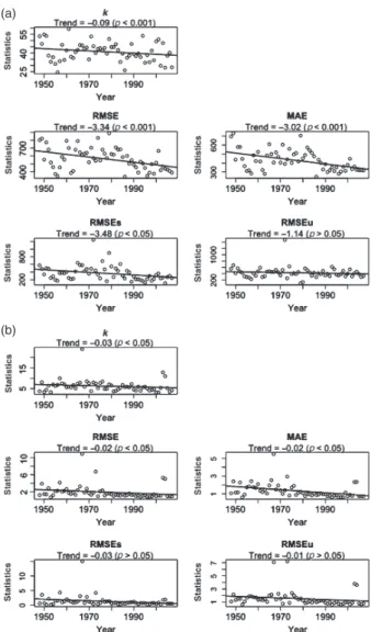
The trends in the k and the error statistics during the study period showed a pattern associated with the trends in the available

n (Figures 1 and 2). The k and the error statistics showed

decreasing trend with increasing n meaning the PRCPTOT and TXx data showed increasing representativeness and their spatial interpolation showed increasing accuracy and precision during the study period. The trends were mostly statistically significant at p< 0.05.

The trends in the spatial correlations of the indices in the lon-gitudinal and latitudinal gradients were statistically insignificant and minimal, depicting the persistence of their spatial struc-ture (Figure 3). The nugget:sill for the pooled variograms of the 1948–1975, 1976–1992 and 1993–2007 periods of the PRCP-TOT and TXx were 0.38, 0.33, 0.35 and 0.1, 0.18, 0.16, respec-tively. Therefore, there is a moderate and strong spatial structure in the PRCPTOT and TXx, respectively, which were also per-sistent among the pooled periods. These results depicted that the persistent spatial structure of the PRCPTOT and the TXx were not affecting the accuracy and precision of the spatial interpolation of the indices apart from the change in the available

Table 1. Computed representativeness (k – co-efficient of variation) of the climate indices (PRCPTOT and TXx) at every time step (years) of the study period and corresponding available and required number of data (n) according to the measured k (Kelley, 2007; Lynch and Kim, 2010) for

satisfactorily accurate and precise [root mean square error (RMSE)≤ 5% of the regional mean of the indices (M)] spatial interpolation.

Years k (%) Available n Required n (RMSE≤ 5%M)

PRCPTOT TXx PRCPTOT TXx PRCPTOT TXx

1948 53.59* 3.69 8 10 985 10 1949 47.38 8.04 9 11 758 43 1950 54.97* 3.35 10 11 985 8 1951 53.79* 4.41 11 12 985 12 1952 37.94 6.44 10 12 423 35 1953 32.92 3.26 12 13 303 7 1954 36.71 4.38 13 14 423 11 1955 31.22 6.29 12 11 303 34 1956 24.57 6.85 14 14 137 37 1957 33.49 9.97 15 16 303 54 1958 46.61 7.52 15 17 758 41 1959 34.41 7.06 15 17 303 38 1960 42.15 5.68 15 17 573 31 1961 59.51* 4.90 16 18 985 16 1962 36.98 4.58 16 18 423 15 1963 36.05 4.67 15 17 423 15 1964 40.71 4.99 18 19 573 16 1965 42.57 7.49 17 18 573 40 1966 46.47 7.86 21 23 758 42 1967 46.17 23.97 19 20 758 137 1968 43.45 4.95 19 20 573 16 1969 44.49 8.49 20 23 573 46 1970 34.88 4.98 20 22 303 16 1971 53.34* 3.77 20 23 985 12 1972 45.54 4.98 19 21 758 16 1973 40.05 7.49 20 22 573 40 1974 43.25 5.19 20 21 573 21 1975 43.85 7.72 22 22 573 42 1976 42.05 8.38 21 23 573 45 1977 44.16 4.80 26 25 573 15 1978 39.50 4.86 23 25 423 16 1979 51.35* 5.02 26 26 985 26 1980 44.85 4.91 25 25 573 16 1981 44.74 3.67 25 27 573 10 1982 47.11 3.92 27 29 758 13 1983 42.48 4.60 27 29 573 15 1984 32.84 5.37 27 29 303 29 1985 39.56 6.76 28 30 423 30 1986 26.15 5.75 28 30 209 30 1987 36.17 5.90 29 31 423 31 1988 37.99 5.67 29 31 423 31 1989 47.31 7.24 30 33 758 32 1990 39.06 4.53 30 33 423 14 1991 37.57 4.09 32 34 423 13 1992 39.57 5.94 32 34 423 32 1993 36.75 3.97 32 34 423 13 1994 53.90* 5.64 32 34 985 30 1995 32.16 5.95 31 33 303 32 1996 38.33 5.06 31 33 423 27 1997 32.61 4.07 31 33 303 13 1998 42.04 4.35 31 33 573 14 1999 34.17 4.67 32 33 303 15 2000 49.42 3.12 32 34 758 8 2001 51.07* 3.16 32 34 985 8 2002 29.77 5.39 32 33 209 29 2003 48.09 12.81 31 33 758 69 2004 28.25 10.95 32 34 209 59 2005 37.85 5.18 32 34 423 28 2006 40.27 3.53 32 34 573 8 2007 28.55 4.15 32 34 209 13

*k exceeding the threshold of 50%, thus showing null representativeness.

(a)

(b)

Figure 2. Trends in the representativeness (k – co-efficient of variation) and the error statistics (RMSE, root mean square error; MAE, mean abso-lute error; RMSEs, systematic root mean square error; RMSEu, unsys-tematic root mean square error) computed through the cross-validation of the spatial interpolation of the (a) annual total precipitation in wet days (PRCPTOT) and (b) yearly maximum value of the daily maximum tem-peratures (TXx) indices. The trend (slope) values with their statistical

significances (p) are presented.

The available n and k could significantly explain each other although the explained variability and slopes were very low (Table 2). The results of the fitted simple linear regression mod-els depict that the slopes of the error statistics with the chang-ing k are much higher than with the changchang-ing n (Table 3). The slopes with the changing k are all statistically significant, whereas with the changing n they were statistically insignif-icant. Moreover, k explains 39.67% [78.16%] of the variabil-ity in the RMSE of spatial interpolation of PRCPTOT [TXx] and the corresponding regression parameters are statistically sig-nificant (Table 3). Complementarily, n explains only 13.56% [3.38%] of the variability in the RMSE of PRCPTOT [TXx]; thus its regression parameters are not statistically significant (Table 3). On average, the k explains much higher variabil-ity of the error statistics than the available n and showed sta-tistical significance when n and k were independent of each other (Table 3). More than 70% of the variability in each of the error statistics of TXx is explained by k except for RMSEu (Table 3).

5. Discussion and conclusion

The influence of the number of data on the accuracy and pre-cision of spatial interpolation has been discussed as of utmost importance (Sluiter, 2009; Li and Heap, 2011) and several studies have highlighted the consequences of scarce data (e.g. Goovaerts, 2000; Bhowmik and Cabral, 2011; Bhowmik, 2012, 2013; Bhowmik and Costa, 2012). By contrast, the present study shows that the representativeness of the data, i.e. the variability of the climate phenomenon, is more crucial than the number of data for ensuring accuracy and precision. The regression analyses showed that the number of data is weakly related to the accuracy and precision, whereas their representativeness has a significant relation. Therefore, accurate and precise spatial interpolation could be accomplished for the yearly maximum value of the daily maximum temperatures (TXx) at almost all time steps, but in none of the time steps for annual total pre-cipitation in wet days (PRCPTOT) in Bangladesh, even though the numbers of available data are comparable (Table 1; Tables S1, S2). Moreover, the number of observations (n) explained a small percentage of the variability in accuracy and precision, whereas their representativeness, measured by the co-efficient of variation (k), explained most of it (Table 3). Thus, the repre-sentativeness of the data proved to be a better predictor of the accuracy and precision of spatial interpolation than the number of observations. These results conform to the influence of data representativeness on the accuracy and precision of statisti-cal estimation (Hewitson and Crane, 2005; Hill and Lewicki, 2006). The variability of the systematic root mean square error (RMSEs) and the unsystematic root mean square error (RMSEu) explained by k for PRCPTOT was somehow lower than for the other indices (Table 3). Nevertheless, the variability in these error statistics of PRCPTOT explained by k was much higher than that explained by n.

It is important to note that some parameters may not be sta-tistically significant, though they are of practical interest for regression analysis. Even if sometimes the change component is present, it may not be detected by statistical tests at a satis-factory significance level (Yue and Hashino, 2003; Radziejewski and Kundzewicz, 2004; Basistha et al., 2007). Although these authors considered other climatic variables, it can be argued that the number of observations is somehow affecting the accu-racy and precision of spatial interpolation of the indices, despite not being significant in general, and that its influence is con-siderably lower than the representativeness. Moreover, a small but significant variability could be explained in the number of observations by their representativeness, and vice versa. Thus, in regions with abundant data, satisfactory accuracy and preci-sion might be obtained without taking their representativeness into account (Dirks et al., 1998; Kyriakidis et al., 2001; Kast-elec and Košmelj, 2002; Diodato, 2005; Hijmans et al., 2005; Haberlandt, 2007). However, in data-scarce regions, where the accuracy and precision of spatial interpolation have been ques-tioned due to few data (Goovaerts, 2000; Carrera-Hernández and Gaskin, 2007; Bhowmik and Costa, 2012), the representative-ness of the climate data should be treated as highly important. Particularly in the spatial interpolation of precipitation, which is a highly variable spatial phenomenon, satisfactory represen-tativeness should be ensured in order to obtain satisfactory accu-racy and precision (Tabios and Salas, 1985; Phillips et al., 1992; Hewitson and Crane, 2005).

The required number of PRCPTOT data that were estimated following the methods of Kelley (2007) and Lynch and Kim (2010), for obtaining satisfactory accuracy and precision in spatial interpolation, were substantially high (more than 700) in

(a)

(b)

Figure 3. Trends in the spatial correlations in the longitudinal and latitudinal gradients of the (a) annual total precipitation in wet days (PRCPTOT) and (b) yearly maximum value of the daily maximum temperatures (TXx) indices during 1948–2007. The trend (slope) values with their statistical

significances (p) are presented.

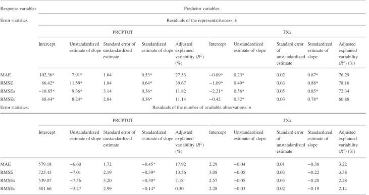
Table 2. Co-efficients of the simple linear regression model and generalized linear models with Poisson family fitted to the representativeness (k – co-efficient of variation) and the available number of data (n) of the climate indices (PRCPTOT and TXx), respectively, where the n and k were, respectively, the predictors. The intercept, unstandardized estimate of slope, standard error of unstandardized estimate, standardized estimate

of slope and the adjusted explained variability of the models are presented with the co-efficients’ statistical significance (p< 0.05).

Response variables Predictor variables

Number of available observations: n

PRCPTOT TXx Intercept Unstandardized estimate of slope Standard error of unstandardized estimate Standardized estimate of slope Adjusted explained variability (R2_{) (%)} Intercept Unstandardized estimate of slope Standard error of unstandardized estimate Standardized estimate of slope Adjusted explained variability (R2_{) (%)} Representativeness: k (simple linear regression model) 45.38* −0.19* 0.13 −0.19* 1.91 7.54* −0.05* 0.05 −0.14* 0.31 Representativeness: k PRCPTOT TXx Intercept Unstandardized estimate of slope Standard error of unstandardized estimate Standardized estimate of slope Adjusted explained variability (R2₎ (%) Intercept Unstandardized estimate of slope Standard error of unstandardized estimate Standardized estimate of slope Adjusted explained variability (R2_{) (%)} Number of available observations: n (generalized linear model with the Poisson family)

3.47* −0008* 0.004 −0008* 4.44 3.30* −0.02* 0.009 −0.006* 1.98

Table 3. Co-efficients of the simple linear regression models fitted to the error statistics (RMSE, root mean square error; MAE, mean absolute error; RMSEs, systematic root mean square error; RMSEu, unsystematic root mean square error), where the representativeness (k – co-efficient of variation) and the available number of data (n) of the climate indices (PRCPTOT and TXx) were separately the predictors. The intercept, unstandardized estimate of slope, standard error of unstandardized estimate, standardized estimate of slope and the adjusted explained variability of the linear

regression models are presented with the co-efficients’ statistical significance (p< 0.05).

Response variables Predictor variables

Error statistics Residuals of the representativeness: k

PRCPTOT TXx Intercept Unstandardized estimate of slope Standard error of unstandardized estimate Standardized estimate of slope Adjusted explained variability (R2₎ (%) Intercept Unstandardized estimate of slope Standard error of unstandardized estimate Standardized estimate of slope Adjusted explained variability (R2_{) (%)} MAE 102.36* 7.91* 1.64 0.53* 27.53 −0.09* 0.23* 0.02 0.87* 76.29 RMSE 86.42* 11.59* 1.84 0.64* 39.67 −1.09* 0.49* 0.03 0.88* 78.16 RMSEs −18.85* 9.36* 3.14 0.36* 11.82 −2.21* 0.56* 0.05 0.85* 72.34 RMSEu 88.44* 8.24* 2.84 0.36* 11.14 −0.42 0.32* 0.03 0.78* 60.88 Error statistics: Residuals of the number of available observations: n

PRCPTOT TXx Intercept Unstandardized estimate of slope Standard error of unstandardized estimate Standardized estimate of slope Adjusted explained variability (R2₎ (%) Intercept Unstandardized estimate of slope Standard error of unstandardized estimate Standardized estimate of slope Adjusted explained variability (R2_{) (%)} MAE 579.18 −6.60 1.72 −0.45* 17.92 2.29 −0.04 0.01 −0.38 3.22 RMSE 723.43 −7.01 2.19 −0.39* 13.56 3.08 −0.05 0.03 −0.22 3.38 RMSEs 539.07 −7.56 3.20 −0.30* 7.18 2.57 −0.05 0.03 −0.20 2.28 RMSEu 501.66 −3.27 2.99 −0.14* 0.30 2.28 −0.03 0.02 −0.19 2.14 *Statistically significant at p≤ 0.05.

the presence of little and null representativeness. The estimation procedure followed a very narrow confidence interval, which might lead to these high values. In addition, practically, the

con-dition of root mean square error (RMSE)≤ 5% of regional mean

of the indices (M) might not be appropriate for developing coun-tries, considering their economic and technological constraints (Table 1). Hence, research is required for setting appropriate con-fidence interval and conditions for satisfactory accuracy and pre-cision of climate spatial interpolation in those regions. Moreover, precipitation is likely to be influenced by several other meteoro-logical and terrain parameters within the study regions (Hewitson and Crane, 2005). Therefore, redistribution of rain-gauges in space, such that the point observations can be representative of a continuous surface, may also decrease the variability and thus increase representativeness, apart from increasing the number of observations. As available n showed little predictability for the k (Table 2), other meteorological and terrain parameters should be taken into account in regions with highly variable precipitation.

The effect of small amounts of data and low data density depends mostly on the variability of the attribute being analysed, the spatial configuration of the data and the size and characteris-tics of the study region (Journel and Huijbregts, 1978). There-fore, it is highly recommended that the rain-gauge networks are increased or redistributed in data-scarce regions such as Bangladesh for achieving satisfactory representativeness. Given that the estimated number of rain-gauges is too high to be obtained, or they could not be redistributed properly, future stud-ies could compute the response surfaces of precipitation for rep-resentative bounded continuum (Hewitson and Crane, 2005) of synoptic states with the point observations being spot samples of a representative continuous surface. Such representative pre-cipitation sub-regions can be established based on other meteo-rological parameters and terrain characteristics, and the distance

decay relationship can be established based on the corresponding covariance function between homogenous observations.

The spatial structure of climatic variables often affects the accuracy and precision of their spatial interpolation, though it was not observed in this study (Kravchenko, 2003; Figure 3). If significant influence of spatial structure is observed, spatial correlation parameters in longitudinal and latitudinal gradients should be fitted as predictors of accuracy and precision of spatial interpolation. Thus, the effects of these predictors should also be obliterated while analyzing the impacts of the available number of observations and representativeness on the accuracy of the spatial interpolation of climate data.

Given the significantly low representativeness of the data, accu-rate and precise PRCPTOT surfaces for Bangladesh are not pro-ducible for the 1948–2007 period. Nevertheless, a few studies have computed precipitation surfaces despite the data scarcity and low representativeness in Bangladesh (Shahid, 2009, 2010; Bhowmik, 2012, 2013), and in other data-scarce regions (Suhaila and Jemain, 2011). This study showed that these surfaces are not satisfactorily accurate and precise, thus they do not pro-vide enough detail and should be used cautiously in comprehen-sive research. In contrast, the regional temperature surfaces, as computed by Bhowmik (2012, 2013) and Bhowmik and Cabral (2013) are satisfactorily accurate and precise and can be used in further research.

Acknowledgements

This study has been carried out within the framework of the Euro-pean Commission, Erasmus Mundus Programme; project no. 2007-0064. The authors thank two anonymous reviewers for their constructive comments, which led to an improved manuscript. The authors declare no conflict of interest.

Supporting information

The following material is available as part of the online article:

Table S1.Regional mean (M) error statistics (RMSE – Root Mean Square Error, MAE – Mean Absolute Error, RMSEs –

Systematic Root Mean Square Error, RMSEu –

Unsystematic Root Mean Square Error) and the percentage RMSE of M (RMSE/M) computed from Universal Kriging cross-validation at every time step (year) for the PRCPTOT index.

Table S2.Regional mean (M) error statistics (RMSE – Root Mean Square Error, MAE – Mean Absolute Error, RMSEs –

Systematic Root Mean Square Error, RMSEu –

Unsystematic Root Mean Square Error) and the percentage RMSE of M (RMSE/M) computed from Universal Kriging cross-validation at every time step (year) for the TXx index.

References

Afonso A, Nunes C. 2011. Probabilidades e Estatística. Aplicações e Soluções em SPSS. Escolar Editora: Lisboa.

Atkinson PM, Tate NJ. 2000. Spatial scale problems and geosta-tistical solutions: a review. Prof. Geogr. 52(4): 607–623, DOI: 10.1111/0033-0124.00250.

Basistha A, Goel NK, Arya DS, Gangwar SK. 2007. Spatial pattern of trends in Indian sub-divisional rainfall. Jalv. Sam. 22: 47–57. Belle GV. 2008. Statistical Rules of Thumb, Vol. 2. John Wiley & Sons:

Hoboken, NJ.

Bhowmik AK. 2012. A comparison of Bangladesh climate surfaces from the geostatistical point of view. ISRN Meteorol. 2012, DOI: 10.5402/2012/353408.

Bhowmik AK. 2013. Temporal patterns of the two-dimensional spa-tial trends in summer temperature and monsoon precipitation of Bangladesh. ISRN Atmos. Sci. 2013, DOI: 10.1155/2013/148538. Bhowmik AK, Cabral P. 2011. Statistical evaluation of spatial

interpo-lation methods for small-sampled region: a case study of tempera-ture change phenomenon in Bangladesh. In Computational Science and Its Applications – ICCSA 2011: Lecture Notes in Computer Sci-ence, Mugante B, Gervasi O, Iglesias A, Taniar D, Apduhan BO (eds). Springer: Heidelberg; 44–59, DOI: 10.1007/978-3-642-21928-3_4. Bhowmik AK, Cabral P. 2013. Space-time variability of summer

tem-perature field over Bangladesh during 1948-2007. In Computational Science and Its Applications–ICCSA 2013: Lecture Notes in Com-puter Science, Murgante B, Misra S, Carlini M, Torre CM, Nguyen H, Taniar D, Apduhan BO, Gervasi O (eds). Springer: Berlin; 120–135, DOI: 10.1007/978-3-642-39649-6_9.

Bhowmik AK, Costa AC. 2012. A geostatistical approach to the seasonal precipitation effect on boro rice production in Bangladesh. Int. J. Geosci. 3(3): 443–462, DOI: 10.4236/ijg.2012.33048.

Bivand RS, Pebesma EJ, Gómez-Rubio V. 2008. Applied Spatial Data Analysis with R. Springer Science and Business Media, LLC: New York, NY.

Boer EPJ, De Beurs KM, Hartkamp AD. 2001. Kriging and thin plate splines for mapping climate variables. Int. J. Appl. Earth Obs. Geoinf. 3(2): 146–154, DOI: 10.1016/S0303-2434(01)85006-6.

Cai Y, Weihong Q, Song Y, Zhengmin L. 2010. Regional features of precipitation over Asia and summer extreme pre-cipitation over Southeast Asia and their associations with atmospheric–oceanic conditions. Meteorol. Atmos. Phys. 106: 57–73, DOI: 10.1007/s00703-009-0052-5.

Carrera-Hernández JJ, Gaskin SJ. 2007. Spatiotemporal analysis of daily precipitation and temperature in the Basin of Mexico. J. Hydrol. 336: 231–249, DOI: 10.1016/j.jhydrol.2006.12.021.

Caruso C, Quarta F. 1998. Interpolation methods comparison. Comput. Math. Appl. 35(12): 109–126, DOI: 10.1016/S0898-1221(98)00101-1.

Chiles J, Delfiner P. 1999. Geostatistics: Modeling Spatial Uncertainty. John Wiley & Sons: New York, NY, DOI: 10.1002/9780470316993. Christakos G. 2001. Modern Spatiotemporal Geostatistics. Oxford

Uni-versity Press: Oxford, UK.

Costa AC, Durão R, Pereira MJ, Soares A. 2008. Using stochas-tic space-time models to map extreme precipitation in southern

Portugal. Nat. Hazard Earth Syst. Sci. 8(4): 763–773, DOI: 10.5194/nhess-8-763-2008.

Diodato N. 2005. The influence of topographic co-variables on the spatial variability of precipitation over small regions of complex terrain. Int. J. Clim. 25(3): 351–363, DOI: 10.1002/joc.1131.

Dirks KN, Hay JE, Stow CD, Harris D. 1998. High-resolution studies of rainfall on Norfolk Island: Part II: interpolation of rainfall data. J. Hydrol. 208(3-4): 187–193, DOI: 10.1016/S0022-1694(98)00155-3. DMICCDMP – Disaster Management Information Center of

Compre-hensive Disaster Management Program. 2013. Bangladesh Meteo-rological Department. http://www.bmd.gov.bd/index.php (accessed 1 May 2013).

Dumolard P. 2007. Uncertainty from spatial sampling: a case study in the French Alps. In Spatial Interpolation for Climate Data. The Use of GIS in Climatology and Meteorology, Dobesch H, Dumolard P, Dyras I (eds). ISTE Ltd.: London; 57–70.

Durão R, Pereira MJ, Costa AC, Côrte-Real JM, Soares A. 2009. Indices of precipitation extremes in southern Portugal – a geostatis-tical approach. Nat. Hazard Earth Syst. Sci. 9(1): 241–250, DOI: 10.1002/joc.1999.

Durão R, Pereira MJ, Costa AC, Delgado J, del Barrio G, Soares A. 2010. Spatial-temporal dynamics of precipitation extremes in south-ern Portugal: a geostatistical assessment study. Int. J. Clim. 30(10): 1526–1537, DOI: 10.1002/joc.1999.

Farrell PJ, Salibian-Barrera M, Naczk K. 2007. On tests for multivariate normality and associated simulation studies. J. Stat. Comput. Simul. 77(12): 1065–1080, DOI: 10.1080/10629360600878449.

Frich P, Alexander LV, Della-Marta P, Gleason B, Haylock M, Klein Tank AMG, et al. 2002. Observed coherent changes in climatic extremes during the second half of the twentieth century. Clim. Res. 19: 193–212, DOI: 10.3354/cr019193.

Goovaerts P. 1997. Geostatistics for Natural Resources Evaluation. Oxford University Press: New York, NY.

Goovaerts P. 1998. Ordinary cokriging revisited. Math. Geosci. 30(1): 21–42, DOI: 10.1023/A:1021757104135.

Goovaerts P. 2000. Geostatistical approaches for incorporating elevation into the spatial interpolation of rainfall. J. Hydrol. 228: 113–129, DOI: 10.1016/S0022-1694(00)00144-X.

Haberlandt U. 2007. Geostatistical interpolation of hourly precipitation from rain gauges and radar for a large-scale extreme rainfall event. J. Hydrol. 332: 144–157, DOI: 10.1016/j.jhydrol.2006.06.028. Henze N, Zirkler B. 1990. A class of invariant consistent tests for

multivariate normality. Commun. Stat. Theory Methods 19(10): 3595–3617, DOI: 10.1080/03610929008830400.

Hewitson BC, Crane RG. 2005. Gridded area-averaged daily pre-cipitation via conditional interpolation. J. Clim. 18: 41–57, DOI: 10.1175/JCLI3246.1.

Hijmans RJ, Cameron SE, Parra JL, Jones PG, Jarvis A. 2005. Very high resolution interpolated climate surfaces for global land areas. Int. J. Clim. 25: 1965–1978, DOI: 10.1002/joc.1276.

Hill T, Lewicki P. 2006. Statistics: Methods and Applications: A Com-prehensive Reference for Science, Industry, and Data Mining. Stat-Soft: Tulsa, OK.

IPCC – Intergovernmental Panel on Climate Change. 2001. Climate Change 2001: Impacts, Adaptation and Vulnerability. Contribution of Working Group II to the Third Assessment Report of the Intergovern-mental Panel on Climate Change. Cambridge University Press: Cam-bridge.

IPCC – Intergovernmental Panel on Climate Change. 2007. Climate Change 2007: Impacts, Adaptation and Vulnerability. Contribution of Working Group II to the Fourth Assessment Report of the Intergovern-mental Panel on Climate Change, Parry ML, Canziani OF, Palutikof JP, van der Linden PJ, Hanson CE (eds). Cambridge University Press: Cambridge, UK.

Isaaks EH, Srivastava RM. 1988. Spatial continuity measures for prob-abilistic and deterministic geostatistics. Math. Geol. 20(4): 313–341, DOI: 10.1007/BF00892982.

Journel AG, Huijbregts CJ. 1978. Mining Geostatistics. Academic Press: New York, NY.

Karmakar S, Shrestha ML. 2000. Recent climate change in Bangladesh. Proceedings of South Asian Association for Regional Cooperation (SAARC) Seminar on Climate Variability in the South Asian Region and Its Impacts, September, Dhaka.

Kastelec D, Košmelj K. 2002. Spatial interpolation of mean yearly precipitation using Universal Kriging. In Developments in Statis-tics, Mrvar A, Ferligoj A (eds). Metodološki zvezki: Heidelberg; 149–162.

Kelley K. 2007. Sample size planning for the coefficient of variation from the accuracy in parameter estimation approach. Behav. Res. Methods 39(4): 755–766, DOI: 10.3758/BF03192966.

Kerry R, Oliver MA. 2008. Determining nugget:sill ratios of standard-ized variograms from aerial photographs to krige sparse soil data. Precis. Agric. 9(1-2): 33–56.

Klein Tank AMG, Peterson TC, Quadir DA. 2006. Changes in daily temperature and precipitation extremes in central and south Asia. J. Geophys. Res. 111(D16): D16105.

Korkmaz S. 2013. MVN: multivariate normality tests. http://cran. r-project.org/web/packages/MVN/index.html (accessed 10 July 2013).

Kravchenko AN. 2003. Influence of spatial structure on accuracy of interpolation methods. Soil Sci. Soc. Am. J. 67(5): 1564–1571. Kyriakidis PC, Kim J, Miller NL. 2001. Geostatistical mapping of

pre-cipitation from rain gauge data using atmospheric and terrain charac-teristics. J. Climatol. 40(11): 1855–1877, DOI: 10.1175/1520-0450 (2001)040<1855:GMOPFR>2.0.CO;2.

Li J, Heap AD. 2011. A review of comparative studies of spatial interpolation methods in environmental sciences: performance and impact factors. Ecol. Inform. 6: 228–241, DOI: 10.1016/j.ecoinf. 2010.12.003.

Lloyd CD. 2005. Assessing the effect of integrating elevation data into the estimation of monthly precipitation in Great Britain. J. Hydrol. 308: 128–150, DOI: 10.1016/j.jhydrol.2004.10.026.

Lynch RM, Kim B. 2010. Sample size, the margin of error and the coefficient of variation. InterStat 4.

Mecklin CJ, Mundfrom DJ. 2005. A Monte Carlo comparison of the type I and type II error rates of tests of multivariate normality. J. Stat. Comput. Simul. 75(2): 93–107, DOI: 10.1080/009496504200019 3233.

Mia NM. 2003. Variations of temperature of Bangladesh. Proceedings of South Asian Association for Regional Cooperation (SAARC) Seminar on Climate Variability in the South Asian Region and Its Impacts, 10–12 December 2002, Dhaka.

Pebesma E. 2004. Multivariable geostatistics in S: the gstat package. Comput. Geosci. 30: 683–691, DOI: 10.1016/j.cageo.2004.03.012. Peterson TC, Folland C, Gruza G, Hogg W, Mokssit A, Plummer

N. 2001. Report on the activities of the Working Group on Cli-mate Change Detection and Related Rapporteurs 1998–2001. Report WCDMP-47, WMO-TD 1071, World Meteorological Organization: Geneva.

Phillips DL, Dolph J, Marks D. 1992. A comparison of geostatisti-cal procedures for spatial analysis of precipitations in mountain-ous terrain. Agric. For. Meteorol. 58: 119–141, DOI: 10.1016/0168-1923(92)90114-J.

R Core Team. 2013. R: A Language and Environment for Statis-tical Computing. R Foundation for StatisStatis-tical Computing: Vienna http://www.R-project.org (accessed 1 July 2013).

Radziejewski M, Kundzewicz ZW. 2004. Detectability of changes in hydrological records. Hydrol. Sci. J. 49: 39–51, DOI: 10.1623/hysj.49.1.39.54002.

Seaman RS. 1983. Objective analysis accuracies of statistical interpo-lation and successive correction schemes. Aust. Meteorol. Mag. 31: 225–240.

Searlsa DT. 1964. The utilization of a known coefficient of variation in the estimation procedure. J. Am. Stat. Assoc. 59(308): 1225–1226, DOI: 10.1080/01621459.1964.10480765.

Shahid S. 2009. Spatio-temporal variability of rainfall over Bangladesh during the time period 1969-2003. APJAS 45(3): 375–389.

Shahid S. 2010. Trends in extreme rainfall events of Bangladesh. Theor. Appl. Climatol. 104: 489–499, DOI: 10.1007/s00704-010-0363-y. Sheskin DJ. 2003. Handbook of Parametric and Nonparametric

Statisti-cal Procedures. Chapman & Hall/CRC: Boca Raton, FL.

Sluiter R. 2009. Interpolation methods for climate data – literature review. KNMI, R&D Information and Observation Technology, KNMI Intern Rapport, IR 2009-04, Version 1.0, De Bilt.

Suhaila J, Jemain AA. 2011. Spatial analysis of daily rainfall intensity and concentration index in Peninsular Malaysia. Theor. Appl. Clima-tol. 108(1-2): 235–245.

Tabios GQ, Salas JD. 1985. A comparative analysis of techniques for spatial interpolation of precipitation. J. Am. Water Resour. Assoc. 21(3): 365–380, DOI: 10.1111/j.1752-1688.1985.tb00147.x. Tveito OE. 2007. The developments in spatialization of meteorological

and climatological elements. In Spatial Interpolation for Climate Data. The Use of GIS in Climatology and Meteorology, Dobesch H, Dumolard P, Dyras I (eds). ISTE Ltd.: London; 73–86.

Vangela MG. 1996. Confidence intervals for a normal coefficient of variation. Am. Stat. 50(1): 21–26.

Wagner PD, Fiener P, Wilken F, Kumar S, Schneider K. 2012. Comparison and evaluation of spatial interpolation schemes for daily rainfall in data scarce regions. J. Hydrol. 464-465: 388–400.

Webster R, Oliver MA. 1992. Sample adequately to estimate variograms of soil properties. J. Soil Sci. 43(1): 177–192.

Webster R, Oliver MA. 2001. Geostatistics for Environmental Scientists. John Wiley & Sons: Chichester.

Weisse AK, Bois P. 2001. Topographic effects on statistical characteristics of heavy rainfall and mapping in the French Alps. J. Clim. 40(4): 720–740, DOI: 10.1175/1520-0450(2001) 040<0720:TEOSCO>2.0.CO;2.

Willmott CJ. 1984. On the evaluation of model performance in physical geography. In Spatial Statistics and Models, Gaile GL, Willmott CJ (eds). 443–460. Springer: AK Houten, Netherlands.

Yue S, Hashino M. 2003. Long term trends of annual and monthly precipitation in Japan. J. Am. Water Resour. Assoc. 39: 587–596, DOI: 10.1111/j.1752-1688.2003.tb03677.x.

Zambrano-Bigiarini M. 2011. hydroGOF: goodness-of-fit functions for comparison of simulated and observed hydrological time series, R package version 0.3-7. http://cran.r-project.org/web/ packages/hydroGOF/ (accessed 1 June 2013).

Zhang X, Yang F. 2004. RClimDex (1.0) User Guide. Climate Research Branch Environment Canada: Downsview, ON.