The Peso Problem
Literature Review
Trabalho Final na modalidade de Dissertação apresentado à Universidade Católica Portuguesa
para obtenção do grau de mestre em Finanças
por
Vasco Rodrigues Quintino
sob orientação do ProfessorGonçalo Faria
Católica Porto Business School 04/2018
iii
v
Abstract
Peso Problem situations represent a market reaction prior to abrupt events, that although expected to occur may actually never happen. They so
correspond to an anticipation of the event by market participants, their behaviour being biased by the expectation of the abrupt event. The “Peso Problem” concept originated in the currency market, but the situation is transversal to any asset in the market place. This thesis aims to give a
perspective of how Peso Problem situations affect asset pricing behaviour in the currency, equity, bond and derivatives markets. Acknowledging that a biased market data behaviour can result from people’s attitudes, behavioural finance forwards an alternative to the traditional Efficient Market Hypothesis point of view for the Peso Problem and similar market data behaviours.
Keywords: Peso-Problem; Biased market data; Future uncertainty; Equity markets; Bond markets; Derivatives markets; Behavioural finances.
vii
Contents:
Abstract ... v
Contents ... vii
Figure and Table Index ... ix
Introduction ... 1
Chapter 1 The Peso Problem in the Currency Market ... 5
1.1 Forecasts ... 6
1.2 Forward-Premium Puzzle ... 8
Chapter 2 The Peso Problem in the Bond Market ... 13
Chapter 3 The Peso Problem in the Equity Market ... 19
3.1 Peso Problem, the Equity Premium Puzzle and the Survivorship Bias ... 20
3.2 Regime Switching Models ... 28
Chapter 4 The Peso Problem in the Derivatives Markets ... 31
Chapter 5 The Peso Problem and Econometric Issues... 35
Chapter 6 The Peso Problem and Behavioural Finance ... 39
6.1 The Prospect Theory ... 40
6.1.1 The Wheighting Function ... 43
6.1.2 The Value Function ... 44
6.2 Behavioural Finance and the Peso Problem ... 46
Concluding Remarks ... 49
References ... 55
ix
Figure and Table Index:
Figure 1 – The actual and hypothetical relationship between the one-month forward rate and
the spot rate between the Canadian and the U.S. dollar. Source: Hopper (1994) ... 9
Figure 2 – U.S. Yield Term Structure from 1929 to 2014 ... 16 Figure 3 – The graph on the left illustrates the timing of the regime switch computed by Lewis
(1991), and the graph on the right illustrates the two types of probabilities of the Peso Problem term of the yield term structure. Adapted from Lewis (1991). ... 18
Figure 4 – The implied (IV) and realized volatility (RV) of the options prices of the S&P 500, for
the period between 1996 to 2013. LTCM = Long-Term Capital Management Fund ... 21
Figure 5 – Annual average returns for 39 countries in the equity markets for the period between
1921 to 1996. Adapted from Jorion and Goetzmann (1999)... 24
Figure 6 – The Peso Problem Model (PPM) associated with losses of 15% (Panel A) and 10%
(Panel B). PPM measures the percentage differences in conditional probability of one-month index gross return below 0.85 and 0.9 under the option-implied and the index-return
conditional physical distribution. The shaded areas represent recession periods identified by the National Bureau of Economic Research (NBER). Adapted from Zhang and Zhou (2015). ... 27
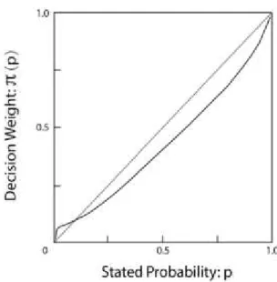
Figure 7 - The weighting function, showing the relationship between the decision weight and
the stated probability of the event. Adapted from Kahneman and Tversky (1979). ... 43
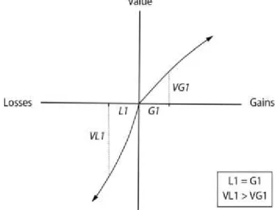
Figure 8 - The value function. The value attached to a similar amount of loss or gain, L1 and G1,
is higher for the loss (VL1) than for the gain (VG1). Adapted from Kahneman and Tversky (1979) and Thaler (2016) ... 45
Table 1. Experimental decision outcomes with positive and negative perspectives, illustrating
the violation of the risk aversion axiom of the expected utility theory. Adapted from Kahneman and Tversky (1979). N= 95. The percentage of respondents that selected each outcome is shown in brackets [ ]. ... 41
Table 2. Summary table mentioning relevant contributions from various authors to the study of
1
Introduction
Farmers protect their harvest, whenever they expect to have bad weather in upcoming days; Fishermen sell their fish in the market at the earliest hour because they expect to be the most lucrative timing; Athletes increase their training routine when they expect to face harder competitions; Companies issue equity to the market to raise capital for a project they except to be lucrative; Portfolio managers hedge their position when they expect higher risk. In all the above and many more examples, expectations matter and pervade in all the decisions made. Economy is a social science that studies the production, consumption and distribution of goods and services, aiming to explain how they work and their agents interact. Within economy, finance handles the creation, management and study of the components of financial systems, such as money, banking, credit, investments, assets and liabilities. Like farmers, athletes, fishermen, companies and governments, so financiers and economists decide accordingly to their future expectations, to anticipate the behaviour of the elements attached to their professions. Exchange rates, stocks, bonds and derivatives are examples of assets financiers deal with. Their values however, depend not only on the most likely future event but also on events less likely to occur. Incorporating these less likely events in assets pricing could make markets look flawed, even if they are not. Economists named this the “Peso-Problem”.
“Peso-Problem”, as the name implies, refers to a situation initially associated with the Mexican currency (Peso). The origin of the term is unknown, although
2
economists attribute it to Milton Friedman, when he commented about the differences in the currency rates between the US dollar and the peso (Sill, 2000). At the time, the exchange rate of the two currencies was fixed, as it had been since 1954, but there was a discrepancy between rates in the market. The interest rates on deposits in Mexican Banks was higher than in US Banks. At first, this could seem a flaw in financial markets but Friedman pointed out that the difference between interest rates could represent a possible devaluation of the peso, showing concerns towards the Mexican economy. Such discrepancy should disappear through the market efficiency theory, as investors would increasingly take advantage of it. Finally, in August 1976, when the peso was allowed to float against the dollar, it dropped 46%. Someone not aware of such potential devaluation of the Peso could interpret the market as inefficient since the rate had been fixed for 20 years. However, when investors recognised the event (the potential devaluation), the market expectations were proven to be correct. More generally, a “Peso Problem” arises whenever is considered the possibility that the occurrence of some infrequent event will affect asset prices. Such events are difficult, even impossible, to predict based on historical data (Sill, 2000).
The process of predicting possible outcomes of a response variable using present and past information of relevant explanatory variables is called a forecast. In our daily lives, we do this intuitively, but economists forecast using numerical models. While theoretical models try to obtain qualitative answers to the different implications of human behaviour, the economic agents, empirical models try to prove that these qualitative answers are plausible by applying them precise and numerical outcomes.
Fama (1965; 1970), was among the first to attempt to explain the formation of prices under a theory he called the Efficient Market Hypothesis (EMH). This theory
3
considers that markets are efficient, meaning that prices are a reflection of all the information available, any change being due to new information that enters the market. The information that is presented to the market, and consequently to the agents involved, is considered to be random, which means that any price change will also be random. Thus, price changes can be modelled as stochastic processes. The agents involved are also considered to act in a rational way with the information that is being presented to them.
Infrequent events, such as the peso devaluation, can influence market
expectations in a way that would make markets behave differently from the EMH. Most of the literature around the Peso Problem is related to the market anomalous behaviour at a specific moment, associating it with a failure of the EMH. Lewis (2007), nevertheless showed that this would only appear to be so if the problem was analysed in a short time frame, whereas if the data was brought to a longer time frame analysis, the theory could still hold. The extent to which an infrequent event in the market expectations can influence asset prices, is the motivation to study the Peso Problem. It began to be analysed in the currency market, but the concept is transversal to all financial assets. Examples of Peso Problem studies include, , Rogoff (1977) , Obstfeld (1987) and Lewis (2007), in the currency market; Lewis (1991), Sola and Driffill (1994), Evans and Lewis (1994) and Bekaert et al. (2001), in the bond market; Cecchetti et al. (1990), Rietz (1988), Evans (1998), Jorion and Goetzmann (1999), Veronesi (2004) , Ang et al. (2007), Zhang and Zhou (2015), in the equity market; Salant and Henderson (1978), in the gold market; Bondarenko (2003), in the derivatives market. Peso Problem formulations have been analyzed under the realm of the Efficient Market Hypothesis theory as well as under the Prospect theory in Behavioural Finance (Kliger and Levy 2009).
4
This thesis provides a literature review on the Peso Problem and how it has been analysed in the currency, equities, bonds and derivatives market. Chapter 1 focus on the Currency market and mentions the origin of the Peso Problem, how it influenced forecasts and why it was perceived as an anomaly. In Chapter 2, the Bond Market, the concept is brought to a more general analysis. In Chapter 3, in the Equity Market, the Peso Problem is related with the equity premium puzzle. Insurance techniques are also influenced by the Peso Problem, which are addressed in Chapter 4, on Derivatives market. In Chapter 5, is mentioned Peso Problem main inferences difficulties encounter by researchers. The concept is placed under the context of Behavioural Finances, in Chapter 6. The concluding remarks point to the benefits of the continuing study of the Peso Problem.
5
Chapter 1
The Peso Problem in the Currency Market
Smith (1776, in: Wilmott and Orrell, 2017) suggested that market behaviour could be explained by what is known as the law of demand and supply. This theory was criticized because of its lack of predictability in moments of market stress and The Efficient Market Hypothesis (EMH), developed by Fama (1965; 1970), would become the backbone of academic models used in risk analysis and much of the quantitative finance in general. However, in financial forecasting infrequent economical events still cannot be adequately foreseen by such numerical models.
Events such as the “Black-Monday” or the crisis of 2008, lead to debate if markets behave as suggested by Fama (1965; 1970). Both these crises showed that when asset prices depend on market expectations, the mere possibility of occurrence of an extreme event can have important repercussions. This was the reason that led economists to coin the term Peso Problem, in the 1970’s, when there were concerns regarding the valuation of the Mexican peso in relation to the US dollar. These concerns were being reflected in the higher returns investors could get from Mexican bonds when compared to US bonds, at a time when the rate between currencies was fixed, and so the returns should be similar. Such concerns, in general are nothing more than expectations about the future. In the financial markets, to delineate accurate future expectations about assets, when there is the possibility of occurrence of an event that is not well represented in the current and
6
past data (like the devaluation of the peso), can be a hard task to accomplish. Since asset prices embody financial market’s probabilities about possible future values of particular economic variables, they are sensitive to Peso Problems. So, which consequences can situations like the Peso Problem bring to forecasts?
1.1. Forecasts
Forecasts are valued as being good or bad accordingly to the errors they produce. These represent the differences between the expected (predicted) and realized (observed) values. If on average the model returns zero errors, then the expected values oscillate around the realized values, meaning the expected values were predicted without bias. On the contrary, the model is biased if the expected values are too high or too low for long periods of time.
Wars, recessions and political turmoil are examples under which forecasts and predictions could transmit biased results. As Obstfeld (1987) pointed out, one of the most puzzling aspects of the post 1973 floating exchange rate system was the inefficient predictive performance of forward exchange rates.
Like any forecast, forward contracts represent the expectations agents/investors have on how the market will react in the future, meaning on how the spot rate will behave. These models are supported by the EMH, which states that forecasts are correct on average, where positive returns will cancel the negative ones and no net extra returns will be generated. In this case, it means that the forward rate on average will be equal to the market’s expectation of what the spot rate will be when the contract expires. The forward rate will not present the exact value of the spot rate, in any given moment, but on average will approximate it. In some months, the forward will be higher and in others lower, making the forecasts unbiased, translating into an efficient market. This suggests no space for
7
profitability, although extra returns would appear randomly. Fama (1984), suggested a way of testing the market efficiency, by linear regressing the change in the spot rate on the forward premium:
∆𝑠𝑡+𝑘 = 𝛼 + 𝛽(𝑓𝑡− 𝑠𝑡) + 𝜖𝑡+𝑘 , (Eq. 1)
where ∆𝑠𝑡+𝑘 is the percentage depreciation (appreciation) of the exchange rate over
k periods and (𝑓𝑡− 𝑠𝑡) is the difference between the forward and the current spot
rate (forward premium).
The market would be efficient if the null hypothesis was confirmed, which according to Froot and Thaler (1990) would be that 𝛽 = 1 and 𝛼 = 0 meaning that the realized depreciation (appreciation) of the spot rate would equal the interest differential plus the error term 𝜖𝑡+𝑘. However, statistics show that the
forward-rates are not unbiased predictors of the future spot rate. Forward forward-rates tend to be too high or too low for extended periods of time, making it a biased predictor. As Froot and Thaler (1990) pointed out, most authors estimated 𝛽 to be less than zero, a few estimated it being positive, but none equal to the null hypothesis of 𝛽 = 1. This result was well shown by Evans and Lewis (1995), when they regressed the dollar exchange rate against the German Mark, British Pound and Japanese Yen (see the first column in Table from Annex 1).
The assumptions that the markets were efficient and expectations correct, were therefore questioned. Given the nature of the Peso Problem, the foreign exchange rate literature paid a good deal of attention to the potential role of Peso Problem in the so called Forward Premium Puzzle (Obstfeld, 1987).
8
1.2. Forward Premium Puzzle
The Peso Problem in the currency market is very much related to the biased behaviour of the forward rate in a short time horizon. This means that the Peso Problem impacts the forecast errors in short timeframe samples. The term small in this context refers to a sample with an unrepresentative number of regime sifts rather than the number of observations on returns, or even the time span of the data. However, Lewis (2007) demonstrated that this biased behaviour was only evident in a short time horizon, but no longer seen in an extended time window. This emphasized the fact that Peso Problems should not be seen has an inefficiency of the EMH (Lewis, 2007), but rather as a difficulty on making correct predictions of asset prices under market instability.
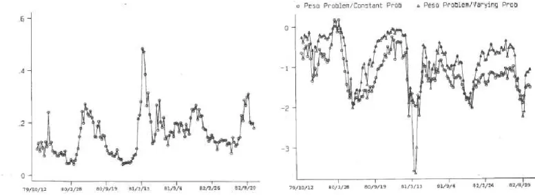
One example of the biased behaviour mentioned above can be seen in the study by Hopper (1994), relating the one-month forward and the one-month-ahead spot Canadian - U.S. dollar exchange rates from 1973 to 1993, illustrated in Figure 1. The left side of the figure shows the actual values, and the forward exchange rate tends to stay below the spot rate for extended periods when the spot rate is rising and to stay above the spot rate for extended periods when the spot rate is falling, meaning that the forward exchange rate is a biased predictor of the one-month ahead spot exchange rate. The right side of Figure 1 shows a projection of the null hypothesis mentioned before on how the forward and the spot exchange rates should behave according to the EMH (Hopper, 1994).
9
Figure 1 – The actual and hypothetical relationship between the one-month forward rate and the spot
rate between the Canadian and the U.S. dollar. Source: Hopper (1994).
However, some economists believe that there is an explanation for the biased pattern observed in the data, without discarding the idea that the market is efficient. They considered the Peso Problem as a way to explain such behaviour. If the exchange-markets expect that there is a possibility of the exchange rate to fall, until it actually does, the forward will remain below or above the spot rate, since the forward rate embodies the markets expectations. This was what happened during the 1970’s with the Mexican peso versus the US dollar rate. Rogoff (1977, in: Lewis, 2007) was the first to argue that the Peso Problem could be an explanation for the behaviour of the forward contracts. Without discarding the conventional rational assumptions of the EMH, Lewis (2007) gives the following examples to understand the effect that Peso Problem brings to exchange rates.
By using the relationship between the spot and the forward rate, 𝑠𝑡+1would
be the logarithm of the future spot rate (dollars per peso), at t+1, and 𝐹𝑡would be
the rate agreed at date t for delivery at t+1. The relation would be translated into the equation:
𝑠𝑡+1− 𝐹𝑡 = 𝑅𝑡+ 𝑈𝑡+1 (Eq. 2)
Where 𝑅𝑡 is the risk premium (difference between the actual spot and the
10
the spot rate, 𝑈𝑡+1= 𝑆𝑡+1− 𝐸𝑡 𝑆𝑡+1, where 𝐸𝑡 is the expectations created based on
the information at date t.
In the period 1954 to 1976, the spot peso exchange rate was fixed at 0.08 dollars per peso. Using this notion, 𝑆𝑡+1 was constant (named 𝑆0 hereafter).
However, what was observed in the market was a higher rate in holding peso deposits than dollar deposits, over the early 1970s. Implying that the forward agreed according to Equation 2 was smaller than the ex post spot rate (𝐹𝑡 < 𝑆0).
Meaning that 𝑆0− 𝐹𝑡 was systematically positive. Under the assumption of the
market’s efficiency (EMH) this should not hold true since it implies that the market’s forecast error 𝑆𝑡+1− 𝐸𝑡 𝑆𝑡+1 was being biased and serially correlated.
In August 1976, when the peso was allowed to float, it dropped to 0.05 dollars per peso, which resulted into a 46% decrease. If 𝑆1 represents this
devaluation, this could be translated into the relationship 𝑆1− 𝐹𝑡 = -46 per cent.
Lewis (2007) stated that this apparent paradox of the Mexican peso could be explained if one took account of this large negative observation summed to the large small positive observations over the early 1970s, which would result in a value close to zero. This would prove that the efficiency and the rational expectation assumptions were actually correct, holding the validity of the EMH reasoning.
Lizondo (1983), continued to study these forecast errors, admitting that traders indeed assumed rational expectations. He translated the expectations of the future spot rate into the equation:
11
Where 𝑝𝑡, is the market’s probability that the peso will be devalued to 𝑆1 at date
t+1. Therefore, as long as the rate would remain fixed at 𝑆0 , the forecast error
would be:
(Eq. 4)
Since the Mexican spot rate in the early 1970s was greater than the devalued rate, the initial spot rate 𝑆0 was greater than the anticipated rate if devaluations
were to occur, 𝑆1 ( 𝑆0> 𝑆1). This means that the ex post forecast errors were
systematically positive. The ex post bias in the forecast errors depended upon both the devaluation probability 𝑝𝑡, and the expected size of the fall in the exchange rate, 𝑆0 - 𝑆1. When the devaluation occurred this was a large negative observation
(1 − 𝑝𝑡)(𝑆1− 𝑆0).
In a sample with many observations of similar devaluations, forecast errors would be persistently positive between infrequent large negative observations. The frequent small positive forecast errors and the infrequent large negative forecast errors will tend to cancel each other out. Over a sufficient large sample of rare events, the forecast errors would roughly sum to zero, as implied by the rational expectations, linking the occurrence to the behaviour of values above and below to a mean in a normal distribution. However, the market appears to make persistent errors between discrete events, even though the forecasts will be unbiased in sufficiently large samples. Even in large samples, therefore, rational forecast errors with the Peso Problem may be serially correlated.
However, Evans and Lewis (1995) found that the Peso Problem was not enough to provide a full explanation for the biased results of the Forward Premium Puzzle, although it was economically relevant (see columns 3 and 4 of the Table in Annex 1). These authors rewrote β in Fama’s linear regression equation and added a third
12
term to the equation. This term represented the serial correlation of the forecast errors and the forward premium as perceived in a Peso Problem. By doing so, they would infer the influence of the Peso Problem. Columns (3) and (4) of the Table presented in Annex 1 illustrates their results. Column (3) indicates that the Fama coefficient may indeed be biased downward, by the presence of a Peso Problem. Their Monte Carlo Simulations in column (4) indicates to what extent peso problems may influence the standard deviation of the risk premium calculated in the previous regression. In the case of the Pound and the Mark, the peso problem influenced the standard deviation of the true risk premium about 20%. These results illustrate how the Peso Problem can affect coefficient estimates found in conventional regressions in small sample.
So far, the Peso Problem has been described as a single event and what implications it has on the forecasts made by market participants in small samples. This view is important but for predicting purposes may reveal to be insufficient. Another method that economists have used to model the Peso Problems is to consider that economy goes through changes in regimes (Evans, 1996), which lead to the development of the regime switching models.
13
Chapter 2
The Peso Problem in the Bond Market
Regime switching models evaluate to which extent repeated but infrequent discrete shifts in the distribution of shocks hitting the economy could induce Peso Problem behaviour in asset prices. This is an important distinction in respect to the previous approach, because if an event is repeated, even infrequently, there is the possibility of describing it statistically. In general, regimes represent different environments. The goal is to try to understand how the components within each regime behave. In other words, as Sill (2000) pointed out, the key concept for such approach is that in one regime the disturbances (unpredictable events) to the economy are different from what they are in another regime.
Situations such as the Peso Problem, where expectations point towards the occurrence of discrete events, could be affected by variables like interest rates, inflation or output growth differently in each regime.
This concept, although simple and realistic, taking into account the cycles that the economy is known to go through, is not simple to model. The process of how the future uncertainty is set in the model creates difficulties. As Evans (1996) pointed out, the majority of the approaches that try to model the economy through different regimes are usually nonlinear, making inferences difficult to accept.
14
The first application of a switching model to a fundamental based asset pricing model appeared in Hamilton (1988, in: Evans, 1996) and was related to the U.S. yield term structure from 1962 to 1978.
The usual approach researchers used to incorporate a Peso Problem into a switching model was to produce two different regimes under which the assets fundamentals would output different results. One represented the regime under which the agents expected a change and the other under which the economy remained as before, no changes occurring. However, the analysis can only be conceptualized under a Peso Problem situation, when the market participants attribute different probabilities to each regime. Only then the market participants are considered to attribute a change from one period to the next.
Hamilton (1979, in: Evans, 1996) placed a complex set of rational expectation restrictions on the behaviour between short and long rates, which led him to find that the component of the Peso Problem was almost absent in his analysis. However, this was shown by Evans (1996) to be due to similar regime probabilities.
Sola and Driffill (1994) arrived to different conclusions. Differently from Hamilton (1979, in: Evans 1996), these authors considered switches in the yield spread when there were changes in the process of short term rate. This implied that the spread between rates in their switching model would follow stationary I (1) processes, even when long and short rates followed non-stationary I (0) processes. This allowed them to estimate the same timing of a regime switch as Hamilton (1988, in: Evans 1996), but with very different probabilities. In this case, it was considered that agents do not ignore the component of a Peso Problem.
15
These two studies illustrate that Peso Problems could be relevant or not, depending on the specifications chosen for the model. Such specifications will be discussed in Chapter 5.
The results reached by Sola and Driffill (1994) were comparable to those obtained by Lewis (1991) and by Evans and Lewis (1994). Lewis (1991), estimated that the existence of a Peso Problem was an important component in the analysis, not only for investment strategies but also to follow monetary policies in the economy. The approach she used in her analysis is detailed below.
Figure 2 illustrates the U.S. yield term structure between Treasury Bills of 3-months and Treasury Bonds of 10 years, from 1927 to 2014 (87 years). The graph shows the evolution of interest rates of these two bonds, and it can be noticed that the volatility of the short-term interest rates was higher than that of the long-term (standard deviation of 0.032 versus 0.027, respectively). One of the reasons behind this result is the fact that short term yields tend to be more influenced by the monetary policies set by central banks, than the longer-term yields, which causes shorter yields to behave closer to the economic cycles, than long term interest rates, in agreement with Sill (1996). This author reported that the strength of the correlation between output growth and interest rates tends to decline as the maturity of the bonds increases. This means that there is pro-cyclical behaviour in shorter yields than in longer ones (Sill, 1996).
16
However, when the amount of money supply is higher than the real income growth, inflation raises and the interest rates would not co-vary with the output growth anymore. In fact, during the great inflation observed in the U.S. economy in the 80’s, short term interest rates grew higher than longer maturities to almost 20% (cf. Figure 2), triggering the unemployment rate in the U.S. economy to 10.8%. According to Lewis (1991), this large spread between interest rates occurred due to the non-borrowed reserves (NBR) policy implemented by the Federal Reserve Bank (FRB) at the time. On the attempt to explain the U.S. term structure of interest rates, Lewis (1991) considered the spread between rates as a Peso Problem situation, as Sola and Driffill (1994) did, and analysed it as a signal of an anticipation of a future regime and policy change.
Lewis (1991) addressed the issue of whether a market anticipation of a switch in the monetary policy could systematically affect the ex post returns on longer term bonds relative to short term interest rates. To do so, Lewis (1991) considered an investment strategy in a longer maturity bond relative to rolling over the investment in a shorter maturity for successive periods.
17
As already stated in Peso Problems situations, when the market expects a discrete change in policy that does not materialize for some time, these expectations will induce forecast errors that are systematically mistaken ex post. By investing in the longer bond as long as interest rates followed regime 1 (NBR) ex post, the probability of switching to regime 2 would systematically generate a bias behaviour in the forecasts implicit in long rates. If the market believed that the interest rates would be lower when it changed to regime 2 than under regime 1, the Peso Problem term (expected returns and probabilities of regime 2) in the yield term structure equation, would on average be negative over that period. Thus, if market participants expect that the shorter rates would be lower than longer ones, this Peso Problem effect is going to result into a systematic decline in the returns on long bonds relative to short bonds, until the regime changes.
As stated before, for the analysis to be contextualized into a Peso Problem, Lewis (1991) used a constant probability method and a time varying one. These probabilities would update upon informational variables, for which Lewis (1991) decided to use the actual bond rates. Figure 3 plots both the estimated timing of a regime change (on the left side) and the Peso Problem term of the yield term structure equation (on the right side). It shows that the constant and the varying probability methods presented a similar pattern, although the time-varying probability estimate induced greater variation on the pick of the short-term interest rates (1979 to 1981, cf. Figure 2). Both varied more when a change in regime was expected (cf. Figure 3). After 1981 the monetary policies changed, causing a decrease in the interest rates of both bonds, especially in the short-term ones due to their higher sensitivity to these policies (cf. Figure 2).
18
So, the Peso Problem not only was shown to be a relevant component in investment strategies upon achieving excess returns in longer term bonds from an anticipation of a regime shift but also proved to be an important factor (specially the time-varying estimates) for following the political pressures on the FRB for the NBR policy.
The work of Lewis (1991) demonstrated that a Peso Problem situation was relevant in the bond market. Such estimates could also be brought to other fields in finance, as will be shown in the next Chapters.
Figure 3 – The graph on the left illustrates the timing of the regime switch computed by Lewis (1991), and the
graph on the right illustrates the two types of probabilities of the Peso Problem term of the yield term structure. Adapted from Lewis (1991).
19
Chapter 3
The Peso Problem in the Equity Market
Asset prices, such as stocks, depend on future dividend payments. A standard model to attribute price to stocks, such as the Discounted Dividend Model (Williams, 2013), takes into account the future dividends the stock will pay to the holder. When the prospects about the state of the economy are good, variables such as employment, real output, investments and consumption, all increase as well as the dividends. When this perception changes or the economy goes through a rough path, the variables mentioned above decrease and that will also be reflected in the dividends. The stock prices act accordingly: higher dividends foster higher prices and lower dividends promote lower prices. There are however unusual situations, when the dividends grow in a direction opposite to the state of the economy, so that during good regimes dividends can be low, while the opposite holds, for bad regimes. Because of such irregularity, investors cannot be certain on how the state of the economy will be, based upon the return on dividends. This makes the analysis of Peso Problem occurrences in stock prices complex.
Investors act based on their assessment towards the reward they earn relative to the risks they assume. Risk and the way it is considered in investments, is then an important variable in the analysis of how the equities and bond markets react to Peso Problem situations.
20
Risks and rewards throughout the evolution of quantitative finance were modelled differently, although under the same perspective of earning higher returns with higher risks and aiming to best possible inference future uncertainty.
However, in the literature related to the equity and bond markets, there are still anomalies in the market place not fully understood, of which the Equity Premium Puzzle. On the attempt to solve this puzzle, some models look to the Peso Problem as a possible solution for this phenomenon.
3.1. Peso Problem, the Equity Premium Puzzle and the
Survivorship Bias
The concept of equity premium puzzle was introduced by Mehra and Prescott (1985). The term came with the demonstration that the commonly used economic model, Consumption Capital Asset Pricing Model, CCAPM, was incapable of accounting for the observed high rates of return on stocks when compared to those of short-term bonds (T-bills). Those authors applied this model to a set of historical prices ranging from 1889 to 1978. As in a previous version of this model, the Capital Asset Pricing Model, CAPM, investors would have a utility function, however measured by the marginal utility of consumption, and a relative risk averse coefficient, A. According to their research, A would range between 0 and 10. However, when applying to that time series of historical returns values of A within this range, Mehra and Prescott (1985) concluded that this pricing model could not account for the total annual average equity premium. In order to capture the real results, they would have to apply much higher values to the risk coefficient A, between 30 and 40. These authors considered such risk coefficients to be implausibly high and named this situation the Equity Premium Puzzle.
21
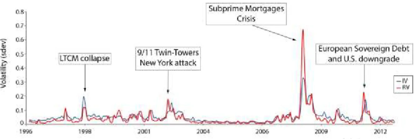
One way to understand the equity premium puzzle is to plot the implied volatility (IV) of options prices against time, IV showing a correlation of 0.62 with the equity premium, according to Graham and Campbell (2007). Figure 4 illustrates the evolution between 1996 and 2013 of the implied (IV) and the realized (RV) volatility of options prices of Standard and Poor 500. IV and RV were calculated according to Faria and Kosowski (2016), from whom this data was obtained.
Figure 4 clearly shows the high volatility of both measures during the study period, the implied volatility being higher than the realized in 81% of the time series. A proxy that could be used to represent the equity premium of investors compensation, would be the difference between the two, given the correlation mentioned before. The implied volatility imposed by option prices can be used to assess the market sentiment/expectation of future instability. The events plotted in Figure 4 represent moments of high social and financial instability which were also moments when investors got higher premia for the risks they were bearing, which can be noticed by the larger differences between the two volatility measures.
Figure 4 – The implied (IV) and realized volatility (RV) of the options prices of the S&P 500, for
22
The literature around the Peso Problem related to the equity premium puzzle, as in the currency market, looks to bias in the data, by measuring to which extent a peso component drives the prices to show a continuous tendency (bias), to the point that these expectations are met/materialized. A hypothesis that helps to put this into perspective in the equity market is known as the survivorship bias. The hypothesis states that when investors are worried about the possibility of occurrence of a drastic event, which although not happened, might have, should receive the respective compensation for such risks. Among others, the literature around the Peso Problem and the survivorship bias is discussed by Rietz (1988) and Jorion and Goetzmann (1999).
Rietz (1988), by modifying the assumptions in the CCPAM model, allowed investors to make the assumption that large sudden drops in the market could occur during recessions. The consumption growth rate during such times would not match exactly the stock dividends, which had not been considered by Mehra and Prescott (1985). In situations where the future expectations indicated abrupt decreases both in consumption and in dividends, investors would mainly hold stocks, instead of bonds, if they were compensated by a high average equity premium. As Siegel and Thaler (1997) pointed out, this alternative explanation to the equity premium puzzle looks at the investors as rationally worried about a small chance of an economic catastrophe, which, though it had not happened, might have. The Peso Problem, when investors consider the possibility of an event that so far did not happen, stand out as the possible empirical modification introduced in Rietz (1988) work. He stated that if the CCAPM included the possibility of abrupt market drops both in consumption and in dividends during recessions, the values of the equity premium presented in Mehra and Prescott (1985) could be accounted for.
23
Jorion and Goetzmann (1999) also considered Peso Problem occurrences as a potential explanation to the equity premium puzzle. They analyzed a large range of equity markets in the period 1921-1996 from 39 countries, including those that experienced functioning interruptions of the stock market due to tragic events (wars, hyperinflation…), such as in France, Finland, Germany, Japan, Portugal and others, and those that did not, such as the US market. For this sample of 39 countries, the highest returns were generated in the United States, Sweden and Canada, where no interruptions due to external events occurred, with 4.32, 4.29 and 3.19 percent annual returns respectively (Figure 5). On the contrary, in countries such as Germany or Japan, that suffered interruptions in their stock market due to war events, the markets fell 72 and 95 percent respectively, which contributed to lower annual returns (cf. Figure 5). Jorion and Goetzmann (1999) identified 25 events that caused market interruptions, due to drastic events in history, most of which during the second world war and due to invasions to Poland, Denmark, Norway, Netherlands, Belgium, France and Greece. Other cases related to the civil war in Spain during 1936 to 1940, political turmoil or religion causes, as in Portugal in 1974 and Egypt in 1962, respectively.
24
Figure 5 – Annual average returns for 39 countries in the equity markets for the period between
1921 to 1996. Adapted from Jorion and Goetzmann (1999).
The peso problem comes as a possible answer to the discrepancy among countries, since Jorion and Goetzmann (1999) pondered the possibility that based on the historical drastic events, investors considered that if other stock markets were suspended or even terminated for long periods of time due to infrequent events, the same could happen to the US market. With almost a century of uninterrupted history, the remote possibility of a market failure is not without reason. Once more, the Peso Problem appears to give an explanation for the failure of the expectations implied in the models, which consider the ex-ante distribution of endogenous variables to be a good approximation to the ex-post distribution. In a market where the risk and reward almost have a symbiotic relationship with each other, in situations where the expectations of the future indicate scenarios where large losses are considered to be plausible, investors will demand higher returns for the assumed risks.
In the context of the Peso Problem, the survivorship bias hypothesis helps to understand the core problem of research around the equity market and the puzzle of the equity premium. Siegel and Thaler (1997) pointed out that this hypothesis is
25
very hard to test and can be discredited, since the data acquired from Mehra and Prescott (1985) did contain an economic catastrophe, namely the Great Depression, from 1929 to 1933, when stocks lost about 80 percent of their value. Such controversies around the survivorship bias hypothesis and the Peso Problem come from the lack of empirical support in both these works. However, a recent paper developed by Zhang and Zhou (2015), provided some empirical evidence related with such hypothesis in the sense that the high premia demanded by investors could be in fact due to the risks they were prepared to take.
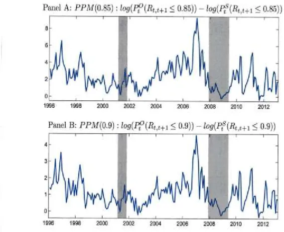
The model by Zhang and Zhou (2015) was based on data derived from option prices and index returns from the period between 1996 to 2013. On the attempt to measure the sentiment/expectations of market participants, the purpose of the study was to compute the difference between the perceived risk expected by investors’ ante of an infrequent event, with the actual realized index returns ex-post. Authors wished to observe to which extent a Peso Problem component could contribute for the discrepancies in the two sets of values. The Peso Problem model they developed was expressed in the percentage difference between two conditional probabilities of two implied physical distributions. The two distributions made reference to an option-implied conditional physical distribution, derived by option prices, and an index-return implied physical distribution, derived by an index of returns. Physical in this sense means that there was a risk premium attached to each distributions. The two conditional probabilities represent each distribution (options and index) to be inferior to 0.85 and 0.9 (0.85 and 0.9 representing 15% and 10% loss, respectively). Since the options and the index are related to the S&P500 index, this will allow comparing the results obtained by Zhang and Zhou (2015), with the risk premia illustrated in Figure 4.
26
Zhang and Zhou (2015) main findings are illustrated in Figure 6, showing that the Peso Problem component was cyclical, outputting higher values during expansions and market booms and lower during recessions. The recession periods included the Twin-Towers collapse in 2001, the subprime mortgage crisis in 2008 and the European sovereign debt in 2011, the last one not shaded in Figure 6.
This behavior is supportive of the Peso Problem hypothesis. This means that the gap between the ex-ante perceived risk and the ex-post realized risk will narrow and vanish if large losses expected by investors have eventually occurred. These results coincide with the risk premia expressed in Figure 4, in the sense that the moments of higher instability in markets are the same as the moments when the model by Zhang and Zhou (2015) showed the lowest values.
27
These two analyses indicate that Peso Problem components could be of value to model an anticipation of an abrupt market change. This is shown by the fact that the perceived expectations made by market participants are not without reason, since when abrupt events do materialize (the subprime mortgage crisis and the European sovereign debt), the Peso component almost vanishes and the risks to which the markets are exposed, increase (cf. Figures 4 and 6). The cyclical behaviour of Peso Problems, showed by Zhang and Zhou (2015), contributes to the incentive of using regime switching models, as in the currency market, to further
Figure 6 – The Peso Problem Model (PPM) associated with losses of 15% (Panel A) and 10% (Panel B).
PPM measures the percentage differences in conditional probability of one-month index gross return below 0.85 and 0.9 under the option-implied and the index-return conditional physical distribution. The shaded areas represent recession periods identified by the National Bureau of Economic Research (NBER). Adapted from Zhang and Zhou (2015).
28
test whether a Peso Problem component is relevant or not to understand the behaviour of the equity market.
3.2 Regime Switching Models
Under the perspective that the economy goes through varying regimes, the essence of these models is to test whether or not a Peso Problem component is relevant on the variables chosen for the model. In the equity market, stock prices depend upon the dividends paid to investors, so the first aspect that is important to analyze is if this variable is affected by the Peso Problem.
Evans (1998), based on the dividend ratio model developed by Campbell and Shiller (1989), examined the maximum likelihood of the predictability of dividend growth between two regimes (0 and 1). Evans (1998) applied an annual series of stock prices and dividends of the S&P 500 from 1871 to 1987, to a number of estimates (Annex 2). The Peso Problem component is expressed in the estimates α (z) and β (z). They show how the predictability of dividend growth varies across regimes. Based on the values of the estimate α (z), market participants could predict switches in the dividend growth under regime 1, since it shows that past dividend growth is a useful predictor of its future, but not under regime 0 (confirm the first column of the table in Annex 2). However, the analysis would only be contextualized under a Peso Problem if market participants associate different probabilities to the forecasts of dividends growth across regimes. Only then, would a regime switch be implied from one period to the next. By looking at the estimates of λ (1) and λ (0), market participants did attribute different probabilities to each regime, the probability under regime 1 being approximately 10% and 1% in regime 0 (cf. Annex 2).
29
To assess more precisely the results from these estimates, Evans (1998) examined if his predictability in the dividend growth across regimes, would influence stock returns. To do so, Evans (1998) added a stock return variable to his switching model of dividend growth and studied the t-statistics of these estimates, by applying Monte Carlo simulations on two different regressions. The null hypothesis would be confirmed if their regression coefficients (a1 and b1, Annex 2) were equal to 0. If such hypothesis was confirmed, the variations in returns would not be predictable based on the dividend growth and there would be no point of analyzing a Peso Problem effect on the expectations of the market participants. Evans (1998) however only found a single case where he would not reject the null hypothesis (confirm table in Annex 2), meaning that the Peso Problem component would be valuable studying on the equity market, in specific to try to solve the equity premium puzzle.
However, as in the currency market, the inference of a Peso Problem influence in the expectations of market participants, depends upon the conditions under which uncertainty about the process driving future fundamentals is set. Following the work of Hamilton (1988; 1989, in Evans 1996), numerous switching specifications have been used to characterize regime switching in various applications. Evans (1996) enumerated a few, which used a component of a Peso Problem, namely the model developed by Cecchetti et al. (1990 in Evans 1996). Their switching model tries to explain the behavior of the equity returns by using estimates of consumption and dividends prices. Instead of using the concept of a standard equilibrium pricing model, which implies that market expectations of future variables will affect all the values of the current variables, Cecchetti et al. (1990 in Evans 1996) decided that such restriction would only affect the present value stock returns but not the consumption levels. This would imply that the
30
systematic forecast errors in small samples, which are characteristic of Peso Problems as illustrated in Chapter 1, would only be observable in the stock returns, but not in the estimates of consumption. This discrepancy of the influence of Peso Problem in these two estimates, makes the use of this component irrelevant for the analysis. Because of these different variations on how the future uncertainty can be characterized, inferences regarding the influence of the Peso Problem in regime switching models had not been fully successful, as indicated by Evans (1996).
Even so, Veronesi (2004) pointed out that the Peso Problem component is an important subject to analyze. He argued that the eventuality of a bad event could affect investors’ expectations in other ways from just generating higher returns ex-post as perceived in the equity premium puzzle. He exploited the ex-ex-post behavior of stock returns using a model that attributed a very small probability that the economy could enter a very long recession. Under this assumption, the Peso Problem could be the cause for further implications besides just a high realized equity premium. Such anomalies could include excess volatility1, asymmetric
volatility reaction to good and bad news and higher volatility during recessions2.
Nevertheless, regarding the different opinions, the main aspect these results indicate, is that in periods were a negative future is expected, following events such as those indicated in Figure 4, the behaviour of the market is more volatile than in any other moment and more difficulty to predict. As a response to this difficulty, insurance techniques were developed in finances, and these will be addressed in Chapter 4.
1 The excess volatility makes reference to the excess behavior the price of a stock has, related to changes in
dividends, according to Shiller (1981) and LeRoY and Porter (1981).
31
Chapter 4
The Peso Problem in the Derivatives Market
The use of derivatives grew enormously in the past 40 years, mostly because they provided investors with trading opportunities that otherwise would not be available. One of the benefits of derivatives is the variety of payoffs that are provided by them, due to the fact that returns can be gained from any desirable pattern the data presents. Recessions or expansions can be profitable. For that reason, investors can speculate, hedge or arbitrage in the market through the use of these assets. During periods of future uncertainty, such as in Peso Problems situations, these securities could provide insurances that other assets cannot. Such demand could create an attractive market to operate. In specific, selling unhedged out-of-the-money (OTM) put options of the S&P500 was particularly profitable in the period of 1987 to 2000. Due to the fact they were overpriced, such high returns became a puzzling phenomenon to many economists (Bondarenko, 2003).
While it is clear that options traders will sell OTM puts when properly rewarded for bearing substantial risks, it is much less clear what their normal risk compensation should be. These levels of risk premiums depend upon which equilibrium model is used. Models such as the CAPM or the Rubinstein (1976),
32
found the amount of compensation asked by the sellers to be too high for the risk premiums accounted for (Bondarenko, 2003). However any modification applied to new models can prove to be difficult to be acceptable.
Bondarenko (2003) based on the assumptions that part of the investment in put options is related to a hedging strategy against abrupt downturn changes in the future, Bondarenko (2003) used the expectations implied in the Peso Problem to find a solution for the anomaly. However, the resolution of such anomaly was developed around a nonstandard equilibrium model, which considered a similar approach to the Peso Problem as Cecchetti et al. (1990) in the equity market.
Following standard equilibrium models, in the beginning of the contract the models assume a set of conditions. These are based on the assumptions that markets are efficient and all the information presented to the agents is efficiently reflected in the prices, making the behaviour of the data unbiased. In the derivatives market, these conditions make reference to the set of pre-commitment assumptions at the beginning of the contract, expressed in the estimates of the pricing kernel. For periods when the observed values in the market appear to be biased, such as in Peso Problems, as long as there is a pre-commitment to an initial pricing kernel throughout the contract, put options returns would appear constantly overpriced, rejecting the assumptions of the Efficient Market Hypothesis, implied in models such as the CAPM and the Rubinstein (1976).
The conditions Bondarenko (2003) applied in his work tried to relax the initial commitments used by standard models, by adopting risk neutral probabilities (which would not invalidate the martingale behaviour implied by the EMH). These probabilities allow to attribute a price to derivatives based only on their final expected payoff. Using this approach, the previous rejections of the pricing kernel
33
during the maturity of the contract would be avoided. In other words, the pricing kernels throughout the contract would be path independent, and so the model would not contain forecast errors serially correlated, avoiding the characteristic situation of a Peso Problem. Every test and hypothesis would be applied for the maturity of the contract. If introducing in the model specific assumptions characteristic of a Peso Problem, and obtaining low returns of put options, then the anomaly would be solved and the model would hold. However, for the 144 inferences studied by Bondarenko (2003), this was strongly rejected. This implies that the equilibrium model he used could not explain the overpriced put options, even when allowing the pricing kernel component to be flexible, as Cecchetti et al. (1990) used in the equity market. Due to the rejections of his analysis, one of Bondarenko’s (2003) suggestions was: if a model account for a not fully rational behaviour by investors towards risk, it could be a helpful modification to analyse the anomaly. Such suggestion will be addressed in more detail in Chapter 6.
As Evans (1996) mentioned for both the equity and derivatives market, when the conditions implied in the pricing kernel avoid biased behaviours, the peso component for the subject under study would not appear to be relevant for the analysis. So, independently of the market to which the Peso Problem component is applied to, it may be or not a relevant component to explain the observed market outputs depending on how the conditions of future fundamentals are set in the models. This is one of the reasons why is easy to find so many studies around the Peso Problem being empirically analysed.
Besides the mentioned conditions that models needed to fulfil, Evans (1996) pointed out that most of them are highly nonlinear, making inferences regarding the Peso Problem difficult to be acceptable. Bellow it will be addressed the main
34
difficulties researchers may face when deciding to use a Peso Problem approach in numerical models.
35
Chapter 5
The Peso Problem and Econometric Issues
The presence of a Peso Problem can complicate inferences about the behaviour of asset prices in samples spanning a short timeframe. This is due to the bias behaviour of the forecast errors which the EMH does not support. According to this theory, these forecast errors should have mean zero with finite variances, making them unbiased. As long as there is uncertainty about the future variables, as in a Peso Problem situation, these forecast errors would be biased and may appear correlated with the ex ante information when viewed ex post. However, this biased behaviour, although considered abnormal, is seen as an anticipation made by market participants of a regime change. In the currency market this was materialized by the devaluation of the Mexican Peso in 1976, in relation to the US Dollar. Such potential anticipation makes the analysis of Peso Problems compelling to study. However, once this behaviour is recognized, the researcher is faced with two problems.
The first one concerns the sample size. According to Evans (1996), the extent to which biased behaviours can be found in a particular sample of forecast errors, depends upon the frequency of regime shifts in the sample. This means that, if the sample only contains the regime in which this anticipation does not materialize, the sample properties will remain biased. Alternatively, when the sample does
36
contain different regimes, the forecast errors will inherit a combination of different properties. If the anticipation of a regime shift does materialize, then the sample will have a mean close to zero and the forecast errors will appear uncorrelated with the ex ante information when viewed ex post. Under these circumstances the sample will display the conventional rational expectations properties implied by the EMH. Thus, there is the consensus that the presence of a Peso Problem can only impact the forecast errors made by market participants in small samples, not showing the different regimes. That is why the use of models which can properly represent regime sifts in the data, are more useful to analyse the Peso Problem. The second problem faced by researchers when analysing Peso Problem occurrences relates to the modelling of the switching regime. Since the economic theory rarely provides any specific guidance on this matter, the common approach has been to select a model on econometric grounds. Following the work of Hamilton (1988; 1989, in Evans 1996), applied to the US yield term structure, numerous switching specifications have been used ever since. In the case of the Peso Problem, the common approach is to consider two different regimes. One represents the regime under which agents expect a change, and the other the regime under which the expectations are not materialized and the economy remains as before. However, for the analysis to be conceptualized under a Peso Problem, the market participants have to attribute different probabilities to each regime. Only then the market participants are considered to attribute a change from one period to the next, making it possible for an anticipation of a regime switch. The common approach is to set the probabilities dependent on other variables, meaning that most models will assume probabilities to vary over time, and not to be constant. This can namely be observed in the work developed by Lewis (1991). Once the proposed regime switching model is set, the researcher can apply a number of Monte Carlo simulations to test the null hypothesis of no
37
regime switch, and derive statistics, such as the global likelihood or the t-statistic, to test the model. However, as Evans (1996) pointed out, this approach although reasonable and straight forward, may not be easy to implement.
One of the reasons that contribute for that fact relays on how the future uncertainty implied by the conditions of the model affect its variables. Under the concept of a standard equilibrium asset pricing model, future market expectations will affect the current values of all the variables, and therefore their current asset prices. However, in modern dynamic asset pricing theory, future uncertainty can affect the variables differently. Examples of uses of such later models include the work by Bondarenko (2003) and by Cecchetti et al. (1990), both considering that the pricing kernel estimates would not be affected by future uncertainty. In these cases, a Peso Problem situation can generate small sample bias and serial correlation in some estimates but not in others. While this could appear to be a special case in which a Peso Problem could be applied to, it turns out that when such approach is used, the peso component appears to be not relevant for the analysis, limiting its interest as Evans (1996) mentioned.
Although the concept of asset prices being influence by investors’ expectations on abrupt market changes is highly compelling to study, the Peso Problem could prove to be difficult to deal with. However, a biased market data behaviour could be in fact the consequence of people’s behaviour, fuelled by an individual cognitive process of thinking. For that reason, it can be interesting to look at this problem from a psychologic point of view. How the cognitive processes of thinking are used and how this influences the process of decision-making, are subjects studied under Behavioural Finance.
39
Chapter 6
The Peso Problem and Behavioural Finance
Behavioural Finance (BF) is described as the study of the psychological principals of decision that drive the investors behaviour. Such principles contribute to explain why people buy or sell assets. BF is related to behavioural cognitive psychology, which studies cognitive heuristics, or the reasons that influence human decision-making (Gupta et al., 2014). According to Shefrin (2000), BF is “the study of how psychology affects financial decision-making and financial markets” and is often brought into the debate that people can act irrationally in situations when mathematical models assume they would not, as advocated in the EMH (Fama, 1965; 1970).
The EMH has been the basis of successful theoretical and empirical models and the backbone of most of current quantitative finance. However, many studies oppose the theoretical and empirical foundations of this theory (LeRoy, 2005), according to which the economic agents always behave fully rationally when it comes to financial decisions. They act in their own self-interest in order to maximize their utility. The foundations of the EMH go back to Adam Smith, in the eighteenth century and to classic economy (Wilmott and Orrell, 2017), all assuming rational behaviour of the investors. This is now questioned by this recent field of study, that gained force mostly in the 21th century, as shown by the recent laureate Nobel Prize in Economy (Richard Thaler in 2017). Behavioural Finance proposes an
40
alternative view to financial markets, by looking to their agents’ behaviour, and assuming it may not always be rational, hence constructing on the impact that these assumptions can have in the markets. In the words of Sewell (2005), “Behavioural Finance is the study of the influence of psychology on the behaviour of finance practitioners and the subsequent effect on the markets”.
The purpose of this Chapter is not to mention the theoretical and empirical foundations of the EMH and its fragilities and how BF came to oppose it, but rather to look at BF as a different perspective, that helps to understand human behaviour under situations specifically related to the Peso Problem.
6.1. The Prospect Theory
Shiller (1998) mentions a number of theories developed in the field of Behavioural Finance and points to the Prospect Theory as probably the one that had most impact in Finance. Developed by Kahneman and Tversky (1979), this theory focuses on human decision-making under uncertainty, a topic also addressed previously in the Expected Utility Theory (EUT, Neumann and Morgenstern, 1947).
Neumann and Morgenstern (1947) created the theory by enumerating a series of axioms of rational choices, and how someone would behave on their basis. Shiller (1998), sustains that this theory stills dominates the field of economic research because of the rationality behind those axioms, mostly uncontroversial statements, which when developing an economic theory serves well the econometrician.
According to the EUT, investors are able to make rational decisions under risk and uncertainty. The theory assumes that when faced with a financial decision, people behave in order to maximize the expectations of a utility function of certain
41
outcomes, the choice of which is made on the basis of a series of assumptions and axioms. Numerically, the theory assumes that the agents maximize expected utility, which means that the utility of a certain outcome is weighted by its objective probability in the overall utility function. Also, the utility is based on absolute values of wealth, meaning that it refers to the end result rather than the gains and losses made throughout the process (Neumann and Morgenstern, 1947).
Kahneman and Tversky (1979; 1984), developed a number of experiments that demonstrated exceptions to the axioms of this theory. One of the outcomes was similar to that reported earlier by Allias (1953): people overweight outcomes that are considered certain, compared to outcomes that are merely probable, a phenomenon they named the certainty effect. In one of the experiments, Kahneman and Tversky (1979) showed peculiar characteristics of the certainty effect, as indicated below in the data from Table 1.
The experiment was based on two choice problems, in which the respondents had to indicate their preferences between outcomes, indicated by the signs < and >. The problems were presented with outcomes as gains (positive perspectives) and as losses (negative perspectives).
Table 1. Experimental decision outcomes with positive and negative perspectives, illustrating
the violation of the risk aversion axiom of the expected utility theory. Adapted from Kahneman and Tversky (1979). N= 95. The percentage of respondents that selected each outcome is shown in brackets [ ].
Positive perspectives Negative perspectives
Problem 7 4000$ * 0.80 < 3000$ * 1.00 Problem 7’ -4000$ * 0.80 < -3000$ * 1.00 [20] [80] [92] [8] Problem 8 4000$ * 0.20 > 3000$ * 0.25 Problem 8’ -4000$ * 0.20 > -3000$ * 0.25 [65] [35] [42] [58]