Effects of high CO2 levels on growth and calcification of the Caribbean coral Porites porites ( Pallas, 1766 )

Effects of high CO

levels on growth and calcification of

the Caribbean coral Porites porites (Pallas, 1766)

Rossana Martins de Freitas

Masters in Marine Sciences – Marine Resources

UNIVERSIDADE DO PORTO

INSTITUTO DE CIÊNCIAS BIOMÉDICAS ABEL SALAZAR

Effects of high CO

levels on growth and calcification of the

Caribbean coral Porites porites (Pallas, 1766)

Rossana Martins de Freitas

Dissertation application to the

Master‟s Degree in Marine Sciences

– Marine Resources submitted to

Instituto de Ciências Biomédicas de

Abel Salazar of Universidade do

Porto

Master‟s thesis co-ordinate by:

Prof. Dr. Eduardo Rocha (Instituto de

Ciências Biomédicas Abel Salazar –

Universidade do Porto)

Prof. Dr. Chris Langdon (Rosenstiel

School of Marine and Atmospheric

Sciences – University of Miami)

Investigation done in Landgon Lab,

Rosenstiel School of Marine &

Atmospheric Science – University of

Miami

2

Abstract

Ocean acidification is the increase in acidity (decrease in pH) of the ocean‟s surface waters as result from oceanic uptake of atmospheric carbon dioxide (CO2). The

concentration of this gas is projected to reach twice the preindustrial level by the middle of the 21st century. In response to this increase, saturation state of surface seawater is decreasing, causing concern for a global reduction in rates of reef accretion. This also represents a major threat to coral reefs by reducing the calcification rate of framework builders.

Here is proposed a study of the effects of high CO2 concentrations on skeletal

growth of the hermatypic coral Porites porites. An experiment was conducted using coral nubbins at three CO2 levels: control (390 ppm), and two high CO2 scenarios, even if a little

bit higher than the projected ones to this century (1350 and 6000 ppm). In order to see the effects of ocean acidification on these corals, growth rate was calculated every week through two different methods: Buoyant Weight and Linear Extension. The Chlorophyll a concentration and the Zooxanthellar density were also determined.

A decrease in the growth rate was observed for the higher values of CO2 in the

end of the experiment. For the Buoyant Weight, the values recorded ranged from 17.7 ± 0.7 for the low level treatment (390 ppm) to 4.0 ± 1.7 mg d-1 cm-2 for the high level treatment (6000 ppm). For the Linear Extension, the same answer was observed, i.e., a decrease in the growth rate for the higher levels of CO2. For the low level treatment, the

growth rate was 98.5 ± 7.2 and for the high level this was 15.6 ± 2.7 µm d-1.

As the Chlorophyll a concentration and Zooxanthellar density, high levels of CO2

showed a decline both in numbers of zooxanthellae cells and chlorophyll per unit surface area, as expected. Also, after 7 weeks of experiment, the corals that were in high CO2

(6000 ppm) start to bleach, losing their pigments and/or their symbiotic algae.

Considering the results obtained, it can be concluded that Ocean acidification affects the growth and the health of the hermatypic coral Porites porites. An estimate was made using values of carbon dioxide concentration of 550 and 950 ppm using the AR4 best and worst CO2 projections for the years 2050 and 2100 respectively, based on

scenarios B1 and A1F1 projected by the Intergovernmental Panel on Climate Change (IPCC 2007). Growth through buoyant weight is projected to decline by 18% by 2050 and 36% by 2100. The amount of Chla per cm2 of coral tissue is projected to decline 17% by 2050 and 33% by 2100. It is reasonable to expect that these changes will make this

3 species less competitive on the reef and will likely lead to a decline in its abundance on Caribbean coral reefs.

Little is known about how acidification impacts the physiology of reef builders and how acidification interacts with warming. So, the next step is to focus on the interaction between temperature and saturation state, as accurate predictions of global change have to include the effects of both on coral growth.

Keywords: Porites porites; Ocean acidification; Calcification; Growth rate; Climate

4

Resumo

Acidificação dos oceanos é o aumento da acidez (diminuição do pH) das águas de superfície dos oceanos como resultado da absorção oceânica do dióxido de carbono atmosférico (CO2). Projecções feitas dizem que a concentração deste gás alcançará o

dobro do nível pré-industrial até meados do século 21. Em resposta a este aumento, o estado de saturação da água do mar está a diminuir, causando sérias preocupações em relação a uma redução nas taxas de acrecção de recifes. Isso representa também uma grande ameaça para os recifes de coral pois causa uma redução na taxa de calcificação dos coráis construtores de esqueletos.

O presente estudo foi realizado com o intuito de analisar os efeitos do dióxido de carbono no crescimento do esqueleto do coral hermatípico Porites porites, quando este (CO2) se encontra presente na água do mar em elevadas concentrações. Para isso, foi

conduzida uma experiência utilizando “nubbins” de coral e colocando estes em três diferentes níveis de dióxido de carbono: controlo (390 ppm), e dois cenários de altas concentrações, mesmo que um pouco superiores aos projectados para este século (1350 e 6000 ppm). Para uma análise dos verdadeiros efeitos da acidificação dos oceanos nestes coráis, foi calculada a taxa de crescimento todas as semanas através de dois diferentes métodos: Peso flutuante e Extensão linear. Foram também determinadas a concentração de Clorofila a e a densidade Zooxantelar.

Em relação ao crescimento, uma diminuição na sua taxa foi observada para os valores mais elevados de CO2 no final da experiência. Para o Peso flutuante, os valores

registados variaram entre 17,7 ± 0,7 para o tratamento de nível de CO2 baixo (390 ppm) e

4,0 ± 1,7 mg d-1 cm-2 referente ao tratamento de nível mais alto (6000 ppm). Para a Extensão Linear, a mesma resposta foi observada, ou seja, houve uma diminuição na taxa de crescimento para os níveis mais elevados de CO2. Para o tratamento de baixo

nível de dióxido de carbono, a taxa de crescimento foi de 98,5 ± 7,2 e para o nível mais elevado, esta foi de 15,6 ± 2,7 µm d-1.

Quanto à concentração de Clorofila a e à densidade Zooxantelar, os níveis altos de CO2 mostraram um declínio tanto no número de células de zooxantelas como na

Clorofila, por unidade de área de superfície; como seria esperado. Além destes resultados, após sete semanas da experiência, os coráis que se encontravam nos tanques com alta concentração de CO2 (6000 ppm), começaram a perder os seus

pigmentos e/ou algas simbióticas, ou seja, iniciaram o processo de branqueamento. Considerando os resultados obtidos, pode-se concluir que a acidificação dos oceanos afecta o crescimento e a saúde do coral hermatípico Porites porites. Uma

5 estimativa foi feita utilizando os valores de concentração de dióxido de carbono de 550 e 950 ppm com base no Quarto Relatório de Avaliação (AR4) - melhores e piores projecções de CO2 para os anos de 2050 e 2100 respectivamente, de acordo com os

cenários B1 e A1F1 do Painel Intergovernamental de Alterações Climáticas (IPCC 2007). A taxa de crescimento prevê-se decrescer em 18% até 2050 e 36% em 2100. A quantidade de clorofila a por cm2 de tecido de coral deverá diminuir cerca de 14% até 2050 e 33% até 2100. Assim, é razoável prever que estas alterações irão tornar esta espécie menos competitiva no recife, e irão provavelmente levar a um declínio na sua abundância nos recifes de coral do Caribe.

Apesar de todos os estudos que começam a ser feitos nesta área, pouco se sabe ainda sobre os impactos da acidificação na fisiologia dos coráis construtores de recifes e como esta interage com o aquecimento da água do mar. Assim, o próximo passo a realizar é concentrar-se na interacção entre temperatura e estado de saturação, como previsões precisas das mudanças globais, que incluem os efeitos de ambas no crescimento de coráis.

Palavras-Chave: Porites porites; Acidificação dos oceanos; Calcificação; Taxa

de

7

Acknowlegments

I would like to start this work with a few words of thanks to everyone who made this work possible and that made me the person I am today.

Não deixando o português de lado, gostaria de começar este trabalho com algumas palavras de agradecimento a todos aqueles que tornaram possível este trabalho e que me tornaram na pessoa que sou hoje.

Thanks to my co-ordinates Professor Dr. Eduardo Rocha from ICBAS – University of Porto and to Dr. Chris Langdon from RSMAS – University of Miami. Thank you both for the possibility that you gave me to work with these fantastic animals, that I like and admire so much. Also thanks for all the wisdom and dedication demonstrated, by your support and especially for all the patience.

Also a special thanks to Nancy Muehllehner, who have sooo much patience with me and teach me everything she can. There were many times that instead of being with her beautiful daughter, she was helping me with my experiment and always with a big smile in her face! I hope from now on you enjoy more time with Teah and your husband! You saved me!! 

Thanks to everyone that were with me during these six months in Miami. A special thanks to Carolina to be the fantastic friend she was and still is and to helped me so much in this journey, and to Teddy that helped me to integrate myself here.

Thanks to everybody that worked with me in Rosenstiel School of Marine & Atmospheric Science, but especially to Remy, Erica, Rachel, Jay and Evan, for all the help and friendship.

Last but not least, thank you Gustavo, Rolando, Milan, Andy, Marc, Maria, Matt, Krystyna, Henry, Bryan, Stephanie, Paul and CS people, that helped me having fun and enjoyed Miami.

8 Antes de mais, um especial agradecimento à minha família. Aos meus pais e à minha irmã, que tornaram possível este meu sonho e sempre me apoiaram, mesmo com todas as adversidades e momentos menos bons. À Palmirinha, ao Jan, à Lina, à Maria Manuela, à Cristina, à Maria, ao Betxinho por toda a amizade e carinho que me deram e por acreditarem em mim. Ao resto da família pelos conselhos e toda a força, e especialmente a força das saudades da minha pequenina, a minha Beatriz.

Ao pessoal todo que me acompanhou durante a licenciatura e fez os meus dias no Algarve fantásticos e para nunca esquecer, em especial às minhas Marias, claro! Nós as três éramos a força umas das outras e nada nem ninguém nos vai conseguir separar. Nem com um oceano entre nós a nossa amizade vai acabar. Adoro-vos para sempre.

Às minhas coisas boas do Puorto, Cláudia, Ângela, Sónia, Sara, Anas, Débora, Ligia, Lucinha (companheira de quarto mais faladora do mundo) e aos meninos, Hermes, Francisco, André, Jorge, Ricardo e Ildefonso, que se tornaram tão importantes no espaço de um ano. Um muito obrigado por todo o tempo que passámos juntos, quer a estudar quer a sair.

Ao meu pessoal de Aveiro, em especial ao meu Bitor, à Dani, ao Huguinho, ao Ildefonso. Sem vocês não sou ninguém, são aquelas pessoas que por muito tempo que estejamos separados, sei que posso sempre contar e vice-versa, são quem me apoia quando estou em baixo e partem a loiça toda quando estou feliz. E por isso, adoro ter-vos na minha vida!!

Finalmente quero agradecer a duas pessoas muito importantes na minha vida, a Sofia e o Garcia. Cada uma à sua maneira, fazem a minha vida muito mais feliz e muito mais alegre! Duas pessoas com quem a relação não foi nada fácil durante o meu tempo em Miami, mas tudo se há-de recompor. Não vos quero nunca fora da minha vida e obrigada por terem entrado nela e a fazerem melhor!

9 Aos meus pais e irmã, Olga Maria Soares Martins de Freitas Sérgio Martins de Freitas e Isadora Martins de Freitas

11

Indice

1. Introduction ...13

1.1 Biology of Coral Reefs ...13

1.2 Ecology and Biodiversity ...15

1.3 Threats to reefs of the Caribbean ...15

1.3.1 Diseases ...16

1.3.2 Sediments ...17

1.3.3 Pollution ...17

1.3.4 Overfishing ...18

1.3.5 Coral Bleaching ...19

1.4 Porites porites: Biology ...20

1.5 Ocean acidification ...21

1.5.1 Ocean carbonate system ...23

1.5.2 Calcification and Dissolution response from Hermatypic Corals ...24

1.6 Objectives ...25

2. Material and Methods ...26

2.1 Preparation of corals ...26 2.2 Experimental setup ...26 2.3 Measurements...28 2.3.1 Buoyant Weight ...28 2.3.2 Linear Extension ...30 2.3.3 Chlorophyll a concentration ...32 2.3.4 Zooxanthellar density ...32

2.3.5 Surface area determination ...33

2.4 Statistical analyses ...34

3. Results ...35

3.1 Chemical conditions ...35

3.2 Growth rates ...36

3.2.1 Buoyant Weight (B.W.)...36

3.2.2 Linear Extension (L.E.)...38

3.2.3 Combined data ...39

3.3 Chlorophyll a concentrations and Zooxanthellae density ...39

3.4 Light data ...43

3.5 Bleaching ...44

4. Discussion ...45

12

4.2 Chlorophyll a concentrations and Zooxanthellar densities ...49

4.3 Bleaching ...50

4.4 Projections ...52

4.5 Final Considerations ...53

13

1.

Introduction

1.1

Biology of Coral Reefs

Corals are invertebrate animals, that is, without spine, belonging to the Order Scleractinia, where all members have hard limestone skeletons, and one of the wonders of the underwater world (Veron, 1986). They are divided into two groups: the ones that are always polyp type and those that pass in their life cycle through a stage called jellyfish, and may or may not also present a form of a polyp stage (Bacelar, 1997). Sexual reproduction gives rise to a planula larva and this can or cannot settles onto the substratum and grow into a benthic polyp phase. This polyp phase multiplies asexually both to produce other polyps, which may lead an independent life or remain attached to each to form a colony, as well as the planktonic medusa stage. This, in turn, develops gonads and reproduces sexually. One of the two phases can be lost from the life history, and if the medusa stage is absent the polyp stage develops the gonads as well as multiplying asexually (Barnes, 1998).

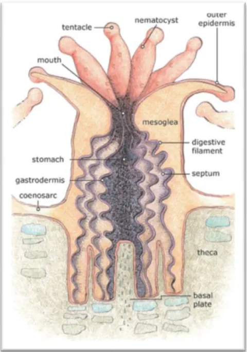
Each polyp has a simple, tube-shaped body, with a circular mouth at the top which also serves as anus. Around the mouth they have numerous tentacles to help capturing food and inside there is a pharynx that connects the mouth to the coelenterons, and has a number of mesenteries poking into it (Spalding, 2004). All exchanges of gases and fluids are happen in coelenterates, because the water enters and leaves the body of the animal by currents caused by tentacles.

They build exoskeletons, and these may be composed by organic matter or calcium carbonate (Glynn & Wellington, 1983). They can also be divided in two types: Hermatypic and Ahermatypic. The first ones can also be called stony corals build reefs and with the help of the zooxanthellae, they convert surplus food to calcium carbonate, forming a hard skeleton. The ahermatypic corals have no zooxanthellae and do not build reefs. These are also known as soft corals and so they are flexible, undulating back and forth in the current, and their skeletons are proteinaceous instead of calcareous as the stony corals (Wells & Hanna, 1992). Both types suffer from environmental influences resulting in limiting the quantity and quality of species.

14

Figure 1 – Basic anatomy of a hard coral polyp. Artwork Credit: NOAA/Gini Kennedy

Corals build colorful and amazing colonies when they find a supportive environment. These great colonies are the most familiar forms of the animals that we know as corals, and their skeletons are the ones that help building and defining coral reefs (Spalding, 2004). These clusters in colonies can reach millions of individuals (polyps), forming a limestone formation, which can have thousands of kilometers. They are home to an ecosystem with an extraordinary biodiversity and productivity.

The polyps have in their tissues a group of plant cells known as zooxanthellae, which are the vegetative state of the dinoflagellate Symbiodinium microadriaticum (Wells et al., 1983).

These zooxanthellae use the sunlight to convert carbon dioxide into carbohydrates, lipids and aminoacids. These products are passed to the host, which in return, produce a nitrogen source (ammonia) and phosphate to algae. Thus, the zooxanthellae takes up the waste of the polyps at the same time that it feeds them, allowing corals to put all their energy into their growth, and consequently into the formation of reefs (Delbeek & Sprung, 1994).

15

1.2

Ecology and Biodiversity

The diversity of coral reefs is comparable with the most rich and diverse terrestrial habitats. These species are considered the base of diversity and despite the reefs occupy a small area of the planet, there are possibly more species per unit area of coral reefs than in any other ecosystem.

Coral reefs are home to a huge variety of organisms, where can be found more than 4000 species of fish. Among them are tropical or reef fish, such as parrotfish, angelfish and butterfly fish, sponges, viruses, crustaceans (including prawns, lobsters and crabs), echinoderms (like starfish, sea urchins and sea cucumbers), sea turtles and sea snakes (Castro & Huber, 2000; Spalding et al., 2001).

Inside of the reefs, like other diverse communities, there is a huge variety of interactions between species. Each one occupies a unique role, or niche, on the reef but because there are so many species, they have to change and adapt. They have to find a space to live and grow, to eat, to avoid being eaten, to hunt, to reproduce and to hide from the hunters (Spalding, 2004).

Some organisms have become masters of camouflage to capture or escape. This co-evolution has also led to a complex two-way interaction between species, including mutualism, where both organisms benefit. One of the most important examples of this partnership is the relationship between the corals and their algae, which has led to the proliferation and success of coral reef builders. Algae use the sunlight and carbon dioxide to produce organic compounds rich in carbon. These in turn are leaked to the polyp and may provide almost all of its nutritional requirements (Allen, 2000).

1.3

Threats to reefs of the Caribbean

The coral reef ecosystems are very sensitive to external impacts that violate its homeostasis, whether natural or human caused. As it is known, almost everywhere there are far fewer corals today than there were even 10-20 years ago. The main causes for this decrease are diseases, sedimentation and nutrient impacts, marine-based pollution, overfishing, direct destruction, coral bleaching and coastal development (Spalding, 2004; Sulu, 2007).

16

1.3.1

Diseases

There are reports of coral diseases since 1970 but it was only in the 1980s and 1990s that some of them had a dramatic impact. In the Caribbean there are over more than 150 species infected, and new diseases continue to be added to the ones already described (Côté & Reynolds, 2006). Infectious diseases can cause population declines or even species extinctions.

Today most of the reefs in the Caribbean have lost 80-100% of their staghorn and elkhorn coral through a disease known as white band disease. Some other coral diseases have been reported and named according to their appearance: white plague, yellow band, black band, dark spots and rapid wasting disease (Spalding, 2004).

Figure 2 – Some of the major coral diseases: 1) white plague; 2) yellow band; 3) white band; 4) black band; 5) red band; 6) white pox; 7) dark spots. Image courtesy by Andy Bruckner, NOAA’s National Marine

Fisheries Service

Coral diseases appear everywhere, but they are more common and more devastating in areas where the corals are already stressed by pollution or sedimentation (Spalding, 2004). Many pathogens are also sensitive to factors as temperature, humidity, and rainfall, and these factors can increase the pathogen development and survival rates, disease transmission and host susceptibility. More research is needed to find if there are points to potential linkages to other stresses on corals as possible instigators of disease (Harvell et al., 2002).

17

1.3.2

Sediments

In the Caribbean, there are increasing levels of sediments in coastal waters. The principal causes of this increase are clearance of forests and movement of agriculture on the steep slopes, leading to soil erosion and these particles are carried by rivers to the sea (Spalding, 2004).

Suspended sediments in the water column can affect coral populations and community structure by suffocating adult corals and enforcing physiological costs by reducing light availability for photosynthesis or increasing the energy needed for sediment removal (Riegl & Branch, 1995). They are able to remove these sediments with their tentacles (sloughing them off with a layer of mucus), but are not able to keep doing it because it uses up energy and resources.

The real understanding of the effects of sedimentation is not easy because the interspecific differences in morphology and sediment rejection ability (Stafford-Smith, 1993); not all the corals have the same ability to use heterotrophic modes of nutrition (Anthony, 2000) and also because sedimentation rates vary with other environmental and biological factors (Babcock & Smith, 2000).

1.3.3

Pollution

Coral-reef ecosystems are highly vulnerable to environmental perturbations in general. This sensitivity has three main factors, and they are: corals have small physiological tolerance for environmental conditions (Johannes, 1975) and any variation of physical-chemical outside these tolerance ranges could be decisive to coral growth and survival (Johannes & Betzer, 1975; Endean, 1976; Pearson, 1981). Another factor is the susceptibility of the interactions of key reef species (like algae-coral competition) to pollutant stresses. The damage of these corals leads to an eventual end of many reef species because these depend on living corals for many reasons like shelter, food and refuge (Johannes, 1975). The third factor that affects corals sensitivity is that the effects of most toxic substances are enhanced in water with high temperatures, which are easily found in coral reef environments (Johannes & Betzer, 1975). These toxic wastes come primarily from detergents, paints, herbicides and pesticides, industrial toxins and oils.

Despite the known toxic wastes, the most widespread form of pollution found on coral reefs comes from simple nutrients like organic matter, nitrates and phosphates. Two of the major sources of these are sewage and agriculture (Spalding, 2004). The potential

18 impacts of sewage effluent on coral-reef communities can be classified in three different categories that represent separate but interacting processes, which are nutrient enrichment, sedimentation and toxicity (Pastorok & Bilyard, 1985).

1.3.4

Overfishing

Humans have gathered and fished coral reef organisms for thousands of years to use it as curios, jewelry and food. More recently, this exploitation has also increased as novel medicinal compounds have been extracted and as reef-related tourism has expanded. According to published work, in the last 30-40 years, increasing populations of humans have been damaging coral reefs at an unprecedented rate (Luchavez & Alcala, 1988; Wilkinson et al., 1993; Munro & Munro, 1994; Grigg & Birkeland, 1997).

Overfishing is one of the major threats to the biological integrity of marine habitats worldwide (Ginsburg, 1994; Dayton et al., 1995; NRC, 1995; Roberts, 1995; Safina, 1995). The removal of grazing species allows algae to overgrow and smother the corals while the removal of small reef fish for commercial sale means that fewer individuals get the chance to grow to reach the reproductive age and replenish the population (Karleskint et al., 2009). Some fishing methods are very destructive, like the careless use of the traps and nets which can smash corals, the use of explosives or bleach to drive fish out of the reef and the use of cyanide (Rubec, 1986; McAllister, 1998, Spalding, 2004) to collect tropical fish for the aquarium trade or fresh fish for local markets. Cyanide is a metabolic poison, and this not only removes great number of fish from the reef but also poisons corals and other invertebrates (Karleskint et al., 2009).

Although everybody knows what to do about overfishing, is incredibly difficult to persuade fishers and politicians to change, because of all the money that is involved. There are still a lot of fish, but not enough to reproduce and restock the reefs, which therefore remain quite unproductive. Well managed, in long-term these same reefs could supply more fish and would also be more attractive to tourists (Spalding, 2004).

19

1.3.5

Coral Bleaching

The phenomenon of coral bleaching affecting extensive reef areas across the Pacific was first described by Glynn in 1984. This process is portrayed as the whitening of corals due to loss of symbiotic algae (zooxanthellae) and/or their pigments and is a global phenomenon that is probably correlated to global climate change and increasing ocean temperatures (Glynn, 1993; Brown, 1997; Hoegh-Guldberg, 1999). Reef-building corals are highly dependent on their zooxanthellae because these provide up to 95% of the corals‟ carbon requirements for growth, reproduction and also maintenance (Muscatine, 1990).

Figure 3 – Partially bleached coral colony (Pocillipora sp.) on a Pacific Reef (A) and close up view of bleached area (B). Photo courtesy by NOAA.

The most important stressor is the variation of sea surface temperature (Glynn, 1984; Cook et al., 1990; Fitt et al., 1993; Brown et al., 1995; Hoegh-Guldberg & Salvat, 1995; Anthony et al., 2008), however things like freshwater flooding (Goreau, 1964; Egana & DiSalvo, 1982), pollution (Jones, 1997a; Jones & Steven, 1997), high turbidity and sedimentation (Meehan & Ostrander, 1997), diseases (Kushmaro et al., 1997; Benin et al., 2000), high levels of ultraviolet light, low light conditions and abnormal salinity (Westmacott et al., 2000) can also cause bleaching on corals.

Most reef corals are very sensitive to environmental stressors that can interfere in the symbiotic relationship with their algae and cause bleaching. Even when corals are pale or white, that doesn‟t mean they are dead, but without its algae they are severely weak and more susceptible to diseases. If conditions do not improve, the coral will inevitably die (Spalding, 2004). Not all coral species are equally affected (Coles & Brown, 2003) and they have different resistance to bleaching (Loya et al., 2001). This difference

20 can be genetically determined or by distribution and environmental variability (McClanahan et al., 2007).

1.4

Porites porites: Biology

Porites is a genus of sceleterian coral which is characterized by a finger-like morphology. The members of this genus have widely spaced calices, a well-developed wall reticulum and are bilaterally symmetrical. Porites porites is a branching species with a more sprawling appearance than the other branching Porites. Branches may be curved, hooked or project downwards and sideways, and are thicker with blunt, enlarged tips. The three branching species are easily confused, and colony shapes overlap. This species has thick branches (˃ 2cm) may be stubby and little developed with enlarged, blunt tips. Developed branches upright or sprawling, often grey, occasionally bright blue. The colonies of this species are common in shallow water near shore where they may form extensive beds (Voss, 2002).

21

1.5

Ocean acidification

Over the past 250 years, the levels of atmospheric carbon dioxide (CO2) increased

by nearly 40%, from preindustrial levels of approximately 280 ppm (parts per million) to nearly 384 ppm in 2007 (Solomon et al., 2007). This rate of increase in atmospheric CO2

is approximately 100x faster than has occurred for millions of years (Siegenthaler et al., 2005) and the current concentration is higher than any level reached in the past 800,000 years (Lüthi et al., 2008). Approximately 25% of the CO2 emitted from all anthropogenic

sources, like human fossil fuel combustion, agriculture, cement production (Houghton, 2001) and deforestation, currently goes to the ocean, where it reacts with water to produce carbonic acid (Hoegh-Guldberg et al., 2007). The CO2 uptake causes pH

alterations, has this already fallen by 0.1 unit, from approximately 8.21 to 8.10 (Royal Society, 2005) compared to pre-industrial times, what means a 30% increase in the H+ concentration and is projected to drop another 0.3-0.4 pH units by the end of this century (Mehrbach et al., 1973; Caldeira & Wickett, 2003; Orr et al., 2005; Loáiciga., 2006; Feely et al., 2009; Anlauf et al., 2011).

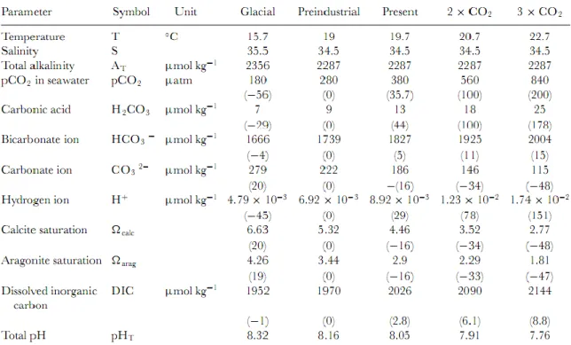
Table 1 – Projected changes in surface ocean carbonate chemistry based on IPCC IS92a

CO2 emission scenario (Guinotte & Fabry, 2008).

Was assumed that PO4 = 0.5 µmol L-1 and Si = 4.8 µmol L-1, and use the carbonic acid dissociation constants of Mehrbach et al. (1973) as refit by Dickson & Millero (1987). pHT is based on seawater scale. Percent change from preindustrial values are in parenthesis. After Feely et al. (2009).

22 When CO2 is absorbed by seawater, a series of chemical reactions happen. An

increase in atmospheric CO2 concentration lowers the pH and the carbonate ion

concentration (CO32-) available (Kleypas & Langdon, 2002). This reduction also leads to a

reduction in calcium carbonate saturation state (Ω), which has big impacts on marine organisms (Guinotte & Fabry, 2008). Table 1 lists the projected changes in surface ocean carbonate chemistry (carbon system parameters and temperature) based on the Intergovernmental Panel on Climate Change (IPCC) IS92a CO2 emission scenario.

One way to predict climate changes is look backward, for example using ice cores. A 2083-meter long ice core with 160,000 years was collected by the Soviet Antarctic Expedition at Vostok, Antarctica (Barnola et al., 1987). There is a close correlation between carbon dioxide in the air and global temperatures over this time. However, there are some difficulties in extrapolating these correlations into the future (Krebs, 1994). The present CO2 levels exceed the levels presented in nature during the last 160,000 years so

is not known if it‟s correct to extrapolate with the same relationship found in the past. Another problem is the velocity at which CO2 levels are changing. Year to year they are

changing. Lessons learned about the relationship between CO2 and climate in the past will

have to be applied with caution in predicting the future climate because the rate of change of climate forcing is very different today.

The rate of this change is really concerning biologically as well, since many marine organisms, particularly the calcifying ones, may not be able to adapt quickly enough to survive to these changes. Some of the most abundant life forms that will be affected are plankton. These are very important because they form the base of the marine food chain and are a major food source for fish and marine mammals (World Bank, 2010). Acidification may decrease reef growth by reducing calcification rates but also reproduction and recruitment (NRC, 2010).

Coral reefs are among the marine ecosystems most vulnerable to the changing climate and atmospheric composition and are threatened by a combination of direct human impacts and global climate change. Coral reefs are already being pushed to their thermal limits by recent temperature increases (World Bank, 2009).

Diverse studies identify the ocean acidification as a threat to marine biota for different factors such as: the calcification rates of shell-forming organisms in response of supersaturation (Smith & Buddemeier, 1992; Kleypas et al., 1999); aragonite, a mineral also very important to organisms that calcify, may become undersaturated in the surface ocean in the early 21st century (Feely & Chen, 1982; Feely et al., 1988; Orr et al., 2005); and the effects of the decreasing of pH go far beyond limiting calcification.

It is already known that calcification of corals and coral communities is controlled by saturation of seawater with respect to aragonite (Gattuso et al., 1999; Langdon et al.

23 2000; Leclerq et al., 2000; Leclerq et al., 2002). Several papers have tried to predict the future response of calcification by coral communities, using the experimental evidence of previous works, to elevated pCO2 and its biogeochemical significance. Is consensual that

calcification rate will decrease by 14-30% by 2100 (Gattuso et al., 1999; Kleypas et al., 1999).

One of the most obvious and well documented effects of ocean acidification is, as it was said before, the decrease of calcification rates, affecting skeletal growth. There are records that on the Great Barrier Reef, massive corals showed a decrease in calcification rates by about 14% between 1990 and 2005 (De‟ath et al., 2009). In stony corals, most studies indicate a 10-60% reduction in calcification rate for a doubling of preindustrial atmospheric CO2 concentration. The differences between studies may be due to different

species or experimental setups (Doney et al., 2009; Kleypas et al., 2006; Langdon & Atkinson, 2005).

Growth of the reef structures also rely on the successful recruitment of reef organisms, which is determined by gamete production, fertilization rates, larval development and settlement, and post-settlement growth. In general, there are a few data on any of these aspects for reef-building species, making extrapolation to ecosystem effects difficult (Jokiel et al., 2008; Albright et al., 2008).

1.5.1

Ocean carbonate system

The carbon system is one of the most important components of oceanography, primarily because it acts as a governor for the carbon cycle and also because it controls the acidity of seawater. This system also plays a very important role controlling the pressure of carbon dioxide in the atmosphere, helping to regulate the temperature of the planet (Emerson & Edges, 2008).

Seawater carbonate chemistry is a series of chemical equilibria, led mainly by DIC (Dissolved Inorganic Carbon) and TA (Total Alkalinity) (Kleypas et al., 2006). The surface water CO2 to atmospheric levels is equilibrated by exchanges between air and sea in a

timescale of approximately one year. When CO2 dissolves in seawater, it reacts with the

water and form carbonic acid (H2CO3), which will lose hydrogen ions to form bicarbonate

(HCO3-) and carbonate (CO32-) (Doney et al., 2009).The basic equations describing this

24 CO2 (g) CO2 (aq)

CO2 (aq) + H2O H2CO3

H2CO3 H+ + HCO3

-HCO3- H+ + CO3

2-Processes that increase DIC shift the equilibrium in a way to lower the pH and lower CO32- concentration; on the other hand, processes that increase TA shift the equilibrium in

a way to increase the pH and CO32- concentration. Calcification and dissolution affect both

DIC and TA, while respiration and photosynthesis primarily affect DIC (Kleypas et al., 2006).

1.5.2

Calcification and Dissolution response from Hermatypic Corals

The reef-building corals, zooxanthellate, are a very important group with the capacity to produce massive quantities of calcium carbonate (Stanley & Hardie, 1998). A lot of experiments were performed to test the response of calcification rate to decreases in aragonite saturation state, and some evidences indicate that the calcification rate of tropical reef-building corals will be reduced by 20-60% at double preindustrial CO2

concentrations (Gattuso et al., 1998; Kleypas et al., 1999; Langdon et al., 2000; Kleypas & Langdon, 2002; Langdon et al., 2003; Reynaud et al., 2003; Langdon & Atkinson, 2005; Royal Society, 2005; Kleypas et al., 2006).

Calcification rates vary under different environmental conditions and the most important are light, temperature and nutrients (Doney et al., 2009). Light increases the primary productivity of coral reefs and provides the precipitation of CaCO3 in

zooxanthellate corals (Falkowski et al., 1990) and coralline algae (Johansen, 1981). Marubini et al., 2001 found out that calcification increases with increasing light up to a limit and then saturates. Temperature also affects the calcification rate, as proved in a lot of literature. Most of species calcify faster with an increase in temperature until an optimal temperature at or 1º - 2ºC below the normal peak summer temperature, after this point calcification rates starts to decline (Clausen & Roth, 1975; Jokiel & Coles, 1977). Nutrient concentration was also found to affect coral calcification in laboratory studies. The

25 principal studied nutrients were nitrate and ammonium. Enrichment of nitrate to levels of 5-20 µM resulted in increased zooxanthellae density and photosynthesis, and so decreased calcification rate (Marubini & Davies, 1996; Marubini & Thake, 1999). Also an increase in the ammonium concentration produces similar results (Ferrier-Pages et al., 2000; Hoegh-Guldberg & Smith, 1989; Stambler et al., 1991).

1.6

Objectives

This study aims to investigate the effects of global environmental changes on the physiology of scleractinian corals in order to reach better predicting capabilities on their response to future changes. The effects of increases of CO2 were investigated using

concentrations of 390 ppm (actual concentration found in seawater), 1350 and 6000 ppm. The experimental coral chosen for this study was the ecological significant species Porites porites. To achieve that, specific objectives were drawn:

1. To evaluate the effects of high CO2 in corals growth using:

a. Buoyant Weight; b. Linear Extension;

2. To determine and analyze the zooxanthellar density for corals in high CO2

levels and in control;

26

2.

Material and Methods

2.1 Preparation of corals

Branches of Porites porites were brought from the Smithsonian laboratory in Fort Pierce, FL to RSMAS (Rosenstiel School of Marine & Atmospheric Science) in January 2011. There they were placed in a tank, 380 L, inside the Experimental Corals and Climate Change Facility and kept at a temperature of 27ºC and a salinity at 36.5. In April 2011, tips were removed from the branches and their cut faces were ground flat. They were then prepared into coral „nubbins‟ as described in Davies (1995) and glued with All Game Epoxy II-Part putty on PVC plastic tiles (35 x 37 mm). After the „nubbins‟ were done, they were placed in a smaller tank with 262 L of seawater, which was called control, since the CO2 level was 390 ppm. They were kept there for one week so they could

recover and then were switch to the different CO2 levels.

2.2 Experimental setup

An experiment was performed to evaluate the effect of different CO2 levels on

growth and calcification of Porites porites. The experiment was done in the Experimental Corals and Climate Change Facility of RSMAS and lasted for eight weeks, from April 21st to June 15th.

This facility is composed by twelve fiberglass tanks measuring 0.6 x 0.5 m filled to a depth of 0.22 m. The tanks are inside a shadehouse with a polypropylene clear plastic roof that admits natural sunlight but at the same time, protects the equipment from the elements. The nominal amount of sunlight reaching the organisms varies seasonally but is typically 6-8 mol photons m-2 d-1. The tanks are supplied by high quality low nutrient concentration natural seawater from the nearby Bear Cut entrance to Biscayne Bay. The salinity also varies seasonally but usually is between 33 and 38. The water from the Bear Cut is pumped into a 50,000 gallon settling tank and then through a series of filters that are intended to remove particulates down to a size of 10 µm. This seawater flows to each of the experimental tanks at a rate of approximately 150-200 ml min-1. These experimental tanks contain 60 L of seawater and are associated with a 200 L sump tank. The seawater from the sump tank into the experimental tank is continuously circulated by a magnetically coupled 500 GPH pump which is in the sump tank. This seawater pumped sprays out

27 through some holes made in a length of ½” PVC pipe that is in the bottom of the experimental tank, generating lots of turbulence within the tank in proximity to the corals. The seawater in the experimental tanks is exchanged with the seawater in the sump approximately every 10 minutes and through a standpipe.

Each sump tank is fitted with a 1500-watt tungsten heater and heat exchanger coil made of 1” polypropylene irrigation tubing. A solenoid valve is used to block or permit the circulation of chilled freshwater (20ºC) through the heat exchange coil. There is also an Omega CN7500 digital temperature controller that is able to hold the average daily temperature to ±0.1ºC.

The CO level in the experimental tanks is controlled by bubbling the seawater in the sump tanks with a CO2-enriched air mixture. An air compressor delivers air with a pCO2 of

390 ppm to a centrifugal drier. The dried air at a pressure of 14 psi is connected to several Sierra Instruments 810C Mass Flow Controllers (MFC). These deliver a steady stream of dried air at a precisely controlled rate that is adjusted to 6-14 L per minute. A second set of MFCs are connected to a cylinder of instrument grade CO2 gas. These are adjusted to

a supply stream of CO2 gas at flow rates ranging from 5-100 ml per minute. The outputs of

air and CO2 MFCs are connected in pairs to gas mixing tubes. Adjusting the setting n the

two MFCs can precisely control the pCO2 of the mixture. The flow rate of gas mix going to

each tank is monitored using a rotameter, and by determination a flow rate of 3-5 L per minute was found to be adequate for controlling the pCO2 in the experimental tanks. From

the rotameter the gas mix goes to a venturi injector. This produces a strong stream of bubbles that promotes the exchange of CO2 in the gas mix with the seawater in the sump

tanks. To achieve a desired CO2 level, the pCO2 of the gas mix needs to be adjusted

empirically to compensate for the gas exchange and the rate that CO2 is added and

removed from the system by the flow of Bear Cut seawater. An equilibrator/IRGA system monitors the pCO2 of the seawater actually achieved on the tanks and an Onset Computer

HOBO data logger acquires the temperature of each of the experimental tanks, the tank pCO2 and the incoming photosynthetically available irradiance every 5 minutes.

In this experiment, three different levels of CO2 were used to test the effects of this

28

Figure 5 – Tanks inside of the Experimental Corals and Climate Change Facility at RSMAS, where corals were placed. Photo by the author

The corals were feed every Thursday with a special recipe composed by 134 ml of phytoplankton, 0.6 g of oystereggs, 0.6 g of larval food supplement 100-150 microns, 0.6 g of larval food supplement 250-450 microns and 50 ml of seawater. Before the feeding the water flow was turned off and the temperature was take down to 24.8º C.

2.3 Measurements

2.3.1 Buoyant Weight

Coral growth was measured by buoyant weighing (Davies, 1989) once every 2 weeks until May 15th and then weekly. An electronic balance was used, reading to 0.1 mg. The balance was mounted on a wooden box whose interior formed the weighing chamber. The front was fitted with a transparent door, which could be closed to exclude air movements during weighing. After all setup, the coral was handled by the tile to minimize damage to the tissues and hold inside of a container filled with seawater maintained at the same temperature and salinity so the density wouldn‟t change.

Final skeletal growth rates were obtained by linear regression of weight against time over the last 7 weeks of the experiment only, because the first measurement was relative

29 to the week they were under control. At the end of the experiment the surface area of live tissue of each colony was determined and the growth rate was normalized to the cm2 of live tissue.

Buoyant weight is the weight of the coral in water, so it was necessary to calculate the weight of coral in air. The equation used was the one that is below (Eq. 1) and has been explained in more detail by Jokiel et al., 1978.

Eq. 1 – Equation to calculate the weight of object in air (Davies 1989)

where wt in water = weight (g) of the object in water, Dwater = density (g/cm3) of the

seawater, Dobject = density (g/cm3) of the object being weighed. For the density of the

object was used the value of 2.822 g/cm3, which was direct determined for Porites porites by Edmund & Davies, 1986. The Dwater was accurately determined from Eq. 2 by weighing

an inert reference object of known air weight and density in the seawater. The object used was glass and its density was calculated from Eq. 3.

30

Eq. 3 – Equation to calculate the Density of object (Davies 1989)

The temperature and the salinity of the seawater were always controlled during the buoyant weighing and kept at 27ºC and 35 respectively, so the density didn‟t change.

2.3.2 Linear Extension

Another way to measure the coral growth was through linear extension using a micrometer. The height of the corals was measured almost every week during all experiment.

The linear extension was measured using an optical micrometer, capable of measuring linear extension rates to a precision of 0.5 µm. During each measurement period, the corals were placed into bins filled with seawater and taken to the lab. There they were briefly removed from the bin, fitted onto the stage of the micrometer, and advanced through the path of the optical micrometer. Each measurement was conducted in no longer than 4 minutes, thereby minimizing the time they were out of water.

The average growth rate was obtained from regression equations of maximum point (maximum height) against time over 5 weeks of the experiment only, because like in the buoyant weight one of the weeks the corals were still in controls and the other week that there‟s no data, was because the Micrometer wasn‟t not on the lab.

31

Figure 6 – Micrometer used to the Linear Extension (L.E.). Photo by the author

Figure 7 – Coral being measured by L.E. Photo by the author

Figure 8 – Example of a graph for growth rate by Linear Extension

-25 -20 -15 -10 -5 0 5 10 0 10 20 30 40 H e ig h t (m m ) Distance (mm) April-20 May-10 May-20 May-28 June-6 June-13

32

2.3.3 Chlorophyll a concentration

After the end of the experiment, all the corals were brought to the Baker lab in RSMAS where they were blasted, that is, the tissues were removed from the skeletons with a jet of filtered seawater using a WaterPikTM (Johannes & Wiebe, 1970). The volume of the blastate was made up to 50 ml using filtered seawater. Subsamples of the blastate were taken for analysis of zooxanthellar densities and chl a concentration.

For the chlorophyll a concentration, 1 ml of the blastate was placed in a glass tube, 9 ml of 90% acetone was added with a graduated cylinder and the sample was put in an -80ºC freezer for about 30 hours. After this time, the sample was brought to room temperature and vortexed to remove filter fibres from suspension. 0.5 ml of the sample was removed to a tube and 3 ml of 90% acetone was added (Nakamura et al. 2003). The sample was put into the Fluorometer TD-700 Turner Designs, and the first read of absorbance was taken. After this, 1 drop of 10% HCl was added to acidification and the second read taken.

The follow equation was used to calculate the concentration of Chlorophyll a

Chla = (1x10

) * D * (K * T) * (Fo-Fa)

where Chla is the amount of the pigment in the coral tissue sample in µg, the factor

10-3 converts from liters to milliliters, D is the overall dilution (50:1)*(10:1)*(7:1) or 3500, K is the calibration constant (K = 0.0000892904 µg/mL), T is the maximum ratio of chlorophyll a fluorescence before and after adding acid (T = 1.885908293), Fo is the first fluorescence reading, Fa is the second fluorescence reading after adding the HCl. Finally the pigment results were divided by surface area of the coral to obtain the µg Chla per cm2 of coral tissue.

2.3.4 Zooxanthellar density

1.5 ml of the 50 ml blastate solution was put into Eppendorf tubes and 30 ml of Lugols added (i.e. 1.5:31.5 dillution). The tubes were stored out of the light. The samples

33 were then vortexed and a portion pulled up into a Pasteur pipette. A haemocytometer was positioned on edge of microscope platform with coverslip, and filled by capillary action.

A counter was used to count all cells falling within or on the lines defining the 9 squares of the haemocytometer. The counts were recorded in a table under the sample number and some repeats were done loading the haemocytometer at least 3-5 times. The volume of liquid counted (9x10-4 ml), the volume of the blastate counted (1.5 ml), the dilution of the blastate (1.5:31.5) and the surface area of the coral were used to calculate the density of zooxanthellae cells per cm2.

The formula used to calculate the density of zooxanthellae was the following one:

Z = (N/9x10-4)*D/SA

Where Z is the zooxanthellae density in cell per cm2 of coral tissue, N is the average number of zooxanthellae counted in the haemocytometer slide, 9x10-4 ml is the volume of Lugol solution counted, D is the overall dilution factor (50:1)*(31.5:1.5) and SA is the surface area of the coral.

2.3.5 Surface area determination

Measurements of coral growth rate were made and determinations of zooxanthellae densities and chlorophyll concentrations. However, the results were taken from different sizes of coral “nubbins”, which required a method of „normalizing‟ the amount of coral in the analyses. The most common method is to use the surface area of the colonies to account for the different amount of biomass in each measurement.

The method used in this specie to measure the surface area was the Aluminum foil (Marsh, 1970) since it works well for “boulder” corals like Porites porites. To determinate it, after removal of tissue from the coral, an Aluminium foil was layed over the coral surface, using scissors to trim the foil to cover the entire blasted area. Then the foil was stretched and a picture was taken. In the program “Image J” the image was treated and the surface was calculated.

34

2.4 Statistical analyses

The effect of high levels of CO2 on coral growth rate was tested for each experiment

by separate One-way ANOVAs. Calcification rate by buoyant weight, chlorophyll a concentration and zooxanthellae density per nubbin were positively correlated to final surface area, so this was used to normalize the data. Statistical differences were considered for P ˂ 0.001.

All the statistical analysis were performed using the “data analysis package” from Microsoft Office, Excel.

35

3.

Results

3.1 Chemical conditions

The chemical conditions for the treatment are summarized in Table 2. The temperature was maintained at 27.1 ± 0.5ºC and the salinity at 36.4 ± 0.2. The Total Alkalinity (TA) ranged from 2147 ± 115 for the higher level of CO2 to 2282 ± 79 µmol kg-1

for the lower level. The values of pH and Ωaragonite were between 7.1 ± 0.1 and 0.6 ± 0.1 for

the lower level respectively, and 8.1 ± 0.04 and 3.9 ± 0.4 for the higher level.

Table 2 – Physical and chemical conditions during the laboratory experiment 1. Data

given as means ± SD Salinity Temp. (ºC) CO2 (ppm) TA (µmol/kg) pH Ωaragonite April Low 36.1 ± 0.64 26.8 ± 0.62 329.4 ± 46.94 2068.8 ± 61.82 8.09 ± 0.08 3.58 ± 0.40 Medium 36.5 ± 0.33 27.0 ± 0.73 1325.5 ± 134.24 2182.4 ± 43.30 7.57 ± 0.03 1.37 ± 0.08 High 36.5 ± 0.26 27.1 ± 0.69 4316.2 ± 671.63 2364.3 ± 96.40 7.72 ± 0.14 0.57 ± 0.06 May Low 35.7 ± 0.91 27.1 ± 0.49 263.3 ± 7.70 2137.2 ± 59.07 8.15 ± 0.02 3.96 ± 0.18 Medium 36.8 ± 0.35 27.1 ± 0.30 1477.0 ± 156.84 2115.5 ± 45.30 7.52 ± 0.06 1.22 ± 0.15 High 36.6 ±0.45 27.2 ± 0.39 4155.8 ± 224.42 2254.2 ± 25.41 7.12 ± 0.02 0.54 ± 0.02 June Low 35.6 ± 0.82 27.1 ± 0.06 295.1 ± 17.33 2333.5 ± 148.21 8.15 ± 0.002 4.42 ± 0.31 Medium 36.8 ± 0.33 27.1 ± 0.08 2274.1 ± 1202.61 2242.7 ± 19.90 7.39 ± 0.22 1.06 ± 0.43 High 36.9 ± 0.26 27.3 ± 0.11 3775.3 ± 905.01 2248.9 ± 63.48 7.16 ± 0.11 0.62 ± 0.16

36

3.2 Growth rates

The effects of different levels of CO2 on growth of corals were determined by

buoyant weight and linear extension. The data related to that effect is presented in Tables 3 and 4, for buoyant weight and linear extension respectively.

3.2.1 Buoyant Weight (B.W.)

Table 3 – Mean initial weight, surface area and growth rate for Porites porites calculated

by buoyant weight. Data given as means ± SE

Treatments CO2 level (ppm) Ωaragonite n Initial weight (g) Surface area (cm2) Growth rate (mg d-1 cm-2) Low 390 3.6 6 14.7 ± 0.9 27.2 ± 3.6 17.7 ± 0.7 Medium 1350 1.3 5 15.9 ± 0.9 27.7 ± 3.5 11.2 ± 0.7 High 6000 0.4 5 15.1 ± 0.8 22.0 ± 2.1 4.0 ±1.7

In the Buoyant weight, the average initial weight of nubbins was 15.2 ± 0.5 g and the surface area was 25.9 ± 1.9 cm2. A decrease in the growth rate was observed for the higher values of CO2 in the end of the experiment. The values recorded ranged from 17.7

± 0.7 for the low level treatment (390 ppm) to 4.0 ± 1.7 mg d-1 cm-2 for the high level treatment (6000 ppm). In a 95% confidence, really small error bars were presented, which mean that the results are really reliable (Figure 9).

37

Figure 9 – Growth rate by buoyant weight for Porites porites in the end of experiment. Error bars are 95% confidence

Another very important variable is the aragonite saturation state (Ω). In the 390 ppm treatment, Ω was kept at 3.6, in the 1350 ppm kept at 1.3 and finally, in the 6000 ppm maintained at 0.4. The relation between the growth rate and the saturation state it‟s almost linear, corresponding the lowest growth rate to the lower Ω and the highest growth rate to the highest Ω (Figure 10).

The growth rate by the technique of buoyant weighing for the control and the two levels of CO2 was statistically different (P˂0.001), so big differences were found within or

between experiments.

Figure 10 – Scatterplot of average growth rate by Buoyant Weight per tank (g d-1

) to Aragonite saturation state (Ω) 0 0,05 0,1 0,15 0,2 0,25 0,3 0,35 390 1600 6000 g o f w ei ght cha nge in 8 w e e ks CO2 Levels (ppm) 390 1600 6000 0,004 0,0112 0,0177 0 0,002 0,004 0,006 0,008 0,01 0,012 0,014 0,016 0,018 0,02 0 1 2 3 4 Gr o wt h r ate (g d -1)

Aragonite saturation state

6000 1350 390

38

3.2.2 Linear Extension (L.E.)

Table 4 – Mean initial height and growth rate for Porites porites calculated through linear

extension. Data given as means ± SE

Treatments CO2 level (ppm) n Initial height (mm) Growth rate (µm/d) Low 390 6 16 ± 2 99 ± 7 Medium 1350 5 17 ± 2 45 ± 8 High 6000 5 19 ± 1 16 ± 3

Regarding the linear extension, the results were really similar to the ones obtained from buoyant weight. A decrease in the growth rate was observed for the higher levels of CO2. For the Low level treatment the growth rate was 99 ± 7 and for the High level this

was 16 ± 3 µm d-1.

Statistically, the growth rate calculated by linear extension for the control and the two levels of CO2 was also very different (P˂0.001), which means that big differences

were found within or between experiments.

Figure 11 - Scatterplot of average growth rate by Linear Extension per tank (mm d-1) to Aragonite saturation state (Ω) 0,01556 0,04486 0,09852 0 0,02 0,04 0,06 0,08 0,1 0,12 0 1 2 3 4 Gr o wt h r ate (m m d -1)

Aragonite Saturation State (Ω)

6000 1350 390

39

3.2.3 Combined data

To a better understanding of the effects of CO2 on growth rate of the corals, the two

different methods were analyzed together.

Comparing both methods of growth (Figure 12) was understandable that the growth rate for the linear extension was higher than the one for the buoyant weight. However, for all the corals, the growth rate by buoyant weight was much more linear and constant.

Figure 12 – Growth rates through the two methods: Linear extension (blue) and Buoyant weight (red) for the different levels of CO2

3.3 Chlorophyll a concentrations and Zooxanthellae density

High levels of CO2 showed a decline both in numbers of zooxanthellae and

chlorophyll concentration per unit surface area. The Chlorophyll concentration in 390 ppm ranged from 4.7 to 9.1 µg cm-2 (Table 5), whereas those exposed to 6000 ppm ranged from 1.0 to 2.5 µg cm-2. Zooxanthellae densities for the 390 ppm were between 3,500,000 and 3,800,000 cells cm-2 and for the 6000 ppm between 310,000 and 1,100,000 cells cm

-2_. y = 25,35x + 8,13 R² = 0,87 y = 2,52x + 2,54 R² = 0,81 -2 0 2 4 6 8 10 12 14 0 20 40 60 80 100 120 140 0 1 2 3 4 Gr o wt h R ate

Aragonite Saturation State (Ω)

Linear Extension (um/d) Buoyant Weight (mg/d/cm2)

40

Table 5 – Chlorophyll a concentration and number of zooxanthellae per area. Means ± SE CO2 Level (ppm) # Coral Chlorophyll a (µg/cm2) Average Zooxanthellae cells/cm2 Average 390 70 4.7 6.7 ± 0.6 3,700,000 3.6 x 106 ± 4.5 x 104 73 6.5 3,500,000 74 5.9 3,600,000 79 7.5 3,500,000 85 9.1 3,800,000 88 6.7 3,600,000 1350 72 2.1 3.9 ± 0.5 2,600,000 3.2 x 106 ± 1.5 x 105 75 5.0 3,600,000 76 5.0 3,300,000 80 4.1 3,300,000 86 3.6 3,200,000 6000 77 2.5 2.0 ± 0.3 960,000 9.1 x 105 ± 1.5 x 105 78 1.0 310,000 83 2.5 1,100,000 84 2.4 1,000,000 87 1.4 1,100,000

For a better understanding of the chlorophyll concentration and number of zooxanthellae in corals during the experiment, the average per surface area was calculated for the three different levels of CO2 and represented by the Figure 13 and 14,

respectively.

A One-way ANOVA found that carbon dioxide concentration has a highly significant effect on chlorophyll a concentration and zooxanthellae density, being P˂0.001.

Figure 13 – Average concentration of Chlorophyll a per unit of area (cm2

) for the different levels of CO2. Error bars are 95% confidence.

0 1 2 3 4 5 6 7 8 9 390 1350 6000 Ch lo ro p h yl l a c o n ce tr ation s (µ g c m -2) CO2 levels (ppm) 390 1350 6000

41

Figure 14 – Concentration of Chlorophyll a per unit of area (cm2

) for the different levels of CO2 and respectively power regression.

Figure 15 – Number of zooxanthellae/cm2

for the different levels of CO2. Error bars are 95% confidence.

0 500000 1000000 1500000 2000000 2500000 3000000 3500000 4000000 390 1350 6000 Zo o xan th e llae c e lls cm -2 CO2 Levels (ppm) 390 1350 6000

y = 101,02x

R² = 0,9993

42

Figure 16 – Number of zooxanthellae/cm2

for the different levels of CO2 and respectively linear regression

The chlorophyll concentrations in zooxanthellae, presented a different result from the other analysis. A higher value of µg chlorophyll per zooxanthella was observed for the highest CO2 level (6000 ppm) instead for the control (Figure 17). The values ranged from

1.2 x 10-6 for the medium level (1350 ppm) to 2.3 x 10-6 for the highest level of CO2.

Figure 17 – Chlorophyll a concentrations per number of zooxanthellae for each treatment. Error bars are 95% confidence. 0 0,0000005 0,000001 0,0000015 0,000002 0,0000025 0,000003 0,0000035 390 1350 6000 µ g Ch lo ro p h yl l a /Z o o xan th e llae CO2 Levels (ppm) 390 1350 6000 y = -473,64x + 4E+06 R² = 0,9986 0,00E+00 5,00E+05 1,00E+06 1,50E+06 2,00E+06 2,50E+06 3,00E+06 3,50E+06 4,00E+06 0 1000 2000 3000 4000 5000 6000 7000 Zo o x cm -2 CO₂ (ppm)

43

3.4 Light data

Keeping the amount of light received as close as possible with the natural conditions on ocean is one of the things to have in attention in an experiment. Light has a central role in primary productivity of coral reefs and provides the precipitation of CaCO3 skeletons in

hermatypic corals (Falkowski et al., 1990). Figure 18 represents the values obtained for everyday during the experiment, which ranged from 6.0 to 15.1 mol photons m-2 d-1.

Figure 18 – Total of light (mol photons/m2

)emitted per day

0 2 4 6 8 10 12 14 16 04.21 04.23 04.25 04.27 04.29 05.01 05.03 05.05 05.07 05.09 05.11 05.13 05.15 05.17 .1905 05.21 05.23 05.25 05.27 05.29 05.31 06.02 06.04 06.06 06.08 06.10 06.12 06.14 To tal lig h t m o l p h o to n s m -2 p e r d ay Dates

44

3.5 Bleaching

After 7 weeks of exposure to high levels of CO2 (6000 ppm) all the corals that were

in this treatment became white (loss of pigmentation), starting to bleach, as shown in the picture below (Figure 19). The corals that were in the other treatments didn‟t show any signal of bleaching.

Figure 19 – The left coral belonged to the control tank (390 ppm), while all the other belonged to the high level of CO2 (6000). A big difference in color can be seen. Photo by the author.

45

4.

Discussion

4.1 Growth rates

In this experiment, the effect of increased CO2 concentration in seawater was tested

for the species Porites porites. The results showed that this increase causes a decrease in the growth rate of this hermatypic coral skeleton, which means that calcification in this species depend not only but also on dioxide carbon concentration.

Three different levels of CO2 were used, being one the control (390 ppm) and

another two levels, 1350 and 6000 ppm. These two values are higher than the ones predicted to the next century, but they were chosen out of curiosity about what may happen in coming centuries if human society does not bring CO2 levels under control. The

390 ppm corresponded to a saturation state of 3.6, the 1350 ppm to a Ω = 1.3 and finally, the 6000 ppm to a Ω = 0.4.

Growth rates in this experiment are similar to previous estimates for nubbins of Porites compressa and Porites porites grown in the laboratory (Marubini & Davies, 1996, Marubini & Atkinson, 1999, Marubini & Thake, 1999, Marubini et al., 2001, Gattuso et al., 1999) and in the field (Edmunds & Davies, 1986, Edmunds & Davies, 1989). Since weight gain is a function of colony size and this is artificially determined when nubbins are cut off the mother colony, it‟s important to control the size for when measuring growth rate (Marubini et al., 2001). There are many ways to estimate colony size, being the more important, surface area (Barnes & Taylor, 1973, Rinkevich & Loya, 1984), skeletal weight, protein, chlorophyll and tissue content (Marubini et al., 2001). In this study the interest was the growth response to increased levels of carbon dioxide and decreased saturation state, as chlorophyll a concentration and zooxanthellae density. For this reason, surface area was used, since it is linearly correlated to growth rate and controls for colony size.

That is a lot of literature that provides evidence of detrimental effects on corals of increased pCO2 alone or in combination with other factors (Gattuso et al., 1999, Ohde &

van Woesik, 1999, Leclerq et al., 2000, 2002, Langdon et al., 2003, Marubini et al., 2003, Reynaud et al., 2003, Renegar & Riegl, 2005). However none of these studies was done with the species Porites porites neither with such high values of CO2 and low values of

saturation state.

For the buoyant weight, the values recorded ranged from 17.7 ± 0.7 for the control to 4.0 ± 1.7 mg d-1 _cm-2 _{for the high level treatment, which shows a really big decrease in the}

growth rate. Results obtained for the species Porites compressa by Marubini et al., 2001, showed that nubbins grown in conditions of the Last Glacial Maximum (target values: Ω =