i
Unsupervised feature extraction with Autoencoder
for the representation of Parkinson’s disease patients
Veronica Kazak
Dissertation presented as partial requirement for obtaining the
Master’s degree in Information Management
MGI
Mestrado em Gestão de Informação
Master Program in Information Managementii
Instituto Superior de Estatística e Gestão de Informação Universidade Nova de Lisboa
UNSUPERVISED FEATURE EXTRACTION WITH AUTOENCODER
FOR THE REPRESENTATION OF PARKINSON'S DISEASE PATIENTS
by
Veronica Kazak
Proposal for Dissertation presented as partial requirement for obtaining the Master’s degree in Information Management, with a specialization in Knowledge Management and Business
Intelligence
Advisor: Professor Roberto Henriques, PhD Co-Advisor: Professor Mauro Castelli, PhD
iii
Abstract
Data representation is one of the fundamental concepts in machine learning. An appropriate representation is found by discovering a structure and automatic detection of patterns in data. In many domains, representation or feature learning is a critical step in improving the performance of machine learning algorithms due to the multidimensionality of data that feeds the model. Some tasks may have different perspectives and approaches depending on how data is represented. In recent years, deep artificial neural networks have provided better solutions to several pattern recognition problems and classification tasks. Deep architectures have also shown their effectiveness in capturing latent features for data representation.
In this document, autoencoders will be examined to obtain the representation of Parkinson's disease patients and compared with conventional representation learning algorithms. The results will show whether the proposed method of feature selection leads to the desired accuracy for predicting the severity of Parkinson’s disease.
Keywords:
Autoencoder, Representation Learning, Feature Extraction, Unsupervised Learning, Deep Learning.
iv
Developing this master's thesis initially seemed extremely challenging due to requirements for conducting research in the field of deep learning but it has been made possible by the support of some people to whom I would like to express my sincere gratitude.
First and foremost, I would like to thank my two advisors Prof. Dr. Roberto Henriques and Prof. Dr. Mauro Castelli. You both provided me with a perfect balance of guidance and freedom. Prof. Dr. Roberto Henriques became my guide in the world of data science – first, planting the seed of curiosity in the area and then, encouraging my research. Thank you for helping me to have carried out research and for all your valuable advice in developing the document.
Prof. Dr. Mauro Castelli played a key role in determining the area of research suggesting the source of data on Parkinson's disease patients. Thank you for your availability and support as well as for solving doubts in training neural networks.
I would also like to thank Prof. Dr. Pedro Cabral for teaching me the standards and guidelines for scientific research and writing. Thanks to Professor, I managed to organize the process as from the earliest stage and comply with deadlines.
I would also like to express my special thanks to Eran Lottem, the neuroscientist from Champalimaud Foundation who inspired me for studying deep learning. Being a brain scientist, he triggered my interest in artificial neural networks that simulate a real brain. Our talks about brain activity strengthened further my decision to do this research.
I also want to thank my friends and fellow colleagues for your moral support and contributing to keep my mental energy.
Last but not least, truly heartfelt and great thanks to my family and my loved ones Laurent Filipe Iarincovschi, Ivan Iarincovschi and Svetlana Kalinina for your blessings, for the amazing support and always being on my side giving the strength to continue and conclude this work.
Sincere thanks to all, Veronica Kazak.
v
Contents
CHAPTER 1 INTRODUCTION ... 1 1.1 MOTIVATION ... 1 1.2 BACKGROUND ... 1 1.2.1 Theoretical framework ... 11.2.2 Autoencoders in medical data research ... 3
1.3 STUDY RELEVANCE ... 4
1.4 OBJECTIVES ... 5
CHAPTER 2 NEURAL NETWORKS: DEFINITIONS AND BASICS ... 6
2.1 INTRODUCTION TO ARTIFICIAL NEURAL NETWORKS ... 6
2.1.1 Single perceptron ... 6
2.1.2 Multilayer perceptron ... 7
2.1.3 Activation functions ... 9
2.1.3.1 Sigmoid activation function ... 9
2.1.3.2 Hyperbolic tangent activation function ... 10
2.1.3.3 Rectified Linear Unit (ReLU) activation function ... 10
2.1.3.4 Softmax activation function ... 11
2.2 TRAINING ARTIFICIAL NEURAL NETWORKS ... 12
2.2.1 Backpropagation ... 12
CHAPTER 3 AUTOENCODER FRAMEWORK ... 16
3.1 OVERVIEW ... 16 3.2 AUTOENCODER ALGORITHM ... 17 3.3 PARAMETRIZATION OF AUTOENCODER... 17 3.3.1 Code size ... 17 3.3.1.1 Undercomplete Autoencoders ... 18 3.3.1.2 Overcomplete Autoencoders ... 18 3.3.2 Number of layers ... 18
3.3.2.1 Restricted Boltzmann machine ... 18
3.3.2.2 Deep belief network ... 20
3.3.2.3 Stacked autoencoder ... 20
3.3.3 Loss function ... 21
3.3.3.1 Mean squared error loss function ... 22
3.3.3.2 Cross entropy loss function ... 22
3.3.4 Optimizer ... 22
3.3.5 Regularization ... 23
vi 3.4 OTHER AUTOENCODERS ... 28 3.4.1 Variational Autoencoder ... 28 3.4.2 Convolutional autoencoder ... 29 3.4.3 Sequence-to-sequence autoencoder ... 31 3.5 AUTOENCODERS SUMMARIZED ... 32 CHAPTER 4 METHODOLOGY ... 34
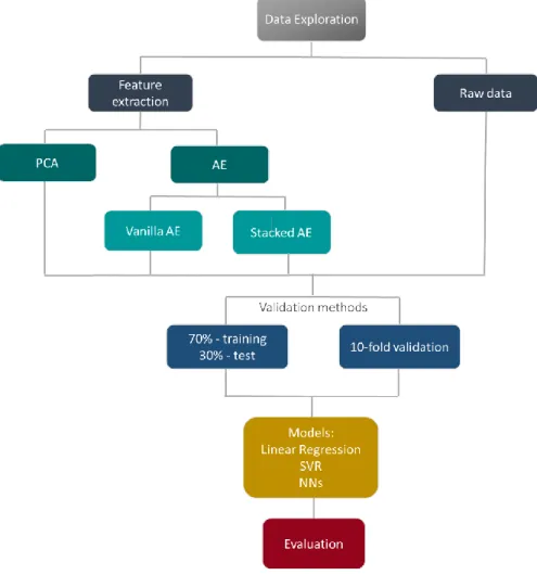
4.1 RESEARCH METHODOLOGY MAIN STEPS ... 34
4.2 DATASET... 35
4.3 TECHNICAL RESEARCH TOOLS ... 36
4.4 INITIAL DATA COMPREHENSION ... 36
4.5 EXTRACTING FEATURES WITH PRINCIPAL COMPONENT ANALYSIS ... 37
4.6 EXTRACTING FEATURES WITH AUTOENCODER ... 40
4.6.1 Training Vanilla autoencoder ... 40
4.6.2 Visualizing features obtained by training Vanilla autoencoder ... 41
4.6.3 Training Stacked autoencoder and feature visualization... 42
4.7 EVALUATION METHOD ... 44
4.7.1 Linear Regression ... 44
4.7.2 Support vector regression ... 45
4.7.3 Neural Network model ... 46
4.7.4 Validation method ... 46
CHAPTER 5 RESULTS AND DISCUSSION ... 48
5.1 RAW DATA OUTCOME ... 48
5.2 PCA OUTCOME ... 49
5.3 AUTOENCODER OUTCOME ... 51
5.4 STACKED AUTOENCODER OUTCOME ... 53
5.5 COMPARATIVE ANALYSIS OF RESULTS FROM DIFFERENT INPUTS ... 55
CHAPTER 6 CONCLUSIONS AND FUTURE WORK ... 57
BIBLIOGRAPHY ... 59 APPENDIX A ... 69 APPENDIX B ... 70 APPENDIX C ... 71 APPENDIX D ... 72 APPENDIX F ... 74
vii
List of Figures
Figure 1.1 Distribution of published papers that use deep learning in subareas of health informatics ... 4
Figure 2.1 Illustration of the mathematical model of a biological neuron – single perceptron ... 7
Figure 2.2 Multilayer perceptron ... 8
Figure 2.3 Sigmoid activation function ... 10
Figure 2.4 Hyperbolic tangent activation function ... 10
Figure 2.5 ReLU activation function ... 11
Figure 2.6 The output of the Softmax function for 4 classes ... 11
Figure 2.7 The gradient of the loss function ... 13
Figure 3.1 Autoencoder architecture ... 16
Figure 3.2 Boltzmann machine ... 19
Figure 3.3 Restricted Boltzmann machine ... 19
Figure 3.4 Training a Stacked Autoencoder ... 21
Figure 3.5 Sparse Autoencoder ... 24
Figure 3.6 Denoising autoencoder ... 26
Figure 3.7 Denoising effect ... 26
Figure 3.8 Variational autoencoder ... 29
Figure 3.9 Convolution and pooling in CNN ... 30
Figure 3.10 Convolutional autoencoder ... 31
Figure 3.11 The unfolded recurrent neural network ... 32
Figure 4.1 The core block diagram of the proposed methodology ... 34
Figure 4.2 Correlation matrix of Parkinson’s patient dataset presented with the heatmap ... 37
Figure 4.3 Visualization of the cumulative proportion of total variance explained by PCA ... 38
Figure 4.4 Scatter plot of the three-dimensional representation produced by taking the first three principal components obtained from different sets of input attributes with the color specification of total_UPDRS scores ... 39
Figure 4.5 Training autoencoders of different architectures ... 41
Figure 4.6 Scatter plots of three-dimensional codes produced by training autoencoders based on different sets of input attributes with the color specification of total_UPDRS scores ... 42
Figure 4.7 Scatter plots of three-dimensional codes produced by training the 19-15-10-5-3 stacked autoencoder with the color specification of total_UPDRS scores ... 43
Figure 4.8 Neural network architectures used in supervised learning ... 46
Figure 5.1 Training process of the 20-5-NN model with different number of epochs fed with raw data ... 49
viii
Figure 5.4 Training stacked autoencoders of different architectures ... 55
Figure Appendix D-1 Scatter plot of total_UPDRS vs motor_UPDRS ... 72 Figure Appendix D-2 Scatter plot of the three-dimensional representation produced by taking the first three
principal components obtained from different sets of input attributes with the color specification of
motor_UPDRS scores ... 72 Figure Appendix E-1 Visualization of training autoencoders with different hyperparameters and number of epochs
... 73 Figure Appendix F-1 Scatter plots of the three-dimensional codes produced by training autoencoders of different
ix
List of Tables
Table 3.1 Variants of the gradient descent (GD) based on the amount of data ... 23
Table 3.2 Extensions of the gradient descent ... 23
Table 3.3 Literature review on Autoencoders covered in this thesis ... 32
Table 4.1 Variable description of Parkinson’s telemonitoring dataset ... 35
Table 5.1 Model performance and computation time using patient data represented by original descriptors ... 48
Table 5.2 Model performance and computation time using patient data represented by features obtained with PCA ... 49
Table 5.3 Model performance and computation time using patient data represented by features obtained with autoencoders of different architectures ... 51
Table 5.4 Model performance and computation time using patient data represented by features obtained with stacked autoencoders ... 53
Table 5.5 Total UPDRS scores prediction results using patient data represented by 19 original descriptors and pre-processed by principal component analysis, vanilla and stacked autoencoders ... 55
Table Appendix A-1 Descriptive statistics of Parkinson’s patient dataset ... 69
Table Appendix B-1 Correlation coefficients between variables in Parkinson’s patient dataset ... 70
Table Appendix B-2 Top-10 the most correlated variables ... 70
Table Appendix C-1 Proportion of the variance explained by principal components obtained via transformation of 16 vocal attributes ... 71
Table Appendix C-2 Proportion of the variance explained by principal components obtained via transformation of 19 original attributes ... 71
Introduction
1.1 Motivation
This thesis is aimed at exploring capabilities of different types of autoencoders in extracting useful features for the representation of Parkinson's disease patients and comparing its performance in supervised learning with the representation obtained using principal component analysis (PCA) technique and with the raw data.
Like PCA, autoencoders can provide a solution for learning a lower dimensional latent representation but unlike PCA, they learn non-linear transformations. Having shown better performance in training since 2006 when it was first applied to MNIST dataset (Hinton & Salakhutdinov, 2006), it seems appealing to apply this technique, especially when a problem to be solved is characterized by complex interrelationships between variables.
1.2 Background
1.2.1 Theoretical framework
An autoencoder is an artificial neural network which is trying to reconstruct the input in the output while being trained (Goodfellow, Bengio, & Courville, 2016). It belongs to the class of unsupervised learning algorithms (Baldi, 2012), so it finds patterns in a dataset by learning the internal structure and features of data.
Initially, autoencoders were primarily viewed as a tool for dimensionality reduction and feature learning (Goodfellow et al., 2016). With the emergence and development of contemporary deep learning, autoencoders are considered as an effective way in pre-training neural networks (Hinton & Osindero, 2006; Bengio et al., 2007).
The idea of autoencoders was first associated with the resurgence of interest in back-propagation algorithm (Rumelhart, Hinton, & Williams, 1986). In 1988, again as a part of the
Chapter 1 Introduction
2
historical background of neural networks, the term "auto-association" was used in studying multilayer perceptron (Bourlard & Kamp, 1988).
A 1989 paper contributed to further study of autoencoders by examining the auto-associative case in detail and demonstrating how, using the backpropagation algorithm, learning occurs without a priori knowledge of data structure (Baldi & Hornik, 1989). This paper also showed that when an activation function is linear, the auto-associative case is a special case of PCA (Baldi & Hornik, 1989).
In 1994, Hinton and Zemel's paper introduced a new way of training autoencoders to study non-linear representations (Hinton & Zemel, 1994). Here, the term autoencoder was used instead of auto-association, although the terminology associated with the concept has continued to evolve over time.
The next milestone dates back to 2006 when several papers on the subject were published. The paper (Hinton & Osindero, 2006) marked the beginning of contemporary deep learning era (Wang & Raj, 2017) and introduced a deep belief network with layer-wise pretraining method. The work of (Hinton & Salakhutdinov, 2006) explored how a multi-layered neural network could be pre-trained one layer at a time by fine-tuning deep autoencoder using backpropagation. Here, feature learning for dimensionality reduction purpose was conducted by both, autoencoder and PCA, resulting in outperformance of autoencoders (Hinton & Salakhutdinov, 2006). This paper was one of the inspirational sources for the thesis.
The idea of layer-wise pretraining has been exploited in several studies where further explanation of the pre-training mechanism was provided with some proposed refinements (Bengio et al., 2007; Bengio, 2009; Vincent et al., 2010) but the stem idea came from the original work on deep belief networks. The main principle is that to obtain a low-dimensional representation, each layer is trained at a time by optimizing a local unsupervised criterion to produce a useful higher-level representation based on the input from the below layer with the expectation to improve the generalized representation. As a result, several autoencoders are stacked together. This architecture is often referred as stacked autoencoder.
Using autoencoders as data compressors is considered a classical approach (Rifai et al., 2011). Modern architectures of autoencoders is mostly associated with so-called overcomplete architectures with the code size larger than the input. Such autoencoders require the
3
introduction of special regulators to avoid useless reconstruction (Goodfellow et al., 2016). Regularized autoencoders will be discussed in the third chapter.
1.2.2 Autoencoders in medical data research
The subsection 1.2.1 describes the important milestones that form the body knowledge about autoencoders. The mentioned research papers provide a contextual approach to the scientific understanding of the concept. The subject of interest covered by this thesis is applying the autoencoder algorithm for Parkinson's disease patient data and comparing its feature extraction capabilities with other methods.
Since then as deep machine learning techniques have shown their effectiveness in both, supervised and unsupervised tasks, they proved to be well suitable to medical big data to extract useful knowledge from it (Litjens et al., 2017). There are several interesting papers related to the use of autoencoders in the field of medicine. One of the greatest inspirations for the present work was a study conducted by a research team at Mount Sinai Hospital in New York City in 2015. Based on the electronic health records (test results, doctor visits, and so on), a patient´s representation was derived using the stacked autoencoder architecture and called "Deep Patient" (Miotto et al., 2016). Without any expert instruction, Deep Patient discovered hidden patterns in the hospital data that can predict the patient's future with respect to the development of certain diseases. The results obtained using Deep Patient representation were better than when using raw patient's data or representation obtained using PCA (Miotto et al., 2016).
A similar approach for feature extraction with subsequent use in supervised learning is described in the paper (Zafar et al., 2016). The proposed method, called SAFS, used the stacked autoencoder for a higher-level representation of the most vulnerable demographic subgroup of patients to predict risk factors for hypertension. The results showed that SAFS approach and representation learning outperform the models with unrepresented input. This paper demonstrated how deep architectures can be applied to a specific precision medicine problem. Of particular interest is a recent paper where a stacked autoencoder and softmax classifier were used to diagnose Parkinson's disease (Caliskan et al., 2017). As in previous studies, the framework involved unsupervised learning to extract representation features that served as an input for supervised learning while a softmax classifier was built for prediction purposes.
Chapter 1 Introduction
4
This paper showed how the data dimension can be reduced with an autoencoder, and thereby improve the predictive power of a classifier.
1.3 Study relevance
Deep learning is an active research area. Many interesting papers are constantly appearing in journals. In healthcare, they are primarily pertinent to medical image analysis (Litjens et al., 2017). Nevertheless, the flow of medical data is much more diverse and not limited to images. Figure 1.1 shows an increasing number of publications on deep learning in healthcare sub-areas.
Figure 1.1 Distribution of published papers that use deep learning in subareas of health informatics Source: (Ravi et al., 2017)
In papers that provide a review of deep learning in medicine, autoencoders are referred as one of the commonly used deep learning architectures along with other deep learning techniques (Ravi et al., 2017; Litjens et al., 2017). The main idea of their use is to capture useful properties for the representation, whether it is an image or a numeric vector of an observation.
Parkinson's disease is a degenerative neurological disorder, the second most common after Alzheimer's disease. About 5 million people suffer from Parkinson's disease worldwide (Gibrat et al., 2009). Some motor symptoms can drastically affect the quality of the patient's daily life (Bryant et al., 2015). Diagnosis of the disease in the early stages can significantly improve the plan for necessary treatment, and thus, maintain the quality of life (Challa et al., 2016). A great interest in detecting markers for the diagnosis of the disease is related to the fact that this can be done in the preclinical stage (Postuma & Montplaisir, 2009). Parkinson's disease is
5
known for causing disturbances of varying degrees in the production of vocal sounds (Asgari & Shafran, 2010). Voice recording and speech tests can be an effective non-invasive tool for diagnosis (Tsanas et al., 2010).
Machine learning algorithms have been already used to extract useful information from patients' speech and predicting the severity of Parkinson's disease (Nilashi et al. , 2016; Caliskan et al., 2017). Nevertheless, the improvement of algorithms themselves, including those related to deep learning, provides the ground for continuing studies of patients' speech data to further improve the overall prognostics and develop applications for home-based assessment or telemonitoring Parkinson's disease outside of hospital settings (Asgari & Shafran, 2010).
Parkinson's patient voice data is measurable but some characteristics are indecipherable for the human ear, especially on early stages of the disease (Rouzbahani & Daliri, 2011). Identifying and measuring speech patterns in patients and comparing them with healthy people is thereby becoming one of the central tasks in the study of voice data. In this regard, applying deep techniques, in particular, autoencoders seems to be adequate and promising since these methods have already proved effective in capturing silent features in complex data (Ravi et al., 2017).
1.4 Objectives
The main goal of this study is to explore whether it is possible to improve the Parkinson's patient representation by extracting useful features from a range of biomedical voice measurements using an autoencoder. To achieve the main goal, the following specific objectives were defined:
1. Systematize the knowledge base of autoencoders to provide the background and establish a sense of structure that guides the research.
2. Apply unsupervised learning techniques to train neural networks for the Parkinson's patient representation.
3. Provide sensitivity analysis when using different types of autoencoders, PCA, and raw data.
4. Compare the performance of representations obtained by the autoencoder, PCA and raw data in the supervised learning.
Chapter 2
Neural networks:
Definitions and basics
The aim of this chapter is to provide an essential background of artificial neural networks for a better intuitive understanding of concepts and further exploration of autoencoders.
2.1 Introduction to artificial neural networks
Inspired by biological mechanisms for the processing of natural signals in the human brain, artificial neural networks (ANN) were the subject of research since the mid-20th century (Deng et al., 2014). The principal unit of the artificial neural network is a node by analogy with the biological brain neuron. Connections between neurons in ANN also simulate interconnections between neurons in the brain (Gibson & Patterson, 2017). Neurons are exchanging signals between one another forming a dense and complex network.
The term "neural network" appeared in the middle of XX century. In 1943, McCulloch and Pitts introduced a simplified model of a neuron in their paper (McCulloch & Pitts, 1943) which is considered the beginning of the computational theory of brain activity (Piccinini, 2004). Later, in the 50’s, Frank Rosenblatt developed a neural network model based on mathematical algorithms (Rosenblatt, 1958). Like its biological prototype, an artificial neuron can learn by adjusting parameters that describe synaptic conductivity. This model has laid the foundation for studies of neural networks as biological processes in the brain, and use of neural networks as an artificial intelligence method for solving various applied problems (Wang & Raj, 2017).
2.1.1 Single perceptron
The simplest form of a neural network was given the name of a perceptron back in Rosenblatt's work. The perceptron was originally conceived as a simplified mathematical model of neuronal processes in the brain: "The perceptron is designed to illustrate some of the fundamental properties of intelligent systems in general, without becoming too deeply enmeshed in the
7
special, and frequently unknown, conditions which hold for particular biological organisms" (Rosenblatt, 1958).
Figure 2.1 shows a perceptron and zooms in detail how data is processed by neurons. The perceptron is considered a feed-forward network. The term forward is used to indicate the direction of the information flow in neural networks – from the input to the output layer without cycles. The perceptron takes the input data 𝒙𝒊 and proceeds it to the neuron (cell body). The incoming signal is multiplied by a weight value 𝒘𝒊 that is assigned to each input 𝒙𝒊. The neuron processes weighted inputs by summing up to one value. At this stage, a bias or offset term, referred to as 𝒃 or 𝒘𝟎 in machine learning models, is added. The bias has a value of 1 and ensures that different functions are computable by shifting them to get a better approximation. Finally, an output signal is produced by performing a mathematical operation on the above result using the activation function 𝒇(𝒙).
Figure 2.1 Illustration of the mathematical model of a biological neuron – single perceptron Source: adapted from (Karpathy, 2015)
2.1.2 Multilayer perceptron
In 1969, Minsky and Papert published the book "Perceptrons" where they expressed their scepticism about the perceptron, in particular, of its incapability to learn non-linearly separable boolean XOR function (Minsky & Papert, 1969). This publication is now regarded in literature as the beginning of so-called "AI winter", the period that followed a massive wave of interest to neural networks. Minsky and Papert didn't merely show limitations of the perceptron but argued that a solution to XOR problem can be found by training networks with multiple layers, although a practical study of such networks happened a little later.
Chapter 2
Neural networks: Definitions and basics
8
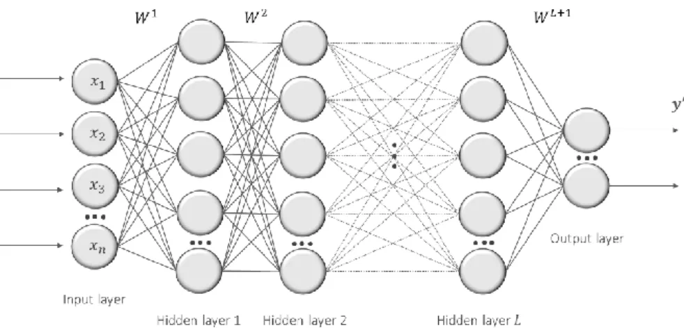
One or more neurons in the hidden layer connected only with the input and output form a single-layer neural network. Increasing the number of neurons in a single single-layer results in a shallow neural network architecture. By stacking one-layer neural network upon another and feeding the successor layers with the output from previous layers one can get a deeper, fully connected neural network which is also known as a multilayer perceptron (Figure 2.2).
Figure 2.2 Multilayer perceptron
A multilayer perceptron uses the feed-forward mechanism in information processing. The idea of feed-forward network is to approximate some function 𝒇(𝒙) and map the input represented by a vector 𝒙 ∈ ℝ𝒏 to a target 𝒚. The network defines the mapping 𝒚′ = 𝒇(𝒙, 𝒘, 𝒃) and learns the values of parameters 𝒘 and 𝒃 resulting in the best function approximation. As it was examined in subsection 2.2.1 each neuron's output will be computed by activating the weighted sum of the previous layer input. Equation (2.5) represents this mathematically:
𝑎𝑗 = 𝑓(∑ 𝑤𝑖𝑗𝑥𝑖 + 𝑏𝑗),
𝑛 𝑖=1
(2.1)
where 𝒇 is an activation function; 𝒘𝒊𝒋 – weight for the connection of input 𝒙𝒊 to a neuron 𝒋;
𝒃𝒋– bias term of the corresponding neuron.
The presence of several hidden layers requires the introduction of an additional nomenclature (for the convenience of designation in vectorized form):
𝑧 = 𝑊𝑥 + 𝑏 (2.2)
𝑎 = 𝑓(𝑧), (2.3)
where 𝑾 ∈ ℝ𝒎𝒙𝒏, 𝒃 ∈ ℝ𝒎, 𝒎 is a number of units in a layer, and 𝒇 is applied stepwise,
9
𝑓(𝑧) = 𝑓([𝑧1, 𝑧2, … 𝑧𝑚]) = [𝑓(𝑧1); 𝑓(𝑧2); … 𝑓(𝑧𝑚)] (2.4)
For subsequent stacked layers, a superscript will be used to denote each layer and parameterize each layer connection. So, the equation takes the following form:
𝑎𝑘𝑙 = 𝑓(∑ 𝑤𝑘𝑗𝑙 𝑎𝑗𝑙−1
𝑗
+ 𝑏𝑘𝑙), (2.5)
where each weight has two indices: 𝒋 indicates an emitting node and 𝒌 – a receiving node. The mathematical explanation of the feed-forward process in a multilayer perceptorn make it clear that increasing the number of layers makes sense only when using non-linear activation functions, otherwise, several layers of linear perceptrons can be collapsed into one due to the linearity of the entire circuit of computations (Ng, Katanforoosh, & Mourri, 2017b).
2.1.3 Activation functions
In the original perceptron, the activation function was a simple threshold operator. Linear functions have also been exploited as activation functions in neural networks (Baldi & Hornik, 1989). In modern networks, however, activation functions are most often referred to as non-linear functions. Adding nonnon-linearity to the network allows it to learn more complex functional mappings from data and avoid constraints associated with linear functions.
There are several commonly used activation functions in neural networks. The following subsections discuss how exactly each of the functions proceeds the linear combination of weighted inputs to produce non-linear decision boundaries in hyperplanes.
2.1.3.1 Sigmoid activation function
The sigmoid has a mathematical form as shown by equation (2.1). It maps a real number into the interval between 0 and 1 (Figure 2.3).
Chapter 2
Neural networks: Definitions and basics
10
𝜎(𝑥) = 1
1 + 𝑒−𝑥 (2.6)
Figure 2.3 Sigmoid activation function
2.1.3.2 Hyperbolic tangent activation function
The hyperbolic tangent or tanh nonlinearity is shown by equation (2.2). It squashes a real-valued number to the range between -1 and 1. Unlike the sigmoid, its output is zero-centred (Figure2.4).
𝑡𝑎𝑛ℎ(𝑥) =1 − 𝑒
−2𝑥
1 + 𝑒−2𝑥 (2.7)
Figure 2.4 Hyperbolic tangent activation function
2.1.3.3 Rectified Linear Unit (ReLU) activation function
This function became popular after showing its effectiveness in training some types of neural networks (Nair & Hinton, 2010), as well as being faster for training larger networks (Krizhevsky, Hinton, & Sutskever, 2012). The ReLU returns zero if the value of the argument is negative, and raw output otherwise (2.3). In other words, the activation is generated at zero. This effect is shown on Figure 2.5.
The rectifying neurons have been explored in the paper (Glorot, Bengio, & Bordes, 2011). These neurons, according to the study's authors, are more biologically authentic and perform equally or better in comparison to sigmoid and hyperbolic tangent networks.
11
𝑅𝑒𝐿𝑢 = 𝑚𝑎𝑥(𝑥, 0) (2.8)
Figure 2.5 ReLU activation function
2.1.3.4 Softmax activation function
The softmax function is usually applied at the output level of a neural network when dealing with multinomial logistic regression where the dependent variable has more than two levels (albeit it can also be used for a binary classifier). The softmax function squashes outputs of each unit to the range [0, 1] so, that the total sum of outputs is equal to 1. The result of softmax is equivalent to the categorical probability distribution (Hinton, Srivastava, & Swersky, 2012). The mathematical form of the softmax function for 𝒌 classes is represented by equation (2.4).
𝑠𝑜𝑓𝑡𝑚𝑎𝑥(𝑥𝑗) = 𝑒
𝑥𝑗
∑𝑘 𝑒𝑥𝑘 𝑘=0
, 𝑓𝑜𝑟 𝑗 = 1 … 𝐾, (2.9)
The output of the softmax function might look like a matrix of probabilities (Figure 2.6). For example, let the target have 4 labels (assuming indexing from zero) and let's take 4 training samples. The resulting prediction matrix will have the probabilities of belonging to a class. The indicator target matrix assigns a class for each sample.
Original target (label) Probabilities predicted Indicator target matrix
[ 0 1 2 3 ] [ 0.6 0.1 0.2 0.1 0.1 0.7 0.1 0.1 0.2 0.1 0.5 0.2 0.1 0.1 0.1 0.7 ] [ 1 0 0 0 0 1 0 0 0 0 1 0 0 0 0 1 ]
Chapter 2
Neural networks: Definitions and basics
12
2.2 Training artificial neural networks
The learning algorithm used in the Rosenblatt's perceptron for the binary classification was based on the Perceptron convergence theorem. The idea was to find the upper and lower bounds along the length of the weight vector by updating the weights accordingly (Haykin, 2008). An important variation of the perceptron training algorithm was introduced by (Widrow & Hoff, 1960) who developed a model, called ADALINE, based on the least-mean-square (LMS) algorithm. The main difference from the perceptron is the way the output of a neural system is used in the learning rule, known as Delta rule. These two were the first training algorithms specific to single-layer neural networks. Minsky and Pitts’s work showed that these techniques do not work for multilayer networks but didn’t provide a solution to the problem of how to adjust weights in hidden layers that are not connected to the output. The issue of training multilayer networks remained open until the idea of propagating the error in the opposite direction of the forward process with the explanation of reverse calculations became the subject of close examination in several works since the early 1970s.
2.2.1 Backpropagation
A valuable contribution to overcoming restrictions of previous algorithms for training multilayer networks was first made by Paul Werbos, who proposed a backpropagation training technique published in his PhD thesis (Werbos, 1974). This work remained almost unknown in the scientific community until the method was again explored by David Parker who published his findings in the technical report (Parker, 1985). Finally, in 1986, a well-known paper on backpropagation was published by Geoff Hinton, David Rumelhart and Ronald Williams (Rumelhart et al., 1986). The idea conceived by people in the past was concisely stated and led to a clear framework which enhanced its popularization (Widrow & Lehr, 1990). The paper of 1986 showed that backpropagation worked much faster than previous approaches to learning. It has been eventually considered the starting point of the contemporary Deep learning theory (Wang & Raj, 2017; Beam, 2017).
Backpropagation belongs to the iterative optimization algorithms that progressively improve the results with respect to the objective function. The objective function (𝑱), also called loss or cost function, is a difference between estimated (𝒚′) and true values (𝒚) of the target. In
13
other words, it shows how much different our mappings from actual values are. The generic relationship can be denoted as follows:
𝐽 = 𝑦 −𝑦′ (2.10)
In applied tasks, different loss functions are used depending on the problem at hand. The most used ones are cross-entropy and mean squared error or mean absolute error (Goodfellow et al., 2016).
Changing the parameters towards the optimal solution minimizing the cost function is basically what the training process is:
𝐽 = 𝑚𝑖𝑛(𝑓(𝑥, 𝜃)), (2.11)
where 𝜽 is parameters 𝒘 and 𝒃.
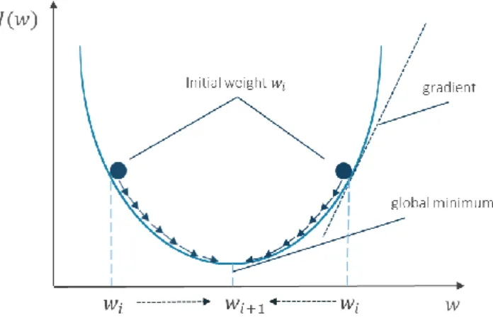
To find an optimal combination of parameters by checking all possible combinations is a very exhaustive process. The point is to figure out which way is downhill to understand whether to increase or decrease the value of weights to minimize the cost function. Knowing the direction in which to move, rather than applying countless combinations of weights, leads to a faster optimization. This numerical estimation is called a gradient descent. Graphically, this is reflected by the slope of the loss function at a certain point corresponding to a specific weight value 𝒘𝒊 (Figure 2.6).
Figure 2.7 The gradient of the loss function Source: adapted from (Raschka, 2015)
This way, the change in the loss function at each point with respect to the parameter change is nothing other than a derivative of the function with respect to weights. Parameters will be
Chapter 2
Neural networks: Definitions and basics
14
adjusted incrementally to a step size value 𝜶 which is called learning rate, by increasing (2.12) or decreasing (2.13) in a direction of the gradient.
𝑤𝑖+1← 𝑤𝑖 + 𝛼 𝜕𝐽 ∂𝑤𝑖 (2.12) 𝑤𝑖+1← 𝑤𝑖− 𝛼 𝜕𝐽 ∂𝑤𝑖 (2.13)
Since the derivative of the function is a product of derivatives of several terms, the concept of a total derivative is applied. The process becomes apparent when applying the chain rule to calculate the derivative of each component. First, the derivative of the cost function with respect to the parameters of the last hidden layer are calculated. The gradients for the output layer directly affect the cost function. Using the chain rule, the derivative of the cost function with respect to the weights in the last layer is a result of three components. The first component is a derivative of the cost function with respect to the output. Its calculation depends on the exact formula of the chosen cost function. The second component is a derivative of the activation function which will be assumed as sigmoid 𝝈 for ease of presentation. The third component is a derivative of linear function and it corresponds to the activation from the previous layer. This is reflected by equation 2.14:
𝜕𝐽 ∂𝑤𝑗𝑘𝐿 = 𝜕𝐽(𝑦′, 𝑓 (𝑧𝑗𝐿(𝑤𝑗𝑘𝐿))) 𝜕𝑤𝑗𝑘𝐿 = 𝜕𝐽 𝜕𝑦′∗ 𝜕𝑎𝑗𝐿 𝜕𝑧𝑗𝐿∗ 𝜕𝑧𝑗𝐿 𝜕𝑤𝑗𝑘𝐿 (2.14)
where 𝑳 is the last layer in the sequence 𝑙 = 1, 2, … 𝐿.
According to common conventions, the symbol 𝜹𝒍 is used to denote the error associated with the layer 𝒍. This is the value that network parameters will be adjusted to. The partial derivative of the error function with respect to weights in the final layer has a following form:
𝜕𝐽 ∂𝑤𝑗𝑘𝐿 = 𝛿 𝐿∗ 𝜕𝑎𝑗 𝐿 𝜕𝑧𝑗𝐿 ∗ 𝜕𝑧𝑗𝐿 𝜕𝑤𝑗𝑘𝐿 = 𝛿 𝐿𝑎 𝑗𝐿−1 (2.15)
For the hidden layers, the chain rule for multivariate functions is applied again: 𝜕𝐽 ∂𝑤𝑗𝑘𝑙 = 𝜕𝐽 𝜕𝑎𝑗𝑙∗ 𝜕𝑎𝑗𝑙 𝜕𝑧𝑗𝑙∗ 𝜕𝑧𝑗𝑙 𝜕𝑤𝑗𝑘𝑙 = 𝜕𝐽 𝜕𝑎𝑗𝑙𝜎 ′(𝑧 𝑗𝑙)𝑎𝑘𝑙−1 (2.16)
The derivative of the cost with respect to the activation 𝝏𝒂𝝏𝑱
𝒋
𝒍 is a part of the input to the
15 𝜕𝐽 ∂𝑎𝑗𝑙 = ∑ 𝜕𝐽 𝜕𝑧𝑚𝑙+1∗ 𝜕𝑧𝑚𝑙+1 𝜕𝑤𝑗𝑙 𝑚 = ∑ 𝛿𝑚𝑙+1 𝑚 𝑤𝑚𝑗𝑙+1 (2.17)
In the propagated sequence all deltas are connected in the recursive formula where the delta of the previous layer is a function of the delta in the subsequent layer:
𝛿𝑗𝑙 = (∑ 𝛿𝑚𝑙+1
𝑚
𝑤𝑚𝑗𝑙+1)𝜎′(𝑧𝑗𝑙) (2.18) The generalized formula for updating the weights will take a form:
𝛥𝑤𝑗𝑘𝑙 = 𝛼𝜕𝑓(𝑥, 𝜃)
∂𝑤𝑗𝑘𝑙 (2.19)
Summarizing the backpropagation algorithm, the following steps can be identified:
1. Forward path. Computing the sequence of inputs and outputs in each of the layers by summing weighted inputs and adding nonlinearity.
2. Backward path. Obtaining an error term in the final layer and backpropagating it to the hidden layers by reapplying equation (2.18).
3. Combining all the gradients in each layer to get the total gradient.
Chapter 3
Autoencoder framework
This chapter provides an overview of autoencoders and their varieties. The goal is to explain the difference between autoencoders based on principles of how they learn the representation of data rather than focusing on the mathematical explanation of parameters introduced for this purpose.
3.1 Overview
The idea behind autoencoders is to reconstruct the input data in the output with the least possible distortion (Baldi, 2012). Formulated this way, it may seem useless but the expectation is that useful properties of the input will be extracted in the course of training.
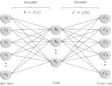
An autoencoder is respectively composed by three components: an encoder, code, and decoder. The encoder compresses the input and generates the code, the decoder reconstructs the input based on the code (Figure 3.1). The training process is similar to training feedforward neural network via backpropagation (Goodfellow et al., 2016). Autoencoders by their nature are lossy which means that the output will degrade compared to the original input. The goal of training is to minimize the reconstruction error.
17
3.2 Autoencoder algorithm
Each input in the autoencoder is represented by a vector 𝒙 ∈ ℝ𝒏of a dimension 𝒏 equal to
the input size. The autoencoder takes the input and first maps it to a hidden representation or code through a deterministic mapping, called the encoder which can be viewed as a function:
ℎ = 𝑓𝜃(𝑥) = 𝜎(𝑥𝑊 + 𝑏), (3.1)
where 𝜽 = {𝑾, 𝒃} ; 𝑾 ∈ ℝ𝒎𝒙𝒏 is a weight matrix; 𝒃 ∈ ℝ𝒎 is a bias vector; 𝒇
𝜽(𝒙) – the
encoder; 𝝈 is an activation function1.
The hidden representation is mapped back with the decoder reproducing the output layer 𝒙′ ∈ ℝ𝒏 of the same dimension 𝒏 as the input. This process can be written as a function:
𝑥′ = 𝑔𝜃′(ℎ) = 𝜎(ℎ𝑊′ + 𝑏′), (3.2)
where 𝜽′ = {𝑾′, 𝒃′}; 𝒈𝜽′(𝒉) – the decoder.
One of the approaches to constrain the weight matrix of the decoder 𝑾′ is to transpose the encoder weight matrix 𝑾′= 𝑾𝑻. This is referred to as tied weights. The use of tied weights is optional and some experiments with untied weights have yielded similar results (Vincent et al., 2010).
3.3 Parametrization of Autoencoder
To train an autoencoder, several parameters must be pre-set. These are parameters that determine the architecture of an autoencoder (code size, number of layers) and training parameters (loss function, activation function at each layer, optimizer, regularizer).
3.3.1 Code size
The code size is a number of units in the middle layer of an autoencoder or the last layer of the encoder. By the size of the code, autoencoders can be classified into two groupings - undercomplete and overcomplete autoencoders.
Chapter 3
Autoencoder framework
18 3.3.1.1 Undercomplete Autoencoders
Undercomplete autoencoders have a code size smaller than the input size. These autoencoders are designed to capture useful features in the data and reduce its dimensionality by representing the whole population with captured silent features. In this case, the network is encouraged to learn some sort of compression.
3.3.1.2 Overcomplete Autoencoders
The dimensionality reduction argument is built on the assumption that the code dimension is smaller than the input. Nevertheless, even with the opposite statement, an autoencoder can learn useful information about the data structure by imposing some constraints on the activity of the hidden representations (Ng, 2011). When the architecture is properly adjusted by adding the regularization terms, the autoencoder gains other qualities besides its capacity to copy the input to the output. These autoencoders will be considered in section 3.3.6 when different types of regularization are introduced.
3.3.2 Number of layers
Depending on the number of hidden layers, autoencoders can be divided into deep and shallow. A shallow autoencoder has just one hidden layer and it can be viewed as a Restricted Boltzmann machine (Hinton, 2012c), especially when trained with contrastive divergence (Hinton, 2002). The first deep architectures were trained precisely as stacked RMBs. In the following subsections, the evolution from shallow to deep architectures is considered, and the main difference between stochastic and deterministic algorithms is defined.
3.3.2.1 Restricted Boltzmann machine
The Boltzmann machine was introduced in the paper (Ackley, Hinton, & Sejnowski, 1985) with subsequent variations that have surpassed their original version (Goodfellow et al., 2016), and underlie the modern deep learning (Heaton, 2015).
A Boltzmann machine is a kind of fully connected neural networks that can be considered as a stochastic generative variant of the Hopfield network (Hopfield, 1982) in which neurons are both, input and output. The Boltzmann machine consists of two layers – visible 𝒗 ∈ ℝ𝒏 and
19
hidden 𝒉 ∈ ℝ𝒌 (Figure 3.2). The inputs are binary vectors and the learning algorithm is based
on maximum likelihood (Goodfellow et al., 2016).
Figure 3.2 Boltzmann machine
One of the varieties of Boltzmann machines is a Restricted Boltzmann machine (RBM) which was introduced by Paul Smolensky under the name harmonium (Smolensky, 1986). The main difference is that there are no connections between neurons in the same layer (Figure 3.3).
Figure 3.3 Restricted Boltzmann machine
The training algorithm consists of several forward and backward passes in a fashion of training a feedforward network with the difference that an RBM does not produce the output. The hidden layer is used to model the input data, and then, to reconstruct it in the visible layer. This implies a bi-directional relationship between layers (Hinton, 2012b) which is reflected by so-called bipartite graph (Figure 3.3). The fact that RBMs are undirected and neurons are activated probabilistically makes them a special case of Markov networks (Hinton, 2012a).
Chapter 3
Autoencoder framework
20 3.3.2.2 Deep belief network
In 2006, the paper (Hinton & Osindero, 2006) demonstrated how several RBMs can be stacked together and trained in a greedy manner to form a deeper structure, called Deep Belief Network (DBN). When two layers of the RBM are part of a deeper neural network, the output of the hidden layer is passed as the input to the next hidden layer, and from there through as many hidden layers as defined. These feed-forward movements form an architecture that resembles an autoencoder, however there is an essential difference between them. The goal of training a DBN is to reproduce the distribution of input data based on activations in the hidden layer using a stochastic approach, whereas an autoencoder is deterministically learning the representation of the input data. In other words, the hidden layer of a DBN is a probabilistic distribution among the hidden variables and the hidden layer of an autoencoder is a representation of the input data.
The Deep Belief Network is a hybrid involving both, directed and undirected connections. The presence of directions distinguishes DBNs from Deep Boltzmann machines (Salakhutdinov & Hinton, 2009) that are fully undirected.
DBNs are not commonly used in the modern architectures but they played a fundamental role in the history of deep learning (Goodfellow et al., 2016) and considered the predecessors of contemporary generative algorithms (Salakhutdinov, 2015).
3.3.2.3 Stacked autoencoder
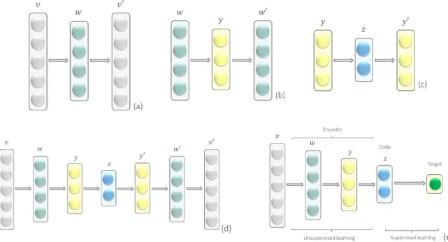
The first deep networks were trained in a greedy layer-wise manner. The papers (Hinton & Salakhutdinov, 2006; Bengio et al., 2007) showed how using this method, one can obtain the representation that yields a better performance in the supervised learning. This approach underlies the stacked autoencoder where several codes of a vanilla encoder are combined into a more complex structure (Figure 3.4).
21
Figure 3.4 Training a Stacked Autoencoder
The algorithm of a stacked autoencoder can be described as follows:
1. Each layer is trained at a time to preserve as much information of input as possible (Figure 3.4 (a), (b), (c)).
2. The restoring layers 𝑣′, 𝑤′, 𝑦′ are discarded in each training procedure.
3. The weights of each hidden layer 𝒘, 𝒚, 𝒛 are fixed, and the next network is built based on data coming from the previous hidden layer which now acts as the input layer. 4. All hidden layers are combined forming a deep structure (Figure 3.4 (d)).
5. The fine-tuning of an entire network with respect to the final measure of interest is performed (Figure 3.4 (e)). Here, the transition from unsupervised to supervised learning is taking place. The full neural network processes all layers of the deep encoder as a single entity in such a way that weights are improved in the stacked autoencoder.
3.3.3 Loss function
The objective function evaluates the effectiveness of training neural networks. It returns a score that indicates how well a network performs. In the case of autoencoder, it measures how good the reconstruction is, reason why the term loss function is more adequate. Here, the commonly used loss functions will be considered, although the choice of functions is a lot richer.
Chapter 3
Autoencoder framework
22 3.3.3.1 Mean squared error loss function
Typically used for real-valued inputs, the function 𝑳 represents the sum of squared Euclidian distances between the input vector 𝒙 and reconstructed vector 𝒙′, as shown by equation (3.3).
𝐿(𝑥, 𝑔(𝑓(𝑥))) = 1 𝑛∑(𝒙′𝑖 − 𝑥𝑖) 2, 𝑛 𝑖=1 (3.3)
where 𝒈(𝒉) is the decoder output, 𝒉 = 𝒇(𝒙) is the encoder output or code.
When the input is real values [−∞; +∞] it is recommended to use a linear activation function in the last reconstruction layer (Larochelle, 2013).
3.3.3.2 Cross entropy loss function
Typically used for binary inputs, the loss function represents the sum of Bernoulli cross-entropies between two distributions:
𝐿(𝑥; 𝑔(𝑓(𝑥))) = −1
𝑛∑(𝑥𝑖𝑙𝑜𝑔 (𝑥′𝑖
𝑛
𝑖=1
) + (1 − 𝑥𝑖)𝑙𝑜𝑔 (1 − 𝑥′𝑖)) (3.4)
This function is also applicable when inputs belong to a range [0; 1] (Larochelle, 2013). In literature, one can be confronted with the term negative log likelihood. The cross entropy and negative log likelihood have different origins, from information theory and statistical modeling, respectively, while mathematically they are exactly the same (Gibson & Patterson, 2017).
3.3.4 Optimizer
These are the algorithms that try to find optimal values of mathematical functions used in training a neural network. The gradient descent algorithm is one of the optimization algorithms. It was considered in section 2.2.
There are different variants of the gradient descent algorithm with respect to the amount of data taken per update to compute the gradient, and extensions of the gradient descent based on different approaches to adapting the learning rate and selecting hyperparameters. We do not go into detail here and just summarize some of them (Table 3.1, Table 3.2).
23
Table 3.1 Variants of the gradient descent (GD) based on the amount of data Source: (Ruder, 2016)
Method Amount of data per update Update speed Memory usage Online learning
Stochastic GD one sample High Low Yes
Batch GD entire dataset Slow High No
Mini-batch GD around 50-250 samples Medium Medium Yes
Table 3.2 Extensions of the gradient descent Sources: (Portilla & Mosconi, 2017; Sokolov et al., 2017)
Method Description
Gradient descent Basic unmodified GD
Momentum Smooth updates. Tends to move in the same directions as on previous steps
Nesterov Momentum Update slows down before changing direction, making a small corrective jump based on
gradient
AdaGrad Separate learning rates for each dimension. Adaptive correction using squared gradient. Suits
for sparse data
RMSprop Learning rate adapts to latest gradient steps. EWMA2 applied to squared gradient AdaGrad
Adam Combines Momentum and individual learning rates. Use EMWA on 1st and 2nd moments
3.3.5 Regularization
A strategy aimed at improving the performance of algorithms not only on training but also on new data is known as regularization. There are various regularization methods that generally based on modifying the basic algorithm by adding some constraints. The following subsections discuss regularizers applicable to autoencoders.
3.3.5.1 Sparse autoencoder
The concept of sparsity was introduced in computational neuroscience (Olshausen & Field, 1997), and subsequently arose in different contexts: unsupervised learning of sparse features represented by the linear code (Ranzato et al., 2006); as a variant of DBNs in the context of convolutional networks (Ranzato, 2007; Lee & Ng, 2008; Mairal et al., 2009).
The overcomplete architecture of a sparse autoencoder allows a larger number of hidden units in the code, but this requires that for the given input, most of hidden neurons result in very
Chapter 3
Autoencoder framework
24
little activation (Ng, 2011). For each hidden node, the average activation value should be close to zero (in the case of sigmoid or to -1 when activation function is tanh). The neuron will be considered active if the output is close to 1, and otherwise – inactive (Ng, 2011).
What is the goal of having hidden units with most zeros? The idea is to make a neuron activated only for a small fraction of the training examples. Since the samples have different characteristics, the activation of neurons should not be held in the same fashion in all neurons and must be coordinated. The goal is to obtain a latent representation with many zeros and only a few non-zero elements that will represent the most protruding features (Figure 3.5).
Figure 3.5 Sparse Autoencoder
The training of a sparse autoencoder involves a penalty term on the code layer to reflect deviation from a desired sparsity. The penalty is added to the loss function modifying the error:
𝐿 (𝑥; 𝑔(𝑓(𝑥))) + 𝛺(ℎ), (3.5)
where 𝒈(𝒉) is the decoder output, 𝒉 = 𝒇(𝒙) is the encoder output or code, 𝜴(𝒉) is a sparsity penalty which is a log function (3.6; 3.7).
𝛺(ℎ) = ∑ 𝐾𝐿(𝑝||𝑝′𝑗) 𝑠
𝑗=1
, (3.6)
where 𝒑 is a sparsity parameter, typically a small value close to zero; 𝒑′𝒋 is the average
activation of hidden unit 𝒋, that is forced to approximate to 𝒑 ; 𝒔 is the number of neurons in the hidden layer; 𝑲𝑳 is Kullback-Leibler divergence (3.7) between a Bernoulli random variable with mean 𝒑 and a Bernoulli random variable with mean 𝒑′ (Ng, 2011).
25 𝐾𝐿(𝑝||𝑝̂𝑗) = 𝑝𝑙𝑜𝑔 𝑝
𝑝′𝑗+ (1 − 𝑝)𝑙𝑜𝑔
1 − 𝑝
1 − 𝑝′𝑗 (3.7)
The effects of introducing a sparse component into the network were explored and visualized using the MNIST dataset in the paper (Makhzani & Frey, 2014). In the hidden layer, only 𝒌 highest activities were kept. The results showed that with a higher level of sparsity, the network tended to capture local fragments of digits, and with decreasing values of 𝒌, it was forced to learn a more complete representation of each digit.
A method of creating a sparse representation by achieving true zero in the code layer was introduced in the paper (Glorot et al., 2011) where the ReLU activation function was used for this purpose. Researchers highlighted several reasons why a sparse representation might be appealing, thereby enriching the conceptual part about the need of sparsity – among others, information disentangling and efficient variable-size representation (Glorot et al., 2011). 3.3.5.2 Denoising autoencoder
The idea of training a network by adding noise was approached in the works (Gallinari et al., 1987) and (Lecun, 1987). Later, the denoising task was applied to more complex convolutional and recurrent networks (Seung, 1998; Jain & Seung, 2008) with continuing study of this parameterization on autoencoders (Alain & Bengio, 2014).
Denoising autoencoders are trained to map a noisy input to an output. The noise in the input layer is added to force the autoencoder to learn the most robust features and distinguish them from noise (Vincent & Larochelle, 2008). The input in this case is a corrupted version 𝒙̃ ∈ ℝ𝒏
of the original input 𝒙 ∈ ℝ𝒏 (Goodfellow et al., 2016). The denoising autoencoder does not simply copy the input to its output but cleans data from noise and then, reproduces the input from its corrupted version (Figure 3.6).
Chapter 3
Autoencoder framework
26
Figure 3.6 Denoising autoencoder
The loss function minimizes error not from the original but from the corrupted input and takes the following form:
𝐿(𝑥, 𝑔(𝑓(𝑥̃))) (3.8)
where 𝒈(𝒇(𝒙̃)) is the decoder output, 𝒇(𝒙̃) is the encoder output encoded from the corrupted input 𝒙̃.
Figure 3.7 visualizes the idea of a denoising autoencoder: the noisy version reveals some pixels missing but it is still clearly visible unequivocally interpretable digit's shape.
Figure 3.7 Denoising effect
(a) original version of the digit from MNIST dataset; (b) corrupted version of the same digit.
3.3.5.2.1 Dropout regularizer
One of the varieties of denoising is a dropout method. In the section 3.3.5.2, there have been considered denoising autoencoders where the noise is injected only into the input layer. The additional introduction of noise into hidden layers turns to be a powerful regularization tool for networks and considered as one of the ways to prevent a network from overfitting (Srivastava et al., 2014).
3.3.5.2.2 Noise
There are different forms of noise to implement corruption. Here, they will not be discussed in detail but some generally applicable techniques (Vincent et al., 2010) are outlined in the following subsections.
Gaussian noise
One of the common statistical noise choices which, by its nature, relies on the fact that values the noise can take are normally distributed. It's described in several works applied to autoencoders (Vincent, 2011; Rifai et al., 2011) and compared with other types of noise added to neural networks (Poole, Sohl-dickstein, & Ganguli, 2014).
27
Masking noise
Another way to add noise is to randomly set some of the inputs to zero and left others as they are (Vincent et al., 2010). Consequently, the autoencoder will try to predict artificially assigned "blanks" from non-missing values. This type of corruption is called masking because assigning zero to inputs means that they are completely ignored (masked) in the computation of subsequent layers (Vincent, et al., 2010).
Salt-and-pepper noise
Mainly associated with images, this type of noise reveals itself in randomly occurring black and white pixels on the image. Mathematically, a random fraction of inputs is set to their minimum and maximum value. Applying to images, this noise replaces pixels with black or white pixels, regardless of other pixels and their original color (Gonzalez et al., 2007).
3.3.5.3 Contractive Autoencoder
The contractive autoencoder was introduced in the paper (Rifai et al., 2011). This type of autoencoders implies the introduction of a regularization term that forces a network to learn representation features that are robust towards small changes around the input (Rifai et al., 2011). This is achieved by adding a penalty term to the loss function (3.9) that encourages the derivatives of encoding function to be as small as possible, whereas a denoising autoencoder does the same for the reconstruction function (Goodfellow et al., 2016). The penalty term differs from the penalty used in the sparse autoencoder and corresponds to the Frobenius norm of the Jacobian matrix (3.10) of the encoder activations with respect to the input (Rifai et al., 2011).
𝐿 (𝑥; 𝑔(𝑓(𝑥))) + 𝛺(ℎ), (3.9)
where 𝒈(𝒉) is the decoder output, 𝒉 = 𝒇(𝒙) is the encoder output, 𝜴(𝒉) is a penalty term which is the squared Frobenius norm (sum of squared elements):
𝛺(ℎ) =𝜆‖𝜕𝑓(𝑥)
𝜕𝑥 ‖
𝐹 2
(3.10)
Chapter 3
Autoencoder framework
28
Since a contractive autoencoder is trained to resist disturbances to its input, it is forced to map the neighbourhood of the input points to the contractive neighbourhood in the hidden layer, making the mapping not too sensitive and giving rise to a name of this regularized autoencoder. The paper (Alain & Bengio, 2014) showed that a denoising autoencoder with very small Gaussian corruption and squared error loss is a kind of contractive autoencoder.
3.4 Other Autoencoders
In this section, a brief overview of other autoencoders will be provided to preserve the logic of the classification according to different criteria. The core of these autoencoders is neural networks that are fundamentally different in terms of how information is processed between layers. These are the major classes of neural networks each of which merits a special chapter. It is appropriate mentioning them here since they can be used in the autoencoder architecture.
3.4.1 Variational Autoencoder
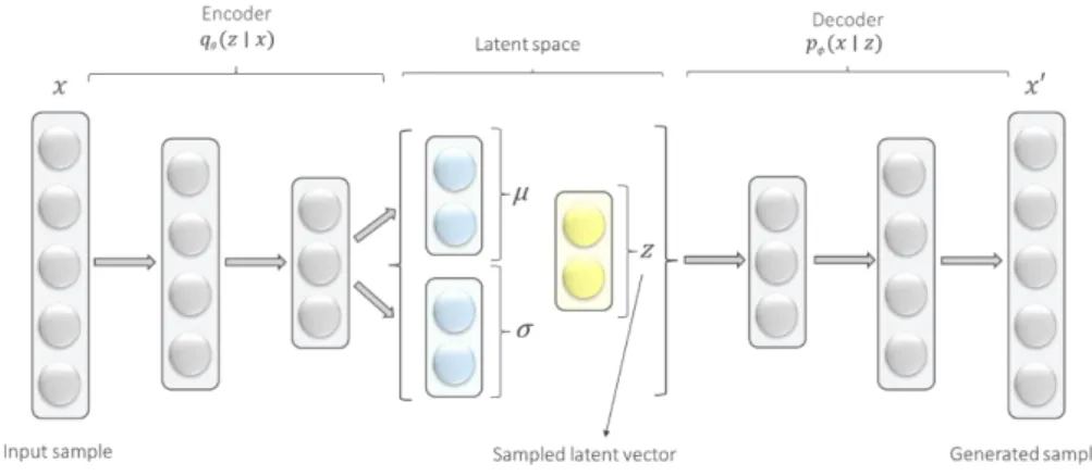
This type of autoencoders belongs to a specific class of algorithms - generative models of data (Goodfellow et al., 2016). In a very simplified form, these are the models that are trained to generate plausible looking fake samples that resemble training data. They are called autoencoders because they have constituent parts of a traditional autoencoder – encoder and decoder – however, mathematically do not have much in common with it (Doersch, 2016). A variational autoencoder (VA) is a generative model that learns a latent variable model of its input by adding constraints on the encoded representation. It was introduced as a variational Bayesian approach that involves the optimization of an approximation (Kingma & Welling, 2013) and can be trained with gradient-based methods (Rezende et al., 2014).
The encoder part of the variational autoencoder takes a sample represented by a vector 𝒙 ∈ ℝ𝒏, passes through the encoding network and produces a probability distribution in the latent
space. This distribution is Gaussian (Kingma & Welling, 2013). In practice, this is reflected in an additional variational layer consisting of a mean vector µ ∈ ℝ𝒎 and standard deviation
vector 𝝈 ∈ ℝ𝒎 of the same dimension as the latent vector. For each data sample, a point in
the latent space is sampled from the distribution and it is represented by a vector 𝒛 ∈ ℝ𝒎
which is fed into the decoder. As a result of the decoding process, a new sample is obtained, and it resembles the input sample (Figure 3.8).
29
Figure 3.8 Variational autoencoder
The generative model of the variational autoencoder is a probabilistic model and is not considered here in detail, but it is worth noting a key difference from the vanilla autoencoder that the variational autoencoder is a stochastic model where a probabilistic encoder 𝒒𝜽(𝒛 ∣
𝒙) approximates the true posterior distribution 𝒑(𝒛|𝒙), and a generative decoder 𝒑𝝓(𝒙 ∣ 𝒛)
does not rely on any particular input 𝒙. The idea is to ensure that the decoder can decode any input, and for this, one needs to define the distribution of inputs that the decoder should expect (Doersch, 2016). In literature, the variational autoencoder algorithm is referred to as variational approximation to inference (Rezende et al., 2014) which literally means prediction of latent representations given new data by approximating a posterior distribution over the latent units given the input data. Generative models are in active research and used in a wide range of interesting applications.
3.4.2 Convolutional autoencoder
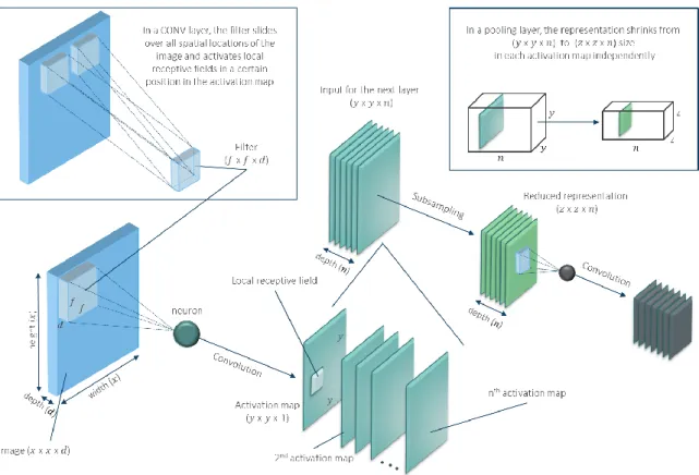
This is an autoencoder based on convolutional neural network (CNN). Convolutional architectures assume that inputs are data that has a grid-structured topology (Goodfellow et al., 2016) such as images. This allows to take advantage of the graphical object structure and encode its specific properties. CNNs were introduced by (Fukushima, 1980) under a different name, and became the basis for modern convolutional networks (LeCun et al., 1989; LeCun et al., 1998).
A CNN consists of convolutional and subsampling layers optionally followed by a fully connected layer (Figure 3.9). The convolutional process is implemented to create a feature (activity) map from the input by extracting local receptive fields across the entire image. After activation in hidden neurons, the pooling step is applied resulting in dimensionality reduction
Chapter 3
Autoencoder framework
30
of the feature map by condensing outputs of small regions of neurons into a single output. This is considered as one layer of a CNN (Ng et al., 2017).
Figure 3.9 Convolution and pooling in CNN
Each subsequent layer increases a complexity of the learned feature map. When high-level features are detected a fully connected layer is attached to the network. In supervised learning, the fully connected layer accesses the output of the previous layer and defines properties that are more related to a particular class of objects (Krizhevsky et al., 2012).
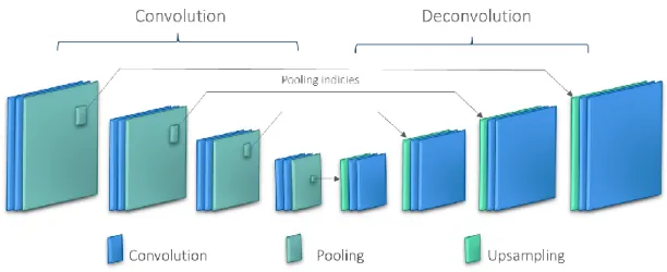
In unsupervised learning, the middle subsampling layer is connected to the decoder and proceeds with the convolutional process again to reconstruct the input image (Figure 3.10). Since training a network with the image input from scratch requires huge computational power, a convolutional autoencoder was viewed as a technique of initializing weights in a neural network (Erhan, Courville, & Vincent, 2010). It is also widely used for its conventional purpose of feature extraction (Masci et al., 2011; Du et al., 2017).
31
Figure 3.10 Convolutional autoencoder
Source: adapted from (Badrinarayanan, Kendall, & Cipolla, 2017)
3.4.3 Sequence-to-sequence autoencoder
Designed to be trained with sequential data, this autoencoder is based on another specialization of neural networks which is appropriate to handle sequences - recurrent neural network (RNN). The idea behind RNNs is to use sequential information where connections between elements form a directed circle (Jordan, 1986). There are several variants of RNNs can be found in literature: Jordan networks (Jordan, 1986), Elman networks (Elman, 1990), Bidirectional RNN (Schuster & Paliwal, 1997), Long-Short Term Memory networks (Hochreiter & Urgen Schmidhuber, 1997), Gated Recurrent Units (Chung, Gulcehre, Cho, & Bengio, 2015). The specificity of training neural networks fed with sequential data is determined by the nature of this data. A time series can be viewed as a generated sequence of values monitored over time. The unstable character of data affects the output in a way that it depends not only on the fixed input but also on how data behaved in the past. In practice, this is reflected in the loops that allow information to persist (Figure 3.11). A sequential input is processed by applying a recurrent formula (3.11) at every time step.
ℎ𝑡 = 𝑓𝑊(ℎ𝑡−1, 𝑥𝑡) (3.11)
𝑦𝑡 = 𝑊ℎ𝑦ℎ𝑡 (3.12)
where 𝒉𝒕 is a new state, 𝒇𝑾 is a function with parameters 𝑾, 𝒉𝒕−𝟏 is an old state, 𝒙𝒕 is an input vector at some time step, 𝒚𝒕 is a sequence of outputs.