Mergers and acquisitions : the case of Montepio and Finibanco

(1)

Mergers and Acquisitions: The case of Montepio and

Finibanco

Francisca Nunes Gentil-Homem Horta 152210501

Supervisor: Peter Tsvetkov

Dissertation submitted in partial fulfillment of requirements for the degree of MSc in Economics, at the Universidade Católica Portuguesa.

(2)

ii

Abstract

In August of 2010 Montepio announced its intention to purchase Finibanco. Although the purchase value and estimated synergies are known from the beginning, the process to arrive at these values is not.

The purpose of this work is to simulate the valuation process done by Montepio and, therefore, the data used is from end-year 2009. Valuation methods such as discounted cash-flows and market multiples will be used to value the two banks and it will be concluded that there are potential synergistic gains in this operation.

Given the new financial and economic data since the conclusion of the operation, the assumptions made for the future behavior of the banks’ accounts will be revised but the main conclusion will not change: even if all the parts involved in this process had been able to know that the economic crisis was going to develop into what it is today, the operation would still be considered to be profitable.

We will not arrive at a value that is close to that paid by Montepio, since we are only studying the banks of each financial group. It should be expected, however, that we arrive at smaller values than the real one, since we are considering only a part of the real operation. This is, indeed, what we will see in this work.

(3)

iii

Acknowledgments

First of all, I would like to thank my Dissertation Supervisor, Peter Tsvetkov, for his continuous orientation and availability to give feedback and advice and the patience to answer all my questions.

I would also like to thank my friends at Católica-Lisbon, especially fellow MSc in Economics and M&A seminar students for the constant help, support, advice and motivation.

Moreover, I would like to thank Montepio Geral Associação Mutualista for giving me the opportunity to do an internship in their offices and allowing me to discover and fall for the banking industry and to acquire valuable knowledge.

Finally, I would like to thank my family for giving me the opportunity and the support needed to obtain this degree.

(4)

1

1 Introduction

The purpose of this thesis is to study a potential or actual M&A operation between two companies. The two companies studied in this work are Montepio Geral and Finibanco – two Portuguese banks that were involved in an acquisition process in 2010, when Associação Mutualista – the head of Montepio Geral group – acquired Finibanco Holding, S.A. – the head of Finibanco group. In buying the entire Finibanco group, Montepio acquired all the businesses in this group, such as the bank and the insurance companies, to name a few. In this work, only the banking businesses (operating in Portugal) from each group will be studied.

I chose to do this work about an operation involving two banks because this subject would allow me to combine two areas that I am very interested in – Finance and Banking. Also, having done an internship at Montepio before the operation was finalized, I was always curious to know how such process would be developed from an inside perspective.

Although having an inside perspective will not be possible (or, if it were possible, it would not be relevant in the context of this work), a simulation of the work done at the time of the announcement of the public offer can be made. This will be the object of this work – the simulation of the valuation process of Finibanco and of its added value to Montepio. This means that most of this work will consider the present time to be December 31st of 2009, so that the data used will concern the end of the year previous to the operation. For reasons of consistency, the predictions made for future values of the banks’ accounts are based on predictions made by the International Monetary Fund (IMF) for the Portuguese economy at the end of 2009.

Obviously, being now the year of 2012, we are in a position where we are more informed about the economic conditions for approximately half of the period of our predictions, which will be 2010-14. This means that we are now aware of the sovereign debt crisis affecting Europe, and particularly Portugal, and of the new challenges faced by governments and financial institutions in the area. These new conditions and the updated predictions for the Portuguese economy made by the IMF make the predictions made for the two banks seem unrealistic and probably too optimistic.

At the face of the more recent data, the predictions made originally and the valuation model built in this work will be recalibrated in order to incorporate the new information and yield more informed and more realistic results.

In both models, besides running calculations for each bank individually, calculations of potential synergies will also be run in order to assess the potential gains generated from this operation and to calculate the price (and implied premium) Montepio would be willing to pay Finibanco to acquire its operations.

(7)

4

2 Literature Review

2.1 The Banking Sector

2.1.1 Main Drivers

The main drivers of performance in the banking sector can be divided into three main groups: strategy, execution of strategy and the environment (Harker and Zenios, 1998).

The authors highlight the main strategic decisions that have to be made by banks: product mix, which products to offer to a bank’s clients; client mix, what client profile fits a bank the best; geographical location, where the bank should operate (both internally and externally); distribution channels, which means the bank will use to sell its products.

What the bank does to achieve its strategic goals is also a set of performance drivers: x-efficiency, all technical and allocative strategies that are not scale or scope dependent; human resource management, a number of factors that influence the employee satisfaction; use of technology, amount spent on information technology; process design, the mechanism that transforms inputs into outputs.

The authors discuss three environmental factors that can influence the performance of a bank: technology, the improvements made to products in technological industries and the access customers have to information technology; consumer tastes, the change in typically preferred products.

2.1.2 Main Difficulties

Contrarily to most firms, debt is not merely a means of financing a bank, it is also its “raw material” – the money it uses to lend to clients and make a profit from the gap in interest rates. Therefore, defining debt and capital in a financial service company is a less straightforward process than for other types of businesses. Also, it is very hard to calculate the reinvestment needs: in the calculation of net capital expenditures, the main difficulty is that investment for growth is often categorized as operating expenses and capital expenses tend to be close to zero and, consequently, so does depreciation; in the calculation of working capital, defined as the difference between current assets and current liabilities, the main problem is that these numbers may change a lot and these changes may be unrelated to reinvestment for growth (Damodaran, 2009).

The fact that it is extremely hard to measure reinvestment for banks has two important consequences: we cannot estimate cash flows without estimating reinvestment; and it is harder to estimate an expected growth rate for the future without a reinvestment rate. Damodaran (2009) suggests two alternative

(8)

5 calculations for bank cash flows: earnings as cash flows, discount earnings to the present to calculate the value of a bank; pseudo cash flows, use an alternative/adaptation to the standard definition of cash flows.

2.2 Valuation Methods

As was discussed above, it is extremely hard to measure the level of debt of a bank. Consequently, it is equally hard to calculate the value of a bank using valuation methods that have the level of debt as an input.

2.2.1 Discounted Cash Flows (DCF) Models

It is generally accepted that the DCF is the method to use when valuing a firm. The inherent mindset is fairly easy to understand and the necessary calculations are quite simple, once the estimations for the cash flows and discount rate have been done. The DCF method considers that the value of a company is the present value of the sum of all its (expected) future cash flows. The present value is obtained by discounting each cash flow at a rate that accounts both for the risk implied in these cash flows and for the time value of money.

∑ [ ] ( )

Where: n = Life of the firm

E[CFt] = Expected cash flow in period t

i = Discount rate that reflects the uncertainty of the expected cash flows

As stated by Holt et al. (1999), the inputs needed for a DCF analysis are the cost of capital, the levels of free cash flows and investment and free cash flow growth.

The most common procedure is to discount cash flows to the cost of capital, which is usually computed with the weighted average cost of capital (WACC) formula:

( )

Where: D is the value of debt E is the value of equity

(9)

6 As can be seen in the formula, in order to use this method one needs to know the amount of debt of a firm, which can be quite hard in the case of a bank, as discussed previously. In this work, the valuation methods used are meant to value only the equity of banks.

2.2.1.1 Discounted Cash Flows to Equity

In this case, the cash flows that are discounted are the expected cash flows to equity, i.e., “the residual cashflows after meeting all expenses, reinvestment needs, tax obligations and net debt payments (interest, principal payments and new debt issuance)” (Damodaran, 2002). These cash flows are discounted at the appropriate discount rate – the cost of equity, “i.e., the rate of return required by equity investors in the firm” (Damodaran, 2002).

∑ [ ] ( )

Where: n = Life of the firm

E[CFt] = Expected cash flow to equity in period t ke = Cost of equity

If, instead of discounting the cash flows calculated as discussed above, we decide to discount future dividends we are in the presence of the special case of the DCF model applied to equity valuation – Dividend Discount Model (DDM), which “requires estimates of dividend growth and the level of dividends and earnings” (Holt et al., 1999). Damodaran (2009) ends up concluding that this is the best adaptation of the DCF method to calculate the value of a bank and discusses some ways of increasing the quality of the obtained estimation.

The first is the cost of equity used to discount the dividends. Damodaran (2009) advises the use of bottom-up betas, both due to the noise implicit in regression betas and to the fact that there are many public firms in the financial sector, which should make the estimation of bottom-up betas easier.

The second piece of advice is that one should not adjust for financial leverage (unlever and then relever betas) for financial service firms for two reasons: the capital structure of these firms is usually quite similar and, as discussed before, debt is very hard to measure for this firms. This will mean that the average levered beta for comparable firms will be used to value the firm as the bottom-up beta.

(10)

7 This conclusion about the bottom-up beta leads us to the next suggestion given by the author: we should define narrower sectors when calculating the average levered beta, inside the financial service sector, so that we do not end up using the same levered beta for every firm in the sector.

The fourth recommendation is that betas are adjusted according to the stage of life in which the firm is. This means that high growth firms (usually younger) should have higher betas, and therefore higher costs of equity, than more mature firms.

Copeland et al. (2000) recommend an alternative way to value a bank. The authors recommend that one should forecast free cash flow to equity (FCFE) and discount it at the cost of equity. The cash flow to equity is the cash flow left over for equity investors after debt payments have been made and reinvestment needs met1 (Damodaran, 2009).

The difficult task is, now, to measure reinvestment. For banks, this reinvestment is made in regulatory capital, i.e., banks invest in capital to meet the limits imposed by the regulatory authorities.

2.2.1.1.1 Cost of Equity

The Capital Asset Pricing Model (CAPM) was first introduced in the mid-1960s by John Lintner, William Sharpe and Jack Treynor as an answer to the question of what the expected return on an asset whose beta is neither 0 nor 1 should be (Allen et al., 2008).

The CAPM lies on some assumptions that are important to mention: there are no transaction costs, all assets are traded, investments are infinitely divisible, everyone has access to the same information and, consequently, it is impossible to find under or overvalued assets in the market (Damodaran, 2002).

Risk-free Rate

An important idea of the CAPM is the existence of a risk-free asset, which has a risk-free return. This asset will be used by investors to make combinations of the market portfolio with the risk-free asset in a way that it will reflect their degree of risk aversion, since it is assumed that they can borrow and lend at the same rate of interest (Allen et al., 2008). This means that investors will borrow at the risk-free rate to invest more in the market portfolio if they are risk lovers or hold a big proportion of the risk-free asset if they are risk averse.

1

(11)

8 The importance of the risk-free rate for the CAPM justifies that we are very careful when choosing which asset to consider as risk-free. Damodaran (2002) defines three conditions that are needed to make such a choice: the returns on this asset must be known with certainty; the asset must not carry any default risk (usually, this condition should exclude all securities issued by private firms and leave only those issued by the government); there can be no reinvestment risk (there cannot be the risk of not knowing at which rate to reinvest, once the investment matures).

Allen et al. (2008) highlight that, since the CAPM works period by period then the risk-free should be short-term. However, the rationale behind the CAPM was built with the basic idea that investors demand a premium on the risk-free rate for holding some asset that is risky. Therefore, the authors end up concluding that one can use a long-term risk-free rate as long as the market returns used to calculate the market premium are long-term as well. Damodaran (2002) adds to this and stresses that, when calculating the market premium, one must use the return from the asset that has been considered as risk-free when the risk-free rate was chosen, i.e., the two risk-free rates must be the same.

In this work, the arithmetic average of the daily returns of the index of Generic German bonds, with maturity of 10 years2, for the period 24/02/1997-31/12/2009 will be used, since this is the period for which there is data on the index of Generic Portuguese bonds3, with maturity of 10 years (which will be used to calculate the country risk premium).

Beta

The discussion around the investors choosing a combination of the market portfolio and the risk-free asset leads to the discussion of the level of risk of an individual asset. “The risk to an investor of an individual asset will be the risk that this asset adds on to the market portfolio” (Damodaran, 2002), i.e., if the returns of an asset are somehow correlated with the returns of the market portfolio, that asset has more market risk than firm-specific risk, which is harder to diversify away. One good measure of risk is the beta of an asset:

From this formula, it can be seen that the beta of the market portfolio will be 1 (covariance of the market with itself is the variance, which then cancels out). Furthermore, assets that are riskier than the market

2_{Bloomberg Ticker: GDBR10 Index.} 3

Bloomberg Ticker: GSPT10YR Index

4

3

(12)

9 portfolio will have betas greater than 1 and assets that are less risky will have betas lower than 1 (particularly, the beta of the risk-free asset is 0) (Damodaran, 2002).

In order to obtain an expected rate of return from this model, one must first estimate a value for the beta. Damodaran (2002) suggests three different methods: historical data; accounting data; and fundamental characteristics.

The method of using historical data consists of running an ordinary least squares (OLS) regression of past individual returns on past market returns. The beta will then be the estimated value obtained for the slope.

This method, however simple and practical it may seem, has some weaknesses that are worth mentioning: the standard errors, i.e., the fact that no regressions are perfect and all come with errors and that, in order to obtain “true” estimates, one has to compute interval estimates, which at a good confidence level can become quite wide; the possible failures of the local indices; and the incapacity of the regressions to reflect changes in the financing mix of a firm.

The method of accounting data estimates the betas by relating the accounting earnings of a firm with those of the market. Although this method seems rather intuitive, it has three important drawbacks: accounting betas will be biased down relatively to market betas, due to the smoothed expenses and revenues; accounting earnings are influenced by non-operating factors; and accounting earnings are measured less frequently, which may result in a sample that is smaller than desirable (Damodaran, 2002).

The method of using fundamental characteristics of the firm is extremely useful for companies for which historical prices cannot be obtained, and therefore betas based on historical data cannot be estimated. Both Damodaran (2002) and Allen et al. (2008) discuss on factors that are relevant to estimate the beta with this method: cyclicality, i.e., whether or not the outcome of a firm depends on the state of the business cycle (the more it does, the highest the beta should be); the operating leverage of the firm (measured as the ratio of fixed costs over total costs or as the ratio of fixed costs over variable costs), which, in the case of being high, suggests higher variability in the net income, thus higher risk and, therefore, a higher beta; the type of product sold by the firm (luxury goods should indicate a higher beta than necessary goods); the financial leverage of the firm (a higher level of financial leverage means that, due to the increased interest payments, the variability of the net income will also be higher, increasing the level of risk and, therefore, the beta).We can see this in the formula that relates the unlevered beta, i.e., the beta the company would have if it were all-equity and the levered beta:

(13)

10 Where: βL = Levered beta for equity in the firm

βu = Unlevered beta of the firm t = corporate tax rate

= Debt/Equity Ratio

In this work, historical betas will be used. The simple average market beta for the Portuguese banking industry (excluding Finibanco) for the period 24/02/1997-21/12/2009 was computed. This beta is used for both banks for the following reasons: for Finibanco, there was not enough data on share’s prices to compute a reliable beta and for Montepio there is no data at all, since it is not a public bank.

Market Risk Premium

While the beta of an asset measures how much risk that asset adds on to a market portfolio, the risk premium is the extra return demanded by an investor to invest in that asset instead of investing in the risk-free asset. Although this is quite simple to describe, measuring the market risk premium is not an easy task. Below, some methods used for this calculation are discussed. Damodaran (2002) and Copeland, Koller and Murrin (2000) divide the most common methods into two groups: historical data and ex ante estimations.

Damodaran (2002) highlights the three decisions that have to be made before using historical data to estimate a market risk premium: the time period used; the risk-free security; and the averaging method (arithmetic or geometric averages). Copeland et al. (2000) make recommendations on each of these decisions: it is better to use longer time frames, so that there are both cycles and counter cycles in the sample; the risk-free security that carries the least amount of problems (however technical they may be) is the 10-year Treasury bond; the geometric average is the most correct method to measure historical performance but the arithmetic average is more forward looking and this is the one that should be used; also, it is recommended that a survivorship bias of 1,5% to 2% is subtracted from the historical arithmetic average.

Damodaran (2002) stresses that measuring the market risk premium for a country other than the US can be difficult and yield useless results. Thus, the author presents three methods to calculate the country risk premium that will then be added to the base premium for equity risk. The first method measures country risk premium with a default spread on bonds issued by the country and introduces it additively in the

(14)

11 calculation of the cost of equity4. The second method measures the equity risk premium in a country by comparing the standard deviations of stock prices in that country and in the US5. Finally, the last method measures a country risk premium using both the country default spread and the relative standard deviation of the equity market of that country in relation to that of the bond market of that same country6.

In what concerns the other group of methods – ex ante estimates – both Damodaran (2002) and Copeland et al. (2000) discuss a few alternatives. The first alternative is what Damodaran (2002) calls the implied equity premium, which is obtained from the current value of a company and from the expectations for future dividends and growth rate7. The second one computes the equity discount rate as an internal rate of return, using the current book value of the firm and stock price and expectations for future ROE and book value8. Copeland et al. (2000) conclude that they prefer not to use ex ante estimations.

In this work, a risk premium computed as the difference between the arithmetic averages of the daily returns of the PSI20 index (annualized) and the GDBR10 index, for the period 24/02/1997-31/12/2009 will be used. Also, a survivorship bias of 1.5% is subtracted to the value obtained and a country risk premium (measured with the third method discussed by Damodaran (2002) described above) is added.

Following the discussion on the fact that investors hold the market portfolio and the risk-free asset, one arrives at the conclusion that the expected return on an asset is linearly related with its beta (Damodaran, 2002):

[ ] ( [ ] )

Where: [ ] = Expected Return on asset i

= Return on the risk-free asset (risk-free rate) = Beta of asset i

[ ] = Return on the market portfolio

4 5 6 7 [ ] [ ] 8 _∑ [( ) ] ( )

(15)

12

2.2.1.1.2 Cash Flows

Damodaran (1994) describes three approaches to estimate future cash flows: expected value, which represents the single best estimate of the cash flow in a single period, since it incorporates all possible good and bad outcomes; scenario analysis, in which cash flows are estimated under different scenarios and conclusions are presented in the form of a range of values instead of a single value; and simulations, in which distributions of values are estimated for each parameter in the valuation and simulations are made by drawing outcomes for each distribution to derive a distribution for the value of the business. As stated by Holt et al. (1999), it is usual to make annual forecasts for the first three to ten years and consider that profits, returns and discount rates will remain constant after that (or grow at a constant growth rate).

It is also important to discuss the notion of terminal value, since it will usually represent a significant proportion of the total present value of a firm (Froot, Kester and Molley, 1997). Damodaran (1994) describes three ways to estimate the terminal value of a firm: to assume a liquidation of the firm’s assets and estimate how much would be paid for them; to assume that the firm is not liquidated and apply a market multiple to estimate the value of the firm; to assume that the firm is not liquidated and that it will continue to grow at a constant growth rate.

2.2.1.1.3 Growth Rate

Damodaran (1994 and 2000) presents three basic ways to estimate growth: historical growth rate; outside estimates of growth; and fundamental determinants of growth.

In order to use historical data to estimate a growth rate, two important decisions have to be made: whether to use arithmetic or geometric averages and whether to use revenues or earnings growth. The author gives an insight for each decision: “the geometric average is a much more accurate measure of true growth in past earnings” (Damodaran, 2000) and “historical growth in revenues is a far more useful number when it comes to forecasting than historical growth in earnings” (Damodaran, 2000), since “revenue growth tends to be more persistent and predictable than earnings growth” (Damodaran, 1994).

When it comes to outside estimates of growth, the author discusses two sources of estimates: management estimates and analyst estimates. Management estimates have the advantage of being simple to obtain since the numbers are provided by the managers; and the possible dangers of obtaining biased prospects for the future and of using a combination of inconsistent assumptions. Analysts, on the other hand, have access to more information besides historical data, which can potentially increase the quality of their predictions: firm-specific information that has been made public since the last earnings report;

(16)

macro-13 economic information that may impact future growth; information revealed by competitors on future prospects; private information about the firm; and public information other than earnings (Damodaran, 1994 and 2000). The author concludes that analysts provide better short-term forecasts of earnings than models that depend purely upon historical data but this superiority is surprisingly small for long-term forecasts.

The fundamental determinants of growth depend on which variable is being used. If the goal is to estimate growth in earnings per share then the fundamentals are the return on equity and the retention ratios. If the goal is to estimate growth in net income, the fundamentals are return on equity and the equity reinvestment rate. Finally, if the goal is to estimate the growth in operating income, three different scenarios have to be considered: the scenario of stable return on capital, where the expected growth of the EBIT is simply the product of the reinvestment rate by the return on capital9; the scenario of positive and changing return on capital, where the computation of the expected growth rate is very similar to the one of the first scenario but adds the variation of the return on capital10; the scenario of negative return on capital, in which case following steps must be followed: project growth in revenues, estimate the operating income and estimate reinvestment needs that allow for generating revenue growth.

2.2.1.2 The Adjusted Present Value (APV)

The Adjusted Present Value (APV) Model is also a DCF model. Contrarily to what was previously described about the WACC, the APV intends to be a versatile and reliable managerial tool (Luehrman, 1997a) and does not attempt to catch the effects of financing in an adjusted discount rate (Allen et al., 2008). The APV is able to provide a breakdown of all value-creating components, value them separately and discount each one at the rate that best represents its level of risk. The present value of a company will then be the sum of all these present values.

Where: base-case NPV = the value of the firm without any investment project or debt financing

Possible financing side effects: interest tax shields (positive); issue costs of debt (negative); subsidies from the government or a supplier (positive)

9 Where: _{( )} ( ) 10

(17)

14

2.2.2 Returns-based Valuation

This type of valuation methods focuses on the returns of a firm, rather than on its earnings, dividends or growth rates. With this type of models, the value of a firm is the sum of capital invested currently in the firm and the present value of excess returns that the firm expects to make in the future (Damodaran, 2009).

According to Damodaran (2009), the two fundamental inputs of this approach are: equity capital invested currently in the firm and expected excess returns to equity investors in the future. Usually, the book value of equity is a good enough approximation of the value of equity capital invested in a firm, since most assets in financial service firms will be marked to market and the amounts of depreciation are negligible for these firms. The excess returns will be measured as:

( ) ( )

The excess returns are then discounted back to the present at the cost of equity and added to the current capital equity invested in the bank to obtain the current value of the equity bank.

2.2.3 Asset-based Valuation

Typically, in asset-based valuation, the existing assets of a firm are valued net of debt and other outstanding claims to obtain the value of equity. However, due to what was discussed about the difficulty of defining and measuring the value of debt of a financial service firm, it works in a slightly different way to value banks.

For a bank, measuring the value of assets means mostly that we have to measure the value of its loan portfolio. Damodaran (2009) suggests that this valuation be based on expected cash flows. The discount rate should be obtained either through the rating given by a ratings agency or by measuring the default risk of the portfolio. Then, in order to obtain the value of equity, we need to subtract the value of deposits, debt and other claims on the bank to the value we obtained for assets.

2.2.4 The Method of Multiples

As Kaplan and Ruback (1996) explain: “in these methods, a ratio or multiple of value relative to a performance measure is calculated for a set of guideline or comparable firms”. Examples of performance measures are earnings before interest, tax, depreciation and amortization (EBITDA), earnings before

(18)

15 interest and tax (EBIT), net income or revenue. These performance measures can be used either with their current values or with expectations for the future, forming then the leading multiples. In fact, Goedhart, Koller and Wessels (2005) point out that “both the principles of valuation and the empirical evidence lead us to recommend that multiples be based on forecast rather than historical profits”.

The market value of a company is obtained by multiplying the market multiple by the performance measure of that same company.

It is important to mention the two assumptions on which this method is built: it is assumed that the future cash flows of the company that is being valued and of the companies considered to calculate the market multiple grow at the same rate and have the same level of risk; also, it is assumed that the value of the company varies in direct proportion with the performance measure being used (Kaplan and Ruback, 1996).

In sum, what sets this method apart from the DCF methods discussed above is that, while valuations done by discounting cash flows are based upon expectations and estimates for that one company, those that are done with multiples reflect essentially market expectations for the future for that particular sector or industry.

Similarly to what happened with the DCF methods to value financial service firms, this work will focus mostly on multiples that allow for an estimation of the value of equity. For this purpose, Damodaran (2009) discusses the price earnings and the price to book value ratios.

Both ratios are used for financial service firms in the same way as for any other firm:

2.2.5 The DuPont System

The DuPont system is a useful tool for ratio analysis of a firm, since it breaks down the return on assets (ROA) and the return on equity (ROE) (Allen et al., 2008). However, it is also used to value the equity of a bank, assuming that value is generated by the net asset value (NAV):

(19)

16 ROEForecasted = ROA x Equity Multiplier

Equity Multiplier is the maximum leverage allowed (12.5 for Tier I 8%) ROA = Asset Utilization (or Turnover) x Profit Margin =

( )

2.3 Mergers and Acquisitions

There are many reasons why companies acquire other companies and, although most of them are probably good, Roche (2002) and Ficery et al. (2007) give some advice that should be kept in mind by companies that are considering making an acquisition: companies should do what they know best and not try to learn a new business without the time, the energy and the money needed to make a few mistakes; the M&A strategy should be an integral part of the business plan of the company; synergy expectations that cannot be translated into dollar (or some other currency) amounts should not be included in synergy calculations.

2.3.1 Main Drivers of M&A

Much has been said and written about what drives M&A operations. The main drivers of M&A activity have changed over time: in the period 1894-1904, M&A activity was mainly driven by economic turbulence; in the period 1890-1930, M&A operations were related with the diffusion of electricity and the internal combustion engine; in the period 1971-2001, the main driver became the diffusion of information technology, with the additional drivers of advances in information technology and innovations in organizational design and fundamental economic shocks, such as deregulation, technological innovation, demographic shifts and input price shocks also having some relevance in operations occurring in the 1980s (Bruner, 2004).

The author stresses that the success of a deal depends largely on its context and, therefore, discusses the drivers of M&A profitability on a local basis. The author defines four different cross-sections (strategy, investment opportunity, deal design and governance) and discusses the drivers within each cross-section.

The main drivers within the strategy cross-section are: focus vs. diversification (the purpose of a specific M&A operation); strategic restructuring (selling or redeploying underperforming businesses); the initiation of M&A programs (an M&A operation is the first step towards a series of acquisitions); strategic synergies

(20)

17 (the main motivation for an acquisition is to take advantage of some kind of synergy); grabs for market power (market share and returns to shareholders are closely related).

When it comes to the cross-section of investment opportunity, the author highlights the following drivers: targets that can be restructured (i.e., whose profitability can be improved); privately owned assets (on average, private firms are cheaper than public firms); crossing borders (premiums paid are higher for foreign target firms).

In the case of the deal design cross-section, the author gives emphasis to the following drivers: form of payment: cash vs. stock (already discussed above); Leveraged Buyouts (shareholders of target firms involved in LBOs earn large abnormal returns); use of earnouts (bidder firms earn higher returns if the payment is contingent on future performance); use of collars (another risk management device that changes the payment in the case of pre-determined triggers in the buyer’s price).

Finally, the main governance drivers are: activism by institutional investors (the ability that institutional investors have to block mergers); what managers have at stake (how much of the acquiring company is owned by its managers); friendly vs. hostile approach to the target (studies show that tender offers earn higher abnormal returns than friendly negotiated transactions); use of anti-takeover defenses (defenses enhance the bargaining power of the target firm).

Houston, James and Ryngaert (2001) discuss drivers of merger profitability in the banking sector. The authors find that the most relevant sources of gains are cost cuts resulting from the elimination of overlapping operations and the consolidation of backroom operations. The authors also find that market overlap transactions yield significantly higher returns than those of market expansion transactions. The authors measure market overlapping with the following formula:

∑ ( )

∑ ,

Where: n is the total number of cities in which either bank has an office

Ti and Bi are the total number of offices the target and the bidder (respectively) have in city i

This measure of overlap takes a maximum of 0.5 when there is complete overlap and a minimum of 0 when there is no overlap.

(21)

18

2.3.2 Synergies

2.3.2.1 Types of Synergies

Damodaran (2005) defines synergy as “the additional value that is generated by combining two firms, creating opportunities that would not [have] been available to these firms operating independently”. The author categorizes synergies into two groups: operating synergies (those synergies that affect the operations of the combined firm; they can take the form of economies of scale, greater price power, combination of different functional strengths and higher growth in new or existing markets) and financial synergies (include tax benefits, diversification, a higher debt capacity and uses for excess cash).

2.3.2.2 Valuing Synergy

Valuing synergy can be a troublesome and uncertain process. However, it is still an important step in the valuation of a prospect acquisition/merger. In this section, we will present some methods that can be used to value synergy.

Damodaran (2005) presents the two fundamental questions for the valuation of an operating synergy: “What form is the synergy expected to take?” and “When will the synergy start affecting cash flows?”. The author suggests that this valuation is done in three steps: firstly, we value each company separately; secondly, we value the combined company without taking synergies into account; finally, we value the combined company with the effect of the synergy and obtain the value of the synergy by taking the difference between the two values obtained for the combined firm.

In order to obtain an accurate valuation of financial synergies, Damodaran (2005) suggests that we divide them into three groups: a greater “tax benefit” (i.e., tax shields); an increased debt capacity; a better use for “excess” cash. In the case of greater “tax benefit”, the value of the synergy is the present value of the savings in tax expenses that is due to the merger. In the case of increased debt capacity, the author mentions a few models that have been developed to analyze this type of financial synergy from different perspectives – reduced default risk; reduced debt to equity choices and limited liabilities; and option pricing applied to higher debt capacity. In the case of “excess” cash, one simple way to value the synergy is to compute the value of the projects that would have been rejected if it were not for the merger.

(22)

19 Using Earnings-Based Financial Information to Value Synergies

Sahni and Sirower (2006) present an alternative model to value synergies that yield combinations of cost reductions and revenue enhancements.

If we are in the case of cost reductions alone, we can measure the improvements that need to be made to compensate for the premium paid (measured as a percentage of the pre-acquisition addressable operating cost base of the target) with the formula:

Where: %P is the premium paid for the target company Π is the pretax profit margin

If, on the other hand, we are in the case of both cost and revenue synergies, we can measure the required cost reductions after taking account of the benefits of the expected percentage revenue synergies (%SynR) with the formula:

( ) ( ) ( )

Where: %P is the premium paid for the target company R is the revenue

Π is the pretax profit margin

After calculating the percentage required cost and revenue improvements necessary for a given premium, one has to assess whether the obtained values are plausible.

2.3.2.3 Sharing Synergy Gains

Assuming that synergies can create value in an acquisition, one should then discuss how to share these gains between the bidder and the target firms of the operation. The fairest way to share synergies seems to be to do it in a way that the firms get the synergy gains in proportion to their contribution to these same gains (Damodaran, 2005).

(23)

20

2.3.2.4 Evidence on Synergies

Damodaran (2005) discusses two methods to evaluate the true existence of synergies in a given operation.

The first one is to measure the individual market values of the firms involved in an operation (before the announcement of the deal), sum them up and compare the resulting value with the market value of the resulting firm, after the announcement of the deal. One can consider that there was a synergy if the value of the resulting firm is greater than the sum of the values of the two individual firms. Bradley, Desai and Kim (1988) show evidence that the value of the combined firm increases 7.48% on average. However, the authors stress that this can be due to many factors besides synergistic gains.

The other method is to evaluate whether the resulting firm is more profitable or grows at a faster rate than the firms operating separately. Lehn and Mitchell (1990) show that a surprising number of acquisitions (20.2% of the acquisitions made in the period 1982-1986) were sold off a few years later.

According to Damodaran (2005), evidence shows that the shareholders of target firms are the clear winners in takeovers. Actually, Jensen and Ruback (1983) concluded (from reviewing 13 studies) that target shareholders make an average return of 20%-30% around the time of the operation. Additionally, Sahni and Sirower (2006) conclude that, on average, acquirers underperform their industry peers. On the other hand, the authors stress that 35% to 40% of the deals studied benefit the acquiring firm. The authors also conclude that merger operations create value at the macroeconomic level, i.e., even though these operations tend to harm the acquiring firms and benefit the target firms, in the aggregate there is value creation of 1% at the announcement.

2.3.2.5 Most Common Errors

Damodaran (2005) discusses the most common sources of error in valuing synergies: subsidizing target firm stockholders, i.e., overpaying target firm stockholders for synergies that were not created by them; using a wrong discount rate, i.e., the right discount rate to use is the cost of equity of the combined firm; and mixing control and synergy, i.e., not distinguishing between value created by better control skills and value created by synergies, which may possibly lead to using the wrong discount rate.

Ficery, Herd and Pursche (2007) discuss common errors in capturing synergistic gains: defining synergies too narrowly or too broadly; missing the window of opportunity; incorrect or insufficient use of incentives; not having the correct people involved in synergy capture; mismatch between culture and systems; and using the wrong process.

(24)

21

2.3.3 Forms of Payment

The two most common forms of payment in an M&A operation are stock and cash (paying in cash often implies raising debt or issuing shares). Roche (2002) stresses that for a private firm it may not be a choice to buy another firm with shares, since they are not marketable. Zhang (2001)adds to this and highlights four other factors that the author proves to be relevant in segregating cash financing from share financing: stock market performance of the acquirer (the better the performance of the acquirer’s share on the stock market, the more preferable is the choice of stock financing); return on equity of the acquirer (the higher the return on equity of the acquirer, the more preferable it is to choose cash financing); relative size of the target to the acquirer (the larger is the size of the target, the more stock financing will be chosen, since there will not be enough cash to finance the operation); and the ratio of the acquiring firm’s dividend payout (the higher the dividend payout of the acquirer, the more preferable is the choice of cash financing).

Travlos (1987) studies the returns of the stocks of the bidding firm around the time of the announcement of the operation and concludes that acquiring firms suffer significant losses in pure stock exchange acquisitions but experience “normal” returns in cash offers. These results seem to be consistent with the signaling hypothesis, which says that financing a takeover operation with stock signals that the stock is overvalued. Sahni and Sirower (2006) draw the same conclusion that cash deals “markedly outperform stock deals”. Additionally, the authors conclude that one year later, the gap of performances between the two types of financing doubled.

(25)

22

3 Industry Review

The two companies studied in this work are part of the Portuguese banking sector and this is the only geography in which they operate so this market shall be the focus of our analysis in this section.

The banking sector in Portugal is characterized by having many small players but only a few large players – in 2009, the five biggest banks (Caixa Geral de Depósitos, Banco Comercial Português, Banco Espírito Santo, Banco BPI and Santander Totta) represented almost 80% of the total assets of the sector11. In fact, we can use the total value of assets of each bank to divide them into four groups: the three biggest banks (CGD, BCP and BES), with individual total assets larger than €80 billion; two medium banks (Santander Totta and BPI), with individual total assets between €45 billion and €49 billion; five medium-small banks (Montepio, Barclays, Banif, Crédito Agrícola and Banco Popular) with individual total assets between €10 billion and €19 billion; and a group of smaller banks with individual total assets below €8 billion.

3.1 Macroeconomic and Financial Setting

Since the summer of 2007, the modern world has been experiencing adverse financial market conditions and a less favorable macroeconomic situation. 2009 was the first year (for which there is significant data) in which there was a reduction of the global economy. For instance, in Portugal, the Gross Domestic Product (GDP) decreased by 2.7%. Also, the Portuguese budget deficit was 9.3% of the GDP and the unemployment was greater than 10%.

Also, between 2007 and 2009, all modern countries experienced higher credit needs, which increased the volatility levels and led to the downgrading of the public debt ratings of some of these countries. These downgrades, in turn, led to the downgrading of the debt of many private firms in these countries, increasing both the cost of issuing debt and the difficulty of placing this debt in the market.

These economic and financial conditions have consequences for the activity of companies in Portugal, namely that of banks, which will be analyzed for each of the banks studied in this work.

3.2 Expected Future Trends

The main challenges for banks in the future years go from areas such as the commercial banking income growth to the deterioration of asset quality indicators to the already discussed solvency requirements.

11

(26)

23 BES (2010) presents three main reasons for why banks should be concerned with the growth in banking income: increased cost of funding; historically low interest rates; and increased deposit competition. Deloitte (2010a) believes that a good solution to this problem may be seeking growth in weak markets. Also, Deloitte (2010b) stresses that, in trying to find new sources of revenue, one big challenge will be trying not to copy what the other banks are doing. Gordon and Lacy (2011) highlight that bank switching almost doubled since the financial crisis, when compared to pre-crisis numbers. This means that bank clients are nowadays more willing to change banks and that banks will have to fight harder to maintain longer relationships with their customers. The authors believe this should be done by improving the quality, the transparency and the honesty of the service offered.

In terms of the deterioration of asset quality indicators, both BES (2010) and Deloitte (2010a) show concerns with the bad performance of loans, especially with commercial real estate loans. Another concern in this area, which can be seen as a possible consequence of the first one, is the deterioration of coverage ratios globally.

Finally, another source of concern, which has been briefly discussed above, is capital management. Not only are banks uncertain about future regulatory changes and how they may impact their spreadsheets (Deloitte, 2010a) but they are also afraid of less favorable scenarios (due, for instance, to the current crisis in the Euro are) and may feel the need to raise capital. In order to best meet the complex demands of future regulation, Culp and Markson (2012) believe that the framework for regulatory response should be closely tied to the bank’s overall strategy.

3.3 Regulation

The following entities have major regulatory roles in Portugal: Banco de Portugal (the central bank of the Portuguese Republic); the Portuguese Securities Market Commission (also known by CMVM, the initials for its Portuguese name); and the Portuguese Competition Authority.

3.3.1 Banco de Portugal

The main objective of the Bank (since the establishment of the European Community) is to maintain price stability. However, it performs another task that is quite relevant for this work, included in the Prudential Supervision function: the Bank, similarly to the European Commission directives on financial activity, sets limits on the amounts of own funds an institution may hold: “own funds shall never be lower than

(27)

24 minimum equity capital, and at least 10% of net profits in each fiscal year shall be allocated to the building-up of legal reserves building-up to the amount of equity capital” (Banco de Portugal website). The details of these calculations are discussed under the subject “Basel”.

Basel

In 1988, the Basel Committee on Banking Supervision (one of the standing committees located at the Bank for International Settlements (BIS)) introduced a measurement system, which intended to prepare for “the implementation of a credit risk measurement framework with a minimum capital standard of 8% by end-1992” (BIS website). This system is commonly referred to as the Basel Capital Accord and has been subject to some revisions since. The current prudential framework is known by “Basel II” and is the result of the revision that started in 1999.

Basel II is structured into three areas (pillars): calculation of minimum capital requirements, supervisory review process and market discipline.

The first pillar “sets out the rules for the calculation of the minimum capital requirements for credit, market, […] operational risk” (Banco de Portugal) and, in some cases, the counterparty credit risk. The second pillar “combines a set of principles essentially intended to reinforce the linkage between internal capital held by institutions and the risks arising from their businesses” (Banco de Portugal). It completes the first pillar by including not only those risks that were not totally captured in pillar 1 but also those not included in pillar 1 at all. The third pillar “aims to promote disclosure of information by institutions, in different markets in a sufficient, consistent and transparent manner in order to ensure effective market discipline” (Banco de Portugal).

As mentioned before, the current prudential framework is what is called the “Basel II”. However, there have been efforts to improve it and to form what is already known as “Basel III”. Although this does not impact the activity of the banking system yet, it surely plays a role in the forecasting of the future. Therefore, we shall also discuss this accord as something that the two players in this work (especially Montepio) had in mind during the acquisition (and merger) process.

The new reforms aim to “raise the resilience of individual banking institutions to periods of stress” and to diminish “risks that can build up across the banking sector as well as the procyclical amplification of these risks over time” (BIS website).

(28)

25

3.3.2 CMVM

The Portuguese Securities Market Commission has “the task of supervising and regulating securities and other financial instruments markets (traditionally known as “stock markets”), as well as the activity of all those who operate within said markets” (CMVM website).

3.3.3 The Portuguese Competition Authority

“The [Portuguese] Competition Authority’s mission is to ensure compliance with the competition rules in Portugal” (website). In what concerns this work, the most important power that the Authority has is to “decide on mergers and acquisitions”. According to the Regulation No 120/2009 of March 17th 2009 - Notification Form for Concentrations between Undertakings, the parties involved in a concentration between undertakings12 must provide all the information necessary for the Authority to be able to decide on the operation in the most accurate way possible. This is done through a Notification Form that is presented to the Authority prior to the operation.

12_{This obligation is in order if “Their implementation creates or reinforces a share exceeding 30% of the national}

market for a particular good or service or for a substantial part of it” or “In the preceding financial year, the group of undertakings taking part in the concentration have recorded in Portugal a turnover exceeding EUR 150 million, net of directly related taxes, provided that the individual turnover in Portugal of at least two of these undertakings exceeds two million euros.” (Law No 18/2003, June 11th, Article 9).

(29)

26

4 Companies Review

4.1 Montepio Geral

In the context of this work, it is relevant to discuss both Associação Mutualista (the head and owner of the group) and Montepio Geral (the bank).

Associação Mutualista (AM) is the head of the largest mutual and social economy group in Portugal. It was created in 1840 with the goal of acting as a complement to the Portuguese Social Security system in the protection of its associates. Caixa Económica (CEMG) was created a few years later as an additional provider of financial services, since AM is mainly characterized by its supply of savings products.

AM has no shareholders and its “owners” are the members. It is to these members that the earnings are distributed each year, in proportion to the amount held by the member in each subscription. CEMG, on the other hand, works pretty much as any other bank, paying dividends and/or receiving an endowment to increase its institutional capital at the end of each year.

4.1.1 Competitors

As mentioned in section 3, given its size, Montepio’s most direct competitors are those of the above-called group of medium banks: Barclays, Banif, Crédito Agrícola and Banco Popular.

Barclays is an English financial group founded in 1690. The group started an expansion process in the beginning of the 20th century and it began operating in Portugal in 1985.

Banif (Banco Internacional do Funchal) was created in 1988 in Madeira, with the total assets and debt of the extinct Caixa Económica do Funchal.

Crédito Agrícola was founded in 1911, although the concept of co-operative financial groups already existed since the 15th century. The values and mission promoted by Crédito Agrícola are very similar to those of Montepio. However, it works in a slightly different way: each branch (Caixa) is autonomous but works under the orientation and supervision of Caixa Central, which, in turn, works as a Central Bank for the branches.

(30)

27

4.1.2 Main Geographies

Montepio was first established in Lisbon and that is where its headquarters have always been located. Also, the region with the highest concentration of Montepio’s branches is the Lisbon area, with around 40% of the total number of branches. However, Montepio is well established in the rest of the country with branches in every region and the second most important region in this field being the North (with 26%), followed by the Center (with 18%).

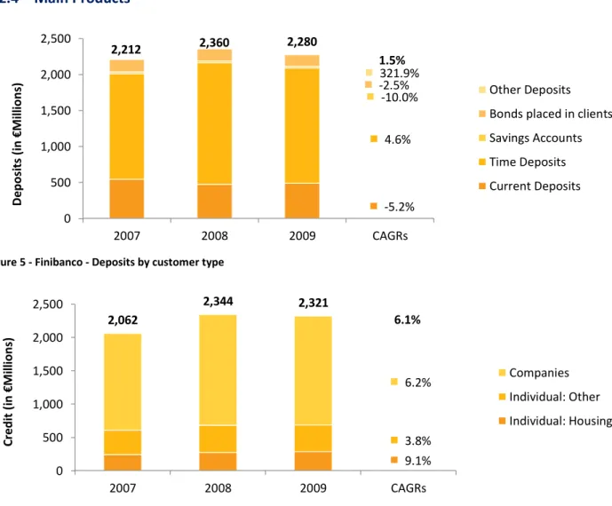
4.1.3 Main Products

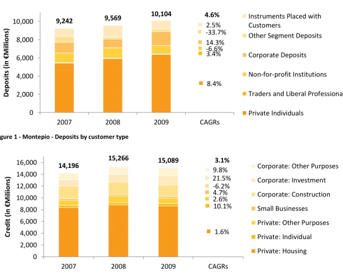
Figure 1 - Montepio - Deposits by customer type

Figure 2 - Montepio - Credit by customer type

As can be seen from the graphs above, Montepio’s major group of clients is private individuals, which accounts for more than 70% of the amount deposited in the three years of the analysis. Also, it is to this group of clients that Montepio lends typically around 66% of the total credit granted.

8.4% 3.4% -6.6% 14.3% -33.7% 2.5% 9,242 9,569 10,104 4.6% 0 2,000 4,000 6,000 8,000 10,000 2007 2008 2009 CAGRs D e p os it s (i n € M ill ion s)

Instruments Placed with Customers

Other Segment Deposits Corporate Deposits Non-for-profit Institutions Traders and Liberal Professionals Private Individuals 1.6% 10.1% 2.6% 4.7% -6.2% 21.5% 9.8% 14,196 15,266 15,089 3.1% 0 2,000 4,000 6,000 8,000 10,000 12,000 14,000 16,000 2007 2008 2009 CAGRs C re d it ( in € M ili ion s)

Corporate: Other Purposes Corporate: Investment Corporate: Construction Small Businesses Private: Other Purposes Private: Individual Private: Housing

(31)

28 The total amount of deposits increased both in 2008 and 2009. However, there was a significant decrease in the amount of corporate deposits in 2008 (17%) that was completely recovered in 2009 and an even greater decrease in the amount of other segments deposits in 2008 (66%) that was followed by a small increase in 2009, which was not enough to recuperate from the loss suffered in 2008.

In terms of the amounts lent to customers, we can observe a different trend. Although the total amount increased in 2008, it decreased slightly in 2009 (1%). This decrease was mostly supported by the decreases in loans to individuals related to housing and other purposes and to corporate clients related to construction.

4.1.4 Cost-to-Income Ratio

Montepio has had a quite stable cost-to-income13 ratio during the period 2007-2009, with values slightly above 60% for the first two years and a value around 55% for the third. This decrease reflects a higher increase in banking revenue (11.7%) than in operating costs (1.1%) and shows an improvement in the operational efficiency of the bank.

In this section, we will discuss the structures of cost and income that yield the ratios mentioned above.

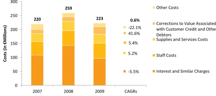
4.1.4.1 Cost Structure

Figure 3 - Montepio - Cost Structure

13_{Here, I use the values obtained in Montepio Annual Reports, which were calculated with the following formula:}

7.5% 44.4% -0.4% -0.7% 872 1,224 1,030 8.7% 0 200 400 600 800 1,000 1,200 2007 2008 2009 CAGRs C os ts (i n € M ill ion s) Other Costs Staff Costs

Corrections to Value Associated with Customer Credit and Other Debtors

(32)

29 As would be expected from a bank, the most relevant costs are related with interest and similar costs, which, in the case of Montepio, account for more than 58% of total costs in any of the three years studied. These costs increased around 15% between 2007 and 2009, having however reached a maximum in 2008. This increase in interest costs is partly justified by a similar in magnitude increase in the total amount of liabilities, maintaining the interest and similar costs/total liabilities ratio fairly constant around 3.3% between the years of 2007 and 2009. However, in 2008, the increase in interest costs was greater than that of total liabilities and this ratio increased to 5%. This, in my view, is a consequence of the financial crisis that intensified with the default of Lehman Brothers in September of 2008 and reflects the greater difficulty in accessing the credit markets for the Portuguese government and banks and the consequent higher yields paid by the issuing institutions.

The second most important source of costs is costs related with impairment, which represent between 8% and 15% of the total costs in these three years. Out of the total impairment costs, more than 75% are loans impairment. It is also important to mention that this kind of impairment doubled between the years of 2007 and 2009, both in absolute and relative terms (in 2007, 1.43% of the total amount of loans was in impairment, whereas in 2009 the impaired loans represented 2.7% of the total amount). Once again, this increase is mostly due to the financial crisis that decreased the power of purchase and shrank the family budget of the Portuguese people.

Another important source of costs is costs with staff. This should also be expected from a firm that provides services, which is the case of banks. These costs decreased slightly between the years of 2007 and 2009, which is probably due to the small decrease in the number of employees, observed in this period14.

Together, these costs account for more than 85% of the total.

14

The number of employees decreased from 2,989 in 2007 to 2,972 in 2008 and increased to 2,986 in 2009. However, one can guess that the new employees hired in 2009 bear smaller costs for Montepio than those who left the bank in 2008.

(33)

30

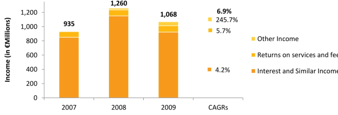
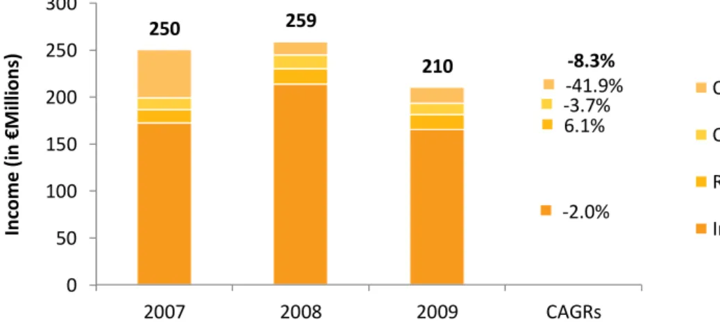
4.1.4.2 Income Structure

Figure 4 - Montepio - Income Structure

Similarly to what was said about the costs with interest and similar expenses, one can also expect from a bank that the main source of income is interest and similar income. One can especially say this about Montepio after running the analysis of amounts in credit and deposits in section 4.1.3, where it was possible to see that Montepio is quite balanced between its lender and borrower sides. Nonetheless, Montepio lends more than it borrows, which, together with the gap between the interest rates applied for each case, allows for a positive net interest income.

Montepio’s income from interest and similar represents more than 85% of the total income for each of the three years and is followed by income from services and fees15 which represent slightly more than 6.5%.

4.1.5 Profits

The profits generated by Montepio witnessed a behavior that would be expected in a crisis scenario: they suffered a big decrease from 2007 to 2008 (almost 45%) and recovered slightly in 2009. However, the value for 2009 is still less than 60% of that for 2007.

4.1.6 Funding

As in any firm, the two main methods of funding of a bank are debt and equity. However, since the business of a bank consists of borrowing at a given interest rate to lend at a higher one and make profits from the

15_{Income from services and fees comprises income from credit fees, means of payment management, insurance and}

cards, among others

4.2% 5.7% 245.7% 935 1,260 1,068 6.9% 0 200 400 600 800 1,000 1,200 2007 2008 2009 CAGRs In co m e ( in € M ill ion s) Other Income

Returns on services and fees Interest and Similar Income

(34)

31 difference, it is typical of a bank to have high levels of debt. Montepio is no exception and shows levels of debt around 95% of the total liabilities and equity.

The main sources of funding are resources from customers and other loans, debt securities issued and deposits from other credit institutions. Together, these types of liabilities account for more than 80% of the total liabilities and for more than 75% of the total liabilities and equity.

It is also relevant to mention the amounts that CEMG borrowed from Central Banks. The evolution of these loans contracted by Montepio clearly reflects the evolution of the liquidity crisis. In 2007, Montepio had no loans from Central Banks; in 2008, this amount was around €850 million with both maturities of up to 3 months and 3 to 6 months; and, in 2009, this amount was of €500 million with maturity of more than 6 months.

About the equity, the only relevant form of equity is share capital, which represents more than 72% of the total equity.

4.1.7 Capital Requirements

Montepio has shown, during the period 2007-2009, a positive trend when it comes to the values of the prudential ratios: the Core Tier 1 Ratio went from 6.4% in 2007 to 9.8% in 2009 and the Solvency Ratio went from 8.89% in 2007 to 13.56% in 2009.

4.1.8 Dividends

The amount of dividends paid by CEMG to AM changed considerably during the period 2007-09, both in absolute terms and in relation to the amount of profit generated in the respective year: the dividends paid were 26, 11 and 20 million euros in 2007-09, which corresponds to dividend payout ratios of 40%, 32% and 54%, respectively. This big variation makes it quite hard to predict both the amount and ratio of dividends paid in the future and justifies why the dividend discount model will not be used in the valuation section.