www.atmos-chem-phys.net/11/7955/2011/ doi:10.5194/acp-11-7955-2011
© Author(s) 2011. CC Attribution 3.0 License.
Chemistry
and Physics
Lake breezes in the southern Great Lakes region and their influence
during BAQS-Met 2007
D. M. L. Sills1, J. R. Brook2, I. Levy2, P. A. Makar2, J. Zhang2, and P. A. Taylor3
1Cloud Physics and Severe Weather Research Section, Environment Canada, Toronto, Ontario, Canada
2Air Quality Research Division, Science and Technology Branch, Environment Canada, Toronto, Ontario, Canada 3Department of Earth and Space Science and Engineering, York University, Toronto, Ontario, Canada
Received: 13 December 2010 – Published in Atmos. Chem. Phys. Discuss.: 1 February 2011 Revised: 22 July 2011 – Accepted: 25 July 2011 – Published: 5 August 2011
Abstract.Meteorological observations from the BAQS-Met field experiment during the summer months of 2007 were in-tegrated and manually analyzed in order to identify and char-acterize lake breezes in the southern Great Lakes region of North America, and assess their potential impact on air qual-ity. Lake breezes occurred frequently, with one or more lake breezes identified on 90 % of study days. They affected all parts of the study region, including southwestern Ontario and nearby portions of southeast Lower Michigan and northern Ohio, with lake-breeze fronts occasionally penetrating from 100 km to over 200 km inland. Occurrence rates and pen-etration distances were found to be higher than previously reported in the literature. This comprehensive depiction of observed lake breezes allows an improved understanding of their influence on the transport, dispersion, and production of pollutants in this region.
The observational analyses were compared with output from subsequent runs of a high-resolution numerical weather prediction model. The model accurately predicted lake breeze occurrence and type in a variety of synoptic wind regimes, but selected cases showed substantial differences in the detailed timing and location of lake-breeze fronts, and with the initiation of deep moist convection. Knowledge of such strengths and weaknesses aids in the interpretation of results from air quality models driven by this meteorological model.
Correspondence to:D. M. L. Sills (david.sills@ec.gc.ca)
1 Introduction and motivation
The Border Air Quality and Meteorology Study (BAQS-Met) was conducted during the summer of 2007 in the southern Great Lakes region of North America to investigate the im-pacts of mesoscale1boundary-layer phenomena, particularly lake breezes, on local air quality and the regional transport of pollutants. A mesoscale monitoring network operated from 1 June to 31 August while a measurement-intensive field cam-paign was carried out from 20 June to 10 July.
The monitoring network comprised existing meteorolog-ical and air chemistry stations plus a number of special surface stations for collecting data with high temporal and spatial resolution. During the intensive observation period (IOP), a variety of additional meteorological and air chem-istry measurements were made by aircraft, via vehicle-based laboratories, and at three “supersites”. The study domain and monitoring network are shown in Fig. 1.
BAQS-Met builds upon previous work in southern On-tario and southeast Michigan related to lake breezes and air quality. Field studies were conducted in 1992–1993 (SON-TOS/SEMOS – Reid et al., 1996; Wolff and Korsog, 1996; Sills, 1998; Hastie et al., 1999), in 1997 (ELBOW 97 – King and Sills, 1998; Sills, 1998), and in 2001 (ELBOW 2001 – Sills et al., 2002). These observational studies fur-thered knowledge of lake breezes and/or air quality problems (particularly with respect to ozone) in the region. However, BAQS-Met was focused on providing a more comprehen-sive understanding through both observations and numerical modelling, and by including the formation and transport of particulate matter such as PM2.5.
1Mesoscale is defined by Fujita (1981) to represent the spatial
Fig. 1.Map showing the BAQS-Met study domain and fixed monitoring network. Light brown lines indicate urban boundaries. The terrain is generally flat to gently rolling and land use is predominantly agricultural with the exception of large urban/industrial areas (e.g. Detroit and Cleveland).
The main questions that this paper attempts to answer are as follows.
1. To what extent do mesoscale meteorological processes such as lake-breeze circulations have the potential to influence air quality in the study region? This is ad-dressed by reviewing the significant impacts that lake breezes are known to have on local and regional air quality, and then demonstrating the degree to which lake breezes influenced the meteorology of the study region during BAQS-Met. Lake breeze characteristics such as occurrence frequency, start/end time intervals, response to various synoptic wind2regimes, and inland penetra-tion distances are examined using an approach that inte-grates complementary observations, providing a highly detailed depiction of lake breeze behaviour in the study region.
2For this study, the 850 hPa wind is used to represent the
large-scale “synoptic” wind and is categorized as follows: light (0.5– 4.9 m s−1), moderate (5.0–9.9 m s−1)and strong (=10.0 m s−1). A synoptic wind less than 0.5 m s−1is considered calm.
2. Does a high-resolution numerical model currently used for air quality research and weather/air quality forecast-ing adequately represent the lake breeze meteorology observed during the study? Here, we assess the abil-ity of a high-resolution numerical weather prediction (NWP) model to generate lake breezes matching obser-vations made during the BAQS-Met IOP. Such a meteo-rological model can be used to drive air chemistry mod-els for air quality research, regulation, and forecasting. However, it must be accurate in order for the transport, dispersion, and production of pollutants to be properly simulated.
Only meteorological processes are examined in this study. However, other studies that investigate air quality and its relation to lake breezes during BAQS-Met (Hayden et al., 2011; Levy et al., 2010; Makar et al., 2010b) are discussed.
case studies (Sect. 5). Results are discussed in Sect. 6 and conclusions are provided in Sect. 7.
2 Background
2.1 Lake-breezes
Lake breezes, like sea breezes, are driven by the difference in pressure between warmer air over land and cooler air over water. Such temperature contrasts are the result of differ-ences in heat flux for land and water surfaces. Lake breezes usually develop a few hours after sunrise and dissipate near sunset, and where present strongly influence the meteorology through the lowest layers of the atmosphere.
Figure 2 shows a cross-section through an idealized lake-breeze circulation in a calm synoptic wind regime. The branches of the circulation include an inflow layer deliver-ing cool marine air, a narrow updraft region at the leaddeliver-ing edge of the inflow layer (called the lake-breeze front), and a descending return flow that generates a subsidence inver-sion. While the inversion suppresses the development of convective clouds above most of the circulation, lift at the lake-breeze front often results in a narrow band of enhanced convective cloud growth (Segal et al., 1997).
The narrow zone of convergence and upward vertical mo-tion at the lake-breeze front can rapidly transport pollutants and help to initiate deep moist convection (DMC), including thunderstorms (especially where lake-breeze fronts merge, intersect or interact with other lift-generating mesoscale fea-tures). The passage of the lake-breeze front is frequently associated with a sharp decrease in temperature, a sharp in-crease in dew point, and a rapid shift to onshore winds. How-ever, the arrival signature in the temperature and dew point data typically becomes more subtle with increasing inland distance due to the rapid modification of the marine air mass over land (Lyons, 1972). This is shown by the growth of the thermal internal boundary layer (TIBL) in Fig. 2.
Physick (1976) found by numerical simulation that, for gulfs and lakes roughly the size of the Great Lakes or smaller, circulations on each shoreline do not occur independently but interact to form a mesoscale high pressure area with associ-ated subsidence over the water. This result has been con-firmed by Estoque (1981) and Comer and McKendry (1993), among others, and probably represents the most significant difference between the dynamics of lake breezes and the dy-namics of sea breezes associated with much larger bodies of water.
When the synoptic wind is light to strong, it deforms the lake-breeze circulation relative to the calm synoptic wind case via two different effects. First, the marine boundary layer and surrounding convective mixed layers are displaced downwind by the synoptic wind, with the displacement in-creasing with the strength of the synoptic wind. Hence, the thermal contrast that causes the lake breeze is also displaced
Fig. 2. Vertical cross-section diagram showing an idealized lake-breeze circulation penetrating inland in a calm synoptic wind regime. Arrows show air motions within and adjacent to the lake-breeze circulation. A thermal internal boundary layer (TIBL) is shown growing in vertical extent with distance inland behind the lake-breeze front (blue dashed line). Magenta lines indicate the lifting condensation level (LCL), green outlines indicate entrain-ment zones, and orange outlines indicate capping inversions. Air motions, various layers, and circulation depth are from Ogawa et al. (1986), Stull (1988), and Lyons (1972), respectively.
downwind (Bechtold et al., 1991). It is worth noting, how-ever, that this displacement affects upwind and downwind shorelines more than shorelines aligned with the synoptic wind, where there may be little relative change in the ther-mal contrast.
Second, the synoptic wind causes the lake-breeze circula-tion to become asymmetrical, with parcel trajectories that are considerably different than those in the calm synoptic wind case (Bechtold et al., 1991; Banta et al., 1993; Atkins and Wakimoto, 1997). Deformation of the lake-breeze circula-tion is discussed in more detail in Sect. 4.3.
Touma, 1981), though more recently Sills (1998) reported penetration distances up to 120 km. Though not explicitly stated, distances approaching 100 km were also suggested in the analyses of lake breezes by Comer and McKendry (1993) and King et al. (2003).
2.2 Impacts on air quality
The exacerbation of air pollution problems in coastal envi-ronments is well known. One of the commonly occurring effects related to the onshore flow of relatively cool marine air is fumigation of pollutants downwind of the shoreline. Effluent from a smokestack at the shoreline blown inland by onshore winds may be confined to a plume in the stably strat-ified marine air. However, as this plume intersects the con-vective mixed layer inland, pollutants can be mixed down to the surface (Lyons and Cole, 1973).
Another commonly occurring effect in coastal areas is plume trapping. Stably stratified marine air moving onshore can have a mean mixing depth that is 10 % of that exist-ing away from the influence of the lake (Lyons and Cole, 1973). Thus, effluent that is emitted into this layer is effec-tively trapped and high concentrations of pollutants can sub-sequently reach the surface and persist. In addition, under such conditions high concentrations of precursors and sec-ondary pollutants can be sustained for longer times and over larger transport distances. This can influence chemical re-actions and result in the formation of a greater quantity of ozone, for example.
Fumigation and plume trapping often occur in association with lake breezes. However, lake breezes introduce their own unique problems. The first is the ability of lake-breeze cir-culations to transport pollutants in three dimensions. For ex-ample, pollutants emitted into the inflow layer travel inland, are lofted in the frontal region, and then disperse into the flow aloft. A fraction of these pollutants may enter the in-flow layer again, and can follow a helical trajectory along the shoreline (Lyons and Olsson, 1973; Lyons and Cole, 1976; Lyons et al., 1995; Harris and Kotamarthi, 2005). This will be discussed in more detail in Sect. 4.3.
Another effect on air pollution often occurring with lake breezes involves the increased production of ground-level ozone or “photochemical smog”. The ingredients for delete-rious ground-level ozone concentrations include an abundant supply of volatile organic compounds (VOCs) and oxides of nitrogen (NOx), strong insolation, relatively high air temper-atures, light wind speeds, and limited mixing depths (Lyons and Cole, 1976). Three of these ingredients – strong insola-tion, relatively high temperatures over land, and light winds – are also conditions associated with the development of vig-orous lake breezes. When a lake breeze does develop, cloud-less skies, enhanced insolation, and limited mixing depths are common over the lake and at inland locations behind the lake-breeze front (see Fig. 2) and can result in increased ozone production there given the availability of precursors.
This ozone can then be advected inland by the lake breeze, as has been shown by Hastie et al. (1999).
Though a strong relationship between sea/lake breezes and photochemical smog has been demonstrated by Gusten et al. (1988), among others, there are also situations when the sea/lake breeze delivers relativelycleanair to a region expe-riencing photochemical pollution (e.g. Hayden et al., 2011; Levy et al., 2010).
3 Data and methodology
3.1 Observational data
A number of observational data sets were utilized for this study, including surface weather station data, GOES-8 vis-ible channel satellite imagery, and weather radar imagery. There were a total of 54 surface weather stations operating in the BAQS-Met study region during the June to August pe-riod. Thirty-eight of those were existing stations operated by various agencies such as Environment Canada, the US Na-tional Weather Service, and the Ontario Ministry of the En-vironment, and these provided data hourly. The remaining 16 surface stations were installed for BAQS-Met, including 12 from Environment Canada (with a buoy in each of Lake Erie and Lake St. Clair) and four from York University (see Fig. 1). Averaged data from these stations were provided at 1 min intervals.
The bulk of these stations made measurements at World Meteorological Organization standard heights of 10 m for wind and 1.5 m for temperature and dew point. Pressure, solar radiation, and precipitation were also measured at a number of sites. Data from these fixed surface stations were supplemented by mobile observations over land and ship ob-servations over the lakes when available.
All available GOES-8 visible and infrared channel satel-lite images were collected, mainly at 15 min intervals. Lake surface temperature data based on infrared measurements from the NOAA POES polar-orbiting satellite were ob-tained from the Great Lakes Environmental Research Lab-oratory (GLERL) Great Lakes Surface Environmental Anal-ysis (GLSEA) dataset (Schwab et al., 1992).
Finally, to determine synoptic wind regime characteristics during the study period, the 850 hPa wind at 20:00 local time (LT, equivalent here to 20:00 EDT and 00:00 UTC) from the closest rawinsonde station (DTX) northwest of Detroit, Michigan, was used (see Fig. 1 for location). In cases where the 850 hPa wind was not available at 20:00 LT, or precipita-tion was falling at DTX in the hour preceding 20:00 LT, the 08:00 LT (12:00 UTC) sounding was used. In addition, DTX data were not available for the last three days of the study, so 20:00 LT data from the BUF rawinsonde near Buffalo, New York, to the east of the study region were used instead.
3.2 High-resolution numerical model
The Global Environmental Multiscale (GEM) model, de-scribed by Cˆot´e et al. (1998), is an NWP model used for oper-ational forecasting by Environment Canada. A limited-area version of this model (GEM-LAM) having approx. 2.5 km horizontal grid spacing and 58 hybrid-coordinate levels in-creasing monotonically with height from the Earth’s surface to 10 hPa was used to simulate the meteorological condi-tions observed during the BAQS-Met IOP. These meteoro-logical fields were also used to drive a regional air pollution modeling system known as AURAMS (A Unified Regional Air-quality Modeling System, see Makar et al., 2010a, b). Most of the initial and boundary conditions for these high-resolution runs were provided by a global variable-high-resolution version of the GEM model using approx. 15 km horizontal grid spacing in the core region and the same vertical coordi-nates as the high-resolution simulation. High-resolution geo-physical fields, and high-resolution lake surface temperatures based on climatological values, were exceptions. Initial and boundary conditions for the coarse grid model runs were pro-vided by operational data-assimilated analyses. See Makar et al. (2010a) for more details.
3.3 Identification of lake breezes in observational data
One of the defining features of a sea-breeze circulation is the formation of a sea-breeze front (Physick, 1976) though, as discussed earlier, it is recognized that a front may not de-velop under strong synoptic wind regimes. Accordingly, nu-merous studies have used the detection of the front as a pri-mary criterion when identifying sea- or lake- breeze circu-lations (e.g. Lyons, 1972; Ryznar and Touma, 1981; Atkins and Wakimoto, 1997; Sills, 1998; Laird et al., 2001; Zumpfe and Horel, 2007). Improvements in the resolution and tem-poral frequency of data from radar, satellite and surface ob-servation networks have made detection of such fronts less difficult, so efforts have become increasingly focused there.
Hence, for this study, we have used a methodology that relies primarily on lake-breeze front identification to gener-ate analyses and statistics describing lake breeze behaviour during the study period. Mesoscale meteorological analy-ses were generated for each day of the study using the
Au-rora workstation (Greaves et al., 2001). Surface weather sta-tion data, GOES-8 satellite visible channel imagery, and low-level radar reflectivity/radial velocity data were displayed si-multaneously and visually inspected, both at hourly inter-vals and via animations. For days during the IOP, the es-timated positions of identified lake-breeze fronts were in-corporated into the hourly analyses, as were synoptic-scale front positions obtained from operational weather analy-ses. Animations of hourly mesoscale analyses for each day of the IOP are available on the web at http://tinyurl.com/ SillsBAQS-MetAnimations.
Table 1 lists the criteria used to identify lake breezes. Pos-itive factors were those that gave evidence of a lake-breeze front, such as a line of cumulus clouds and/or radar fine line quasi-parallel to the shore3moving gradually inland (but not associated with a DMC gust front or synoptic-scale front). Negative factors, such as the absence of onshore flow evi-dent in the surface data, were used to reject the case for a lake breeze. In addition, evidence for a lake breeze from a single observation platform could sometimes be ambiguous, such as there being no cloud present on visible satellite im-agery. In such cases, more weight was placed on evidence from the other observational platforms.
In situations where the passage of a lake-breeze front could not be confirmed via the mesoscale analysis, time se-ries of 1 min data from individual surface stations were ex-amined for rapid changes in wind, temperature and/or dew point not associated with DMC gust fronts or synoptic-scale fronts. A similar factor-based methodology was used to iden-tify other mesoscale boundaries such as land-breeze fronts and DMC gust fronts. These were added to hourly mesoscale analyses when present during the IOP.
Figure 3 is a mesoscale analysis valid at 15:00 LT on 6 July 2007 that includes the estimated positions of lake-breeze fronts. In parts of the study region at this time, such as in the vicinity of Lake St. Clair, the locations of lake-breeze fronts are clear. There are sharp wind shift lines, cumulus cloud lines and edges, and radar fine lines (these are some-what obscured by the front symbols). There are other areas where locating the lake-breeze front was not as straightfor-ward. Southwest of Lake Huron and west of Lake Erie, there are surface observations on only one side of the lake-breeze front, so a wind shift line is not observed. However, in both cases, enhanced growth at the edge of the cumulus cloud field is apparent. These cloud lines/edges are even more ev-ident when the plots are animated. Lastly, there are areas where the evidence points to there being no lake-breeze front present. Southeast of Lakes Huron and Erie, winds are on-shore but cumulus clouds appear to gradually deepen with inland distance, indicating a growing convective mixed layer rather than a cloud edge associated with a lake-breeze front. In these areas, the lake breeze has no distinct leading edge.
3Note that “shore” as defined for this study consists only of the
Table 1. Lake breeze identification criteria based on three different observation platforms, including positive, negative, and ambiguous factors.
Platform Positive Factors Negative Factors Ambiguous Satellite
(visible channel)
– line of cumulus clouds or sharp gradient in cumulus cloudiness quasi-parallel to shore
– gradual inland penetration of above, or quasi-stationary
– persistent thick cloudiness over most or all of lake area – gradual change in the depth of cumulus clouds inland from lake (gradually deepening con-vective mixed layer)
– no cloud visible
– thin cirrostratus or broken mid-level clouds prevents seeing cumulus clouds
Radar (reflectivity, radial velocity)
– fine line or sharp gradient in clear-air echoes quasi-parallel to shore
– shift in radial velocity along fine line – gradual inland penetration of above, or quasi-stationary
– large area of persistent precipitation over region
– no clear air echoes – fine line or gradient in clear-air echoes not well defined
Surface (station plots, time series)
– rapid shift in wind direction to onshore wind (may be accompanied by rapid change in wind speed, sharp decrease in temperature and dew point within 20 km of shore)
– gradual inland penetration of onshore winds
– elongated area of convergence quasi-parallel to shore
– gradual inland penetration of above, or quasi-stationary
– no onshore winds – often very subtle surface gradients at boundaries in moderate/strong synoptic wind regimes
– an area of broad
divergence over the lake and the adjacent shore often indicates that a lake-breeze circulation is present and may be used to sup-port the presence of a
lake-breeze front
The chosen study domain makes it very difficult for a lake breeze to occur on one of the lakes without an associ-ated lake-breeze front somewhere in the domain. For exam-ple, a Lake Erie lake breeze in a moderate southerly syn-optic flow does not typically result in a lake-breeze front on the north shore, but a lake-breeze front does develop on the south shore. Even in a northerly synoptic flow, with no northern Lake Huron shoreline present in the study domain, lake-breeze fronts typically form along either the eastern or western shore of the southern part of Lake Huron. In ad-dition, through the study period, there were no days when lake breezes were prevented from developing due to a strong synoptic wind. Therefore, given the above, we believe that all lake-breeze circulations occurring during the study period could be identified via detection of a lake-breeze front.
Errors in the analyzed positions of lake-breeze fronts de-pended on data type and density. In periods/regions with only low-density surface data available for identification, the error might be as large as±10 km. When visible satellite imagery was used for identification, factors such as cloud line dis-placement relative to the front and parallax due to the 45◦ satellite viewing angle resulted in errors estimated to be as large as±5 km. Radar fine lines resulted in the most accurate analyzed lake-breeze front positions, estimated to be within ±1 km. However, fine lines were not visible on all days, and when present were usually apparent only within 100 km of a
radar. The ability to integrate data from each of these plat-forms in space and time using the Aurora workstation often helped to reduce overall positional error considerably.
The manual lake breeze identification process described above is labour intensive and relies on pattern recognition skills. However, there are numerous examples of this type of mesoscale boundary analysis undertaken in both in a re-search setting (Purdom, 1976; Ryznar and Touma, 1981; Wilson and Schreiber, 1986; Hastie et al., 1999; Roebber and Gehring, 2000; Laird et al., 2001; King et al., 2003; Sills et al., 2004; Wilson and Roberts, 2006) and a real-time set-ting (Wilson et al., 2004, 2010; Sills and Taylor, 2008). The results should be replicable given substantial knowledge of and experience with meteorological data analysis.
Fig. 3.Mesoscale analysis showing low-level radar echoes (mainly green), visible satellite imagery, surface observations, and the positions of lake-breeze fronts (broken magenta lines) for 15:00 LT on 6 July 2007. Long wind barbs are 5 m s−1, short barbs are 2.5 m s−1.
3.4 Identification of lake breezes in GEM-LAM output
GEM-LAM output was examined using the Unidata Inte-grated Data Viewer (IDV) (Murray et al., 2003). As with the observational data, identification of a lake breeze pri-marily involved locating a lake-breeze front. Lake-breeze fronts were identified by superimposing vertical velocity on the surface wind field. Elongated regions quasi-parallel to shore having upward vertical velocity greater than 0.1 m s−1 at 390 m a.g.l. and surface wind convergence (not related to convective downdrafts and synoptic-scale fronts) were deter-mined to be lake-breeze fronts if surface winds behind the front were onshore. Vertical velocity at the 390 m model level was used because it was found to best represent the maximum updraft at the lake-breeze front, and the 0.1 m s−1 threshold was employed to filter out numerous regions of weak lift. Animations of the surface wind and vertical ve-locity fields in IDV often made identification of lake breezes straightforward.
Figure 4 shows an example plot used for lake breeze iden-tification valid at 15:00 LT on 6 July 2007. It includes the estimated positions of lake-breeze fronts derived from the model data. Errors in the analysis of simulated lake-breeze front positions at the surface were overall less than that for observed lake-breeze fronts and depended mainly on the pos-sible displacement between the surface convergence and the
1
Fig. 4.GEM-LAM surface winds (long barb=5 m s−1, short barb
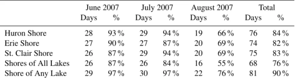
Table 2.The number and percentage of days per month with observed lake breezes, plus the total number and percentage for all study days. Values are grouped by shore categories.
June 2007 July 2007 August 2007 Total Days % Days % Days % Days % Huron Shore 28 93 % 29 94 % 19 66 % 76 84 % Erie Shore 27 90 % 27 87 % 20 69 % 74 82 % St. Clair Shore 26 87 % 29 94 % 20 69 % 75 83 % Shores of All Lakes 26 87 % 26 84 % 16 55 % 68 76 % Shore of Any Lake 29 97 % 30 97 % 22 76 % 81 90 %
lift at 390 m, resulting in an estimated error up to ±2 km. Note that this representsanalysiserror and does not account formodelerror, which can be much larger (as discussed in Sect. 6).
The model daily penetration distance for each lake was calculated for the hour showing the maximum inland pene-tration of the lake-breeze front. The distance selected was the furthest extent of the front from the lake, measured to the closest point along the shoreline. Note that the distance to the lake-breeze front was calculated even if the front had moved outside of the study region. Values rounded to the nearest 5 km are reported.
4 Results from the June–August period
A number of observed lake breeze characteristics are derived and compared in this section, covering the months of June through August, 2007. They include lake breeze occurrence frequency, start/end time intervals, and the influence of the synoptic wind. Each of these is important for gaining a better understanding of the behaviour of summer lake breezes in the study region and determining their influence on air quality, as discussed in the Sect. 2. Derived data for each day are provided in the Supplement, Table S1.
4.1 Observed occurrence frequency
Table 2 shows lake breeze occurrence frequencies grouped by shore category for 90 of 92 days (data were not properly archived for two days – 18–19 August). Lake breezes were identified on at least one shore on 90 % of study days. Each of the individual lakes generated a lake breeze in the study region on between 82 % and 84 % of days. On 76 % of days, lake breezes occurred simultaneously on all shores. Between 4 June and 4 August, inclusive, there was only one day with-out a lake breeze somewhere in the study region. In addition, there were three periods with lake breezes on all shores oc-curring over 11 consecutive days or more (8 June–18 June, 20 June–10 July, 21 July–4 August) with the longest being 21 days (fortuitously, the BAQS-Met IOP was during this pe-riod). The Lake Huron shore had 24 consecutive lake breeze
days between 20 June and 13 July. This is twice the highest number of consecutive lake breeze days previously reported (12 days for Lake Michigan; Eichenlaub, 1979).
The lake breeze frequencies found here are higher than those reported by other researchers in the Great Lakes region. Comer and McKendry (1993) estimated a 30 % lake breeze frequency for Lake Ontario, but over a period from April to September, inclusive. Lyons (1972) and Laird et al. (2001) examined lake breeze occurrences on the east and west sides of Lake Michigan and found combined frequency values dur-ing the summer months of 46 % and 62 %, respectively.
A check was performed to see if this difference in observed lake breeze frequency could be explained by weather con-ditions during the summer of 2007. During this study, the greatest limiting factor for lake breeze occurrence was the presence of thick clouds and precipitation, typically associ-ated with a passing low-pressure system. Therefore, a clima-tological comparison was used to indicate how often the area was affected by weather conditions resulting in precipitation and related reduced temperatures.
Precipitation and temperature records were examined for the June through August period at the Windsor Airport cli-mate station (monthly cloud cover values were not available). It was found that the average mean and maximum tempera-tures for the period were both 1.2◦C higher than the 1971–
2000 climate normals, while the number of days with rainfall was 30.0 compared to the normal of 31.2 (see Table 3). Dur-ing July, the month with the greatest overall lake breeze oc-currence during BAQS-Met, temperatures were exactly nor-mal and the number of days with rain was only about 10 % below normal. This appears to show that larger-scale condi-tions during summer 2007 were not responsible for the differ-ence between the lake breeze occurrdiffer-ence during the summer months of 2007 and that found in previous studies.
Table 3.Climatological averages for June, Jul and August 2007 compared to climatological normals. Data are from Environment Canada’s historical weather web portal found at http://www.climate.weatheroffice.gc.ca.
June July August June–August 2007 Normal 2007 Normal 2007 Normal BAQS-Met Normal Max Temp (◦C) 27.7 25.4 27.9 27.9 27.7 26.6 27.8 26.6 Mean Temp (◦C) 22.1 20.1 22.7 22.7 23.3 21.6 22.7 21.5 Days with Rainfall 9.0 11.0 9.0 10.2 12.0 10.0 30.0 31.2
can be explained by the lake breeze identification criteria used for past studies. Both Comer and McKendry (1993) and Laird et al. (2001) required no synoptic-scale frontal pas-sages in the region of interest. Comer and McKendry (1993) required that the sky be clear or partly cloudy during daylight hours. Lyons (1972) required the presence of a return flow above the inflow layer.
Applying these criteria to the BAQS-Met data would elim-inate a large number of lake breeze occurrences. Lake breezes were observed to occur in the presence of a synoptic-scale front in the domain on 18 days (there were 24 days with at least one front in the study domain during daytime hours, 18 with lake breezes). On 42 days, lake breezes were experi-enced in areas with more than three hours of mostly cloudy or overcast conditions (as revealed by visible satellite imagery). This cloud was often associated with arriving or departing precipitation, or a thin or broken deck of mid- or upper-level cloud. Occasionally the cloudy conditions were produced by DMC initiated at the lake-breeze fronts themselves. Finally, during intensive observations when air above the lake breeze inflow layer could be sampled by aircraft, it was found that a return flow was often difficult to discern (see Hayden et al., 2011). This is likely true in most cases with a moderate to strong synoptic wind (Moroz, 1967; Banta, 1993).
4.2 Start and end time intervals
The first and last hours on which lake-breeze fronts were de-tected each day are included in the Supplement, Table S1. From these, observed lake breeze start and end time inter-vals are determined. One-hour interinter-vals were used since the mesoscale analyses were only available every hour. The start time interval is the first hour interval over which a lake-breeze front could first be observed on any shore (e.g. the interval 09:00–10:00 LT indicates a lake-breeze front first identified at 10:00 LT). The end time interval is the last hour interval over which lake-breeze fronts could be observed on any shore (e.g. the interval 20:00–21:00 LT indicates a lake-breeze front last identified at 20:00 LT). The lake lake-breeze du-ration using the examples above would be 11 h.
In addition, a number of studies have found that sea-breeze fronts moving inland after sunset often do so in the form of a detached vortex no longer connected to an active sea-breeze
circulation (e.g. Simpson et al., 1977; Sha et al., 1993). This was found to be the case for six days during the study period (marked in the Supplement, Table S1). On these days, one or more detached lake-breeze fronts were detected after sunset when lake-breeze circulations had dissipated. This mainly involved the Lake Huron lake-breeze front penetrating south and west of Lake St. Clair. Therefore, for this analysis, the hour that the lake-breeze front was last identified on these days was replaced by the hour over which sunset occurred.
Using the above methodology, the median lake breeze start time interval for the period June to August 2007 was 10:00–11:00 LT, with a range from 08:00–09:00 LT to 18:00-19:00 LT. The median start time interval of 10:00–11:00 LT is the same as the most frequent interval found by Lyons (1972) on the western Lake Michigan shoreline. The medianendtime interval during this period was 20:00–21:00 LT, with a range from 15:00–16:00 LT to 21:00–22:00 LT. The median lake breeze duration was calculated to be 9 h, with a range from 2 h to 13 h.
Lake breeze start and end times can vary widely depending on weather conditions. For example, lake breezes may begin late as cloud associated with a low-pressure system moves out, or may end early if cloud and downdrafts associated with DMC begin to dominate. In addition, there are often small differences in start and end times for each lake but an analysis of this type was not undertaken.
4.3 The synoptic wind and its influence
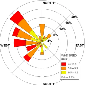
The frequencies of synoptic wind directions and speeds dur-ing the study period are shown in Fig. 5. Synoptic winds from the western quadrant (southwest to northwest) were by far the most frequent. Northwest synoptic winds occurred on 19 % of study days. In contrast, there were no cases with a synoptic wind from the east-northeast, east, or south-southeast. As shown in Fig. 5, light to moderate synoptic winds were observed from most directions, but strong syn-optic winds occurred only from the south-southwest through northwest. Lake breezes occurred in synoptic winds from each observed direction, and with synoptic wind speeds up to 23 m s−1.
1
Fig. 5. Wind rose diagram showing the percent frequency of rawinsonde-derived 850 hPa wind directions (16 bins) and wind speeds (light=yellow, moderate=orange, and strong=red) for 90 days during BAQS-Met. Note that on one day the synoptic wind was calm and that there were no occurrences from the east-northeast, east, or south-southeast.
of deformation related to the synoptic wind speed. Three types of circulation deformation were identified during the BAQS-Met study period: low deformation (LD), moderate deformation (MD), and high deformation (HD). These lake-breeze circulation types are illustrated in Fig. 6.
LD lake-breeze circulations are most similar to the clas-sic “textbook” description of the lake or sea breeze, with lake-breeze fronts observed around the entire perimeter of the lake. The synoptic wind must be weak for this to oc-cur (Lyons, 1972). The front on the upwind shore may be intensified due to an opposing synoptic wind increasing the convergence and the frontal gradient. The front on the down-wind shore may be weakened due to an onshore synoptic wind reducing the frontal gradient, making it more difficult to detect in the observational network. For this study, if a lake-breeze front was positively identified on at least one of the downwind shores of the lakes in the study area, then the lake-breeze circulations on that day were considered LD.
With MD lake-breeze circulations, fronts are observed around the perimeter of the lake except on the downwind shore. There, the onshore synoptic wind prevents even a weak front from forming. The front on the upwind shore reaches a maximum intensity if the inland penetration of the lake-breeze front is offset by the synoptic wind, resulting in a front that is quasi-stationary with respect to the shore. How-ever, if the synoptic wind increases further then the strength
Fig. 6. Diagrams showing low-, moderate-, and high-deformation lake-breeze circulations in plan view. Black arrows are streamlines. Broken magenta lines are lake-breeze fronts. Large arrows at left represent the synoptic wind increasing from top to bottom. The synoptic wind results in a stronger front in magenta-shaded areas, and a weaker front in green-shaded areas.
of the front on the upwind shore decreases (Bechtold et al., 1991). If a lake-breeze front was detected on at least one of the upwind shores of the lakes in the study area, but not on any downwind shores, then the lake-breeze circulations on that day were considered MD.
For HD lake-breeze circulations, the synoptic wind pre-vents the development of fronts on both the upwind and downwind shores, but fronts are still observed along shores parallel to the synoptic wind since thermal contrast is mostly preserved there.
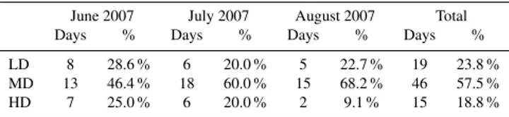
Table 4 shows the occurrence rate for each lake-breeze circulation type, with MD lake-breeze circulations having occurred the majority of the time during the study period (57.5 %), and LD and HD circulations having occurred on 23.8 % and 18.8 % of study days, respectively. To further il-lustrate the differences between these circulation types, one case of each type will be discussed in detail later in Sect. 5.3 (Selected Cases).
Deformation of the lake-breeze circulation significantly changes air parcel trajectories relative to the calm synoptic wind case. For example, along shorelines aligned with the synoptic wind, both the inflow and return flow take on an along-shore component in addition to their cross-shore com-ponent, resulting in a helical flow about the shoreline (Lyons and Olsson, 1973; Lyons et al., 1995). Such trajectories are discussed in Hayden et al. (2011) related to an LD lake-breeze circulation during the BAQS-Met IOP. This helical structure is stretched downwind as the synoptic wind and the along-shore component increase. The potential for recircula-tion of pollutants with MD and HD lake-breeze circularecircula-tions is thus reduced since the time required for a parcel to move onshore to the lake-breeze front then back offshore is also increased.
Additionally, with MD lake-breeze circulations, recircula-tion cannot occur on the downwind shore. Similarly, with HD circulations, no recirculation is possible on both the up-wind and downup-wind shores. Since MD and HD circulations occurred on more than three quarters of days during BAQS-Met study period, the implication is that recirculation of pol-lutants is possible only on a limited number of summer days in the study region, and then is most likely to occur where the shoreline is approximately aligned with the prevailing synop-tic wind.
5 Results from the intensive period
The BAQS-Met IOP ran from 20 June to 10 July 2007. As mentioned earlier, this period was remarkable due to lake breezes being observed simultaneously on all shores each day (see Supplement, Table S1). In this section, observed and GEM-LAM-simulated lake breeze characteristics are de-rived and compared for the IOP, and for three selected cases. The goal is to assess GEM-LAM’s ability to simulate the lake-breeze circulations observed, and assess the accuracy of the meteorological fields that have been used to drive the AURAMS air quality modeling system. Daily details of the lake breezes generated by the GEM-LAM are provided in the Supplement, Table S2.
5.1 General comparisons
GEM-LAM successfully simulated the development of lake breezes on each shore for each of the IOP days. In addition, GEM-LAM accurately captured the lake-breeze circulation
Table 4. Number of days and occurrence frequency for each lake-breeze circulation deformation type over the entire BAQS-Met study period. LD, MD and HD are low deformation, moderate de-formation, and high dede-formation, respectively.
June 2007 July 2007 August 2007 Total
Days % Days % Days % Days %
LD 8 28.6 % 6 20.0 % 5 22.7 % 19 23.8 %
MD 13 46.4 % 18 60.0 % 15 68.2 % 46 57.5 %
HD 7 25.0 % 6 20.0 % 2 9.1 % 15 18.8 %
type for all days except 4 July, when a higher model synop-tic wind resulted in HD circulations rather than the observed MD circulations.
On most IOP days, lake-breeze fronts were identified in the GEM-LAM output at times well after sunset. Similar to the observed lake-breeze fronts discussed in Sect. 4.2, these simulated lake-breeze fronts were likely disconnected from an active lake-breeze circulation, propagating inland as a de-tached vortex. Therefore, as was done for the analysis in Sect. 4.2, on IOP days where the observed and simulated lake-breeze fronts were detected after the time of sunset, the hour that the lake-breeze front was last identified was re-placed by the hour over which sunset occurred.
Using this methodology for IOP days, theobserved me-dian lake breeze start time interval was 10:00–11:00 LT and the median end time interval was 20:00–21:00 LT, with a me-dian duration of 10 h. For theGEM-LAM simulationsover the IOP, the median start time interval was 09:00–10:00 LT, the median end time interval was 21:00–22:00 LT, and the median duration was 12 h.
Part of the reason for the earlier median start time inter-val and later median end time interinter-val from the model is that, with high spatial/temporal resolution and data at all locations, lake-breeze fronts are less difficult to detect than with observational platforms that have spatial/temporal lim-itations (e.g. visible satellite imagery only available during daylight hours).
5.2 Inland penetration of lake-breeze fronts
5.2.1 Observations
lake breeze impacts on air quality in the Great Lakes region extends much further inland than previously thought.
Each of the penetration distance maxima above were recorded when a component of the synoptic wind was on-shore. In general, lake-breeze fronts tended to penetrate further inland in these regimes. Note that, as discussed in Sect. 4.2, lake-breeze fronts propagated inland after sunset as detached vortices on six days during the IOP, and the maxima for the Lake Huron lake-breeze front was observed during one of these days (21 June).
5.2.2 GEM-LAM output
For days during the IOP, the GEM-LAM simulated me-dian inland penetration distances for Lakes Huron, Erie and St. Clair were 120 km, 65 km and 75 km, respectively, while maxima were 245 km, 160 km and 125 km, respectively. The penetration distances from the model are generally greater than those observed during the IOP for reasons discussed in Sect. 5.1. Note that each of the maxima above were recorded for days during the IOP when it is likely that the simulated lake-breeze fronts propagated inland in the evening as de-tached vortices.
5.2.3 17:00 LT penetration distance comparison
To provide a better comparison between the observed and modelled lake-breeze penetration distances that removes any influences related to limited visible satellite imagery and de-tached vortices, maximum inland penetration distances at or before 17:00 LT were obtained for both observed and simu-lated lake breezes (Supplement, Table S3). The penetration distance statistics are compared using a box-and-whiskers format in Fig. 7. The graph shows that simulated Lake Huron lake breezes, like their observed counterparts, penetrated fur-ther inland on average than Lakes Erie and St. Clair lake breezes.
Median distances between 30 km and 50 km are shown for both observed and simulated lake breezes for Lakes Erie and St. Clair. For Lake Huron, however, there is a more clear dif-ference between observed and simulated lake breeze penetra-tion distances, with the median distance for GEM-LAM lake-breeze fronts being 20 km further inland than observed. In fact, the observed median is below the 25th percentile value for the simulated distances.
5.3 Selected cases
In this section, three cases from the IOP will be examined in greater detail. The cases were chosen to represent LD, MD, and HD lake-breeze circulation types, as well as a vari-ety of air quality conditions and levels of convective activity. In each case, the observed evolution of the lake breeze, and in particular the movement of lake-breeze fronts, is qualita-tively compared to the evolution from the GEM-LAM model
0 25 50 75 100 125 150
Huron-Obs Huron-GEM Erie-Obs Erie-GEM St. Clair-Obs St. Clair-GEM
P
en
et
rat
ion D
is
tanc
e (
k
m
)
Penetration Distance Comparison - Observations vs GEM-LAM output
Fig. 7.Box and whiskers diagram comparing observed and GEM-LAM maximum penetration distances at or before 17:00 LT. On each box, the red central mark is the median, the top and bottom of the box are the upper and lower quartiles, respectively, and the whiskers extend to the most extreme data points.
output at three-hour intervals, beginning at 11:00 LT and end-ing at 20:00 LT. Observed and modeled lake breeze interac-tions are also be noted.
5.3.1 23 June 2007 LD lake breezes
The centre of a high-pressure system was located over south-western Ontario in the morning and drifted southeast through the day. While little in the way of low-level cumulus cloud developed over the study region (even along lake-breeze fronts), there was a persistent deck of broken upper-level cir-roform clouds, especially over the southwestern half. The synoptic wind was light, with the 850 hPa wind from the DTX 23 June, 20:00 LT rawinsonde being 180◦ at only
3.6 m s−1. Inland maximum temperatures ranged between
24◦C and 25◦C, while lake surface temperatures ranged
from 13◦C in parts of southern Lake Huron to 24◦C in parts
of western Lake Erie. BAQS-Met measurements on this day indicated good to moderate air quality across southwestern Ontario (daytime maximum ozone in the 30–60 ppbv range). The observed and modeled evolutions of lake breezes on this day are shown in Fig. 8. For both observations and GEM-LAM output, lake breezes developed on all lakes and lake-breeze fronts moved inland from all shores, indicating that LD lake-breeze circulations were present. No DMC was ob-served, or simulated in the model.
Fig. 8.Observed (magenta) and GEM-LAM modeled (blue) features at four different times on 23 June 2007. Solid lines mark Lake St. Clair lake-breeze fronts, dotted lines Lake Erie lake-breeze fronts, and dashed lines Lake Huron lake-breeze fronts. Arrows on panel d show synoptic wind directions and relative synoptic winds speeds for the day. Locations A–C are discussed in the text.
The GEM-LAM 850 hPa wind at 20:00 LT on 23 June was 149◦at 1.9 m s−1, so 31◦further east and 1.7 m s−1less than the observed wind. The GEM-LAM was more aggressive with the inland penetration of the Lake Erie lake breeze early in the simulation. It was also much more aggressive with the inland penetration of the Lake Huron lake breeze toward the southeast, penetrating almost 50 km further inland than ob-served by 17:00 LT. The lower speed of the opposing synop-tic wind in the model likely allowed the increased penetration of the Lake Huron lake breeze.
Both observations and model output indicate that Lakes Erie and St. Clair lake-breeze fronts merged south of Lake St. Clair (marked by “A” in Fig. 8b), and that Lakes Huron and St. Clair lake-breeze fronts merged north of Lake St. Clair (marked by “B” in Fig. 8c). However, only the model output indicated the merger of the Lakes Huron and Erie lake-breeze fronts late in the day (marked by “C” in Fig. 8d).
5.3.2 26 June 2007 MD lake breezes
On this day, the study region was under the influence of a large “Bermuda High” pressure system with an approaching low-pressure system located over southern Manitoba. Clear skies in the morning gave way to shallow low-level cumulus clouds at inland locations, deepening cumulus clouds along lake-breeze fronts, and isolated DMC late in the afternoon mainly south and west of Lake Erie. The 850 hPa wind
from the DTX 26 June, 20:00 LT rawinsonde was 235◦ at
6.7 m s−1. Inland maximum temperatures ranged between 29◦C and 35◦C, while lake surface temperatures ranged from 15◦C in parts of southern Lake Huron to 24◦C in parts of western Lake Erie. BAQS-Met air chemistry measure-ments on this day indicated poor air quality across southwest-ern Ontario (daytime maximum ozone in the 70–100 ppbv range) – the second day in a row with such conditions.
The observed and modeled evolutions of lake breezes on this day are shown in Fig. 9. The observed lake-breeze fronts from Lake Erie and Lake St. Clair penetrated inland approx. 80 km and 70 km, respectively, toward the northeast by 17:00 LT. They moved even further inland by 19:00 LT (not shown) but became undetectable by 20:00 LT. By that time, however, lake-breeze circulations had affected the boundary layer over the entire study region.
Fig. 9. Same as in Fig. 8 but for 26 June 2007. Dotted lines mark surface gust fronts due to deep moist convection (light magenta for observations and light blue for modeled). Locations A–D are discussed in the text.
The development of DMC was both observed and simu-lated by the model south and west of Lake Erie (though the model generated DMC several hours earlier than observed). However, in other areas, the model generated much more DMC than was observed, with DMC downdrafts dominat-ing much of the western half of the study area by 17:00 LT. The locations of DMC gust fronts are included in Fig. 9.
Both observations and model output show that the Lake St. Clair and Lake Huron lake-breeze fronts intersected northwest of Sarnia by 14:00 LT (marked by “A” and “B” in Fig. 9b). However, only the observations indicated the in-tersection of Lakes Erie and St. Clair lake-breeze fronts by 17:00 LT (at two points marked by “C” and “D” in Fig. 9c).
5.3.3 8 July 2007 HD lake breezes
In this case, the study region was located in the warm sector of a low-pressure system whose centre was moving across the northern Great Lakes. A warm front and a cold front were positioned to the northeast and northwest of the study region, respectively. Shallow low-level cumulus clouds developed over northern Ohio and southeast Michigan but not over or downwind from Lakes Erie and St. Clair. Over the northeast part of the study region, there was a persistent area of broken mid- to high-level clouds associated with warm frontal DMC further northeast. This cloud prevented a Lake Huron lake breeze from being detected until late afternoon. However, lake breezes were eventually detected on all shores.
Inland maximum temperatures ranged between 33◦C and
36◦C, while lake surface temperatures ranged from 16◦C in
parts of southeastern Lake Huron to 26◦C in parts of south-western Lake Erie. BAQS-Met measurements on this day indicated poor air quality across southwestern Ontario (day-time maximum ozone in the 70–95 ppbv range) – a contuation of a string of poor air quality days that began in-termittently on 4 July and became more persistent from 6 July onwards. The 850 hPa wind from the 8 July, 20:00 LT DTX rawinsonde was 260◦ at 12.9 m s−1. The GEM-LAM 850 hPa wind at 20:00 LT on 8 July was 233◦at 13.7 m s−1, so 27◦further east and 0.8 m s−1more than observed.
The observed and modeled evolutions of lake breezes on this day are shown in Fig. 10. The positions of both sets of lake-breeze fronts on the northern shores of Lakes Erie and St. Clair are initially similar in orientation and location, but depart through the day with the observed fronts penetrating approx. 50 km further inland toward the north. Also, a Lake Huron lake breeze existed in the model output at 11:00 and 14:00 LT, while the observed Lake Huron lake breeze was not detected in the study region until 15:00 LT. In both cases, lake-breeze fronts penetrated well inland along the lateral shores of the lakes while no lake-breeze fronts were present on the upwind or downwind shores (relative to the synoptic wind). Therefore, these were HD lake-breeze circulations.
Fig. 10.Same as in Fig. 8 but for 8 July 2007. Location A is referred to in the text.
Additionally, Makar et al. (2010b) show a vertical cross-section through the HD lake-breeze circulations generated by the GEM-LAM model for this day, valid at 13:00 LT. The vertical cross-section, made nearly perpendicular to the model synoptic wind, removes much of the synoptic wind component of the actual flow, revealing the complex flow patterns associated with the Lake Erie, Lake Huron and Lake St. Clair lake-breeze circulations.
6 Discussion
Accurate knowledge of the occurrence frequency and degree of spatial influence of lake-breeze circulations is needed in order to understand and anticipate impacts on local and re-gional air quality. As was discussed in Sect. 2, lake-breeze circulations dominate boundary-layer flow when and where they occur and therefore determine the transport and disper-sion of pollutants. They can also enhance the production of secondary pollutants such as ozone by sustaining precursor concentrations over long durations and distances, and by in-creasing the insolation available for photochemical reactions. Observations from a moderately dense network of 54 sur-face stations (many with 1 min data), high-resolution visible satellite imagery, and data from multiple Doppler radars were used in a complementary manner to manually identify lake breezes during BAQS-Met.
In addition, lake-breeze fronts and other low-level conver-gence boundaries were identified and tracked on an hourly basis during the 21-day IOP using the high-resolution
Hayden et al. (2011) used the hourly mesoscale analyses to help identify lake-breeze fronts in the Twin Otter aircraft data, and then compared those frontal boundaries to the lo-cations of concentration changes in various pollutants. They presented evidence that, on a day during the IOP, pollutants emitted into the convective mixed layer from the Detroit-Windsor area were transported both vertically and horizon-tally along the Lake St. Clair lake-breeze front. By late after-noon, only low pollutant concentrations remained where the Lake Erie and Lake St. Clair lake-breeze fronts merged, with pollutants in the convective mixed layer being lofted in the updraft region and advected over the lake. The mesoscale analyses show that the convective mixed layer is similarly undercut by interacting lake breezes on 12 of 21 IOP days.
Makar et al. (2010b), using the GEM-LAM to drive the AURAMS model, showed that ozone and its precursors can be carried hundreds of kilometres from a source region in a narrow band along the frontal zone of an HD lake-breeze circulation, creating local ozone enhancements on the or-der of 20 ppbv above the regional ozone levels. The hourly mesoscale analyses were used to help confirm that these modelled features matched observations and were not due to spurious model results.
Makar et al. (2010b) also found that the location of local emission sources in relation to the average location of mod-elled lake-breeze fronts has a substantial impact on ozone production in those regions. Thus, an accurate assessment of observed average lake-breeze front locations could be used in a policy sense to ensure that emitters are not located in those zones in the future.
Finally, McGuire et al. (2011) used the hourly mesoscale analyses to relate rapid changes in biomass burning factors derived from aerosol time-of-flight mass spectrometer ob-servations to the passage of thunderstorm gust fronts. This helped to explain differences in chemical processing ob-served in these factors at the Harrow air chemistry supersite. It is critically important for air quality modelers to un-derstand the strengths and weaknesses of the meteorological input that drives their air quality models. The GEM-LAM evaluation against observations for IOP days has demon-strated that the model can successfully predict lake breeze occurrence and lake-breeze circulation type (LD, MD, or HD). GEM-LAM also showed some ability to predict the in-land penetration of lake-breeze fronts observed, though the detailed timing and location of simulated fronts often did not match observations in the three cases examined. Some of these differences can be attributed to inaccurate initial and boundary conditions. For instance, an incorrect synoptic wind in the model can result in penetration distances that are much different than those observed, as shown in the 23 June case study. Various model limitations, from the parameteri-zation of boundary layer processes to inadequate horizontal and vertical resolution, can also result in model errors. No matter the source, inaccuracies in the simulated
meteorolog-ical processes go on to affect pollutant transport, dispersion, and production in the air quality model.
The GEM-LAM comparison to observations also indicates that there can be large differences in the generation of DMC. This was seen in the case study for 26 June, and for a num-ber of other days during the IOP. It is well known that DMC serves to convectively overturn the atmosphere, with pollu-tants near the surface lofted into the upper troposphere and relatively clean air from above the convective mixed layer accompanying convective downdrafts to regions near the sur-face (Dickerson et al., 1987; Kong and Qin, 1993). In ar-eas of DMC, surface pollutant concentrations can also be af-fected by wet deposition (e.g. rain out, wash out) and de-creased photochemical production due to rapidly increasing convective cloud cover. Therefore, when observed and sim-ulated DMC are substantially different, model output should be used with caution when driving an air quality modeling simulation.
Overall, the results suggest that regional patterns and rapid local changes in pollutant concentrations cannot be attributed solely to variations in emissions and atmospheric chemistry. Rather, complex flows related to lake-breeze circulations will have a significant influence on the dispersion of, the move-ment of, the accumulation of, and the chemical reactions among pollutants that occur over the southern Great Lakes region.
In order to accurately predict these flows, model grid-spacing (both horizontal and vertical) should be chosen in such a way that lake-breeze circulations are adequately re-solved. In addition, output from such simulations should be used at the highest frequency possible (e.g. each model time step) to drive air chemistry models and to compute back or forward trajectories in the Great Lakes region. It should be noted that high-resolution trajectory data were used in sev-eral papers in this BAQS-Met special issue (e.g. Hayden et al., 2011; Slowik et al., 2011).
7 Conclusions
Through analyses of mesoscale meteorological observations from the BAQS-Met field experiment in southwestern On-tario during the summer of 2007, and comparison with out-put from subsequent high-resolution numerical modelling, the following were found:
– Using a manual identification methodology that inte-grates comprehensive observations from a number of platforms, one or more lake breezes were identified in the study region on 90 % of study days.
– Lake breeze occurrence for each shore was found to be 82–84 %, which is higher than reported in past studies in the Great Lakes region by 20 % or more.
and northern Ohio, experienced lake-breeze front pas-sages.
– Maximum penetration distances were also substantially higher than reported in past studies, with lake-breeze fronts occasionally moving inland 100–185 km, and in a one instance 215 km (as a detached vortex).
– This improved knowledge of the observed occurrence and spatial influence of lake breezes facilitates a better understanding of their impacts on the transport, disper-sion, and production of pollutants in this region.
– GEM-LAM model runs using 2.5 km horizontal grid spacing accurately predicted lake breeze occurrence and lake-breeze circulation type (low-, moderate-, and high-deformation), and supported observations of lake-breeze fronts occasionally penetrating greater than 200 km inland.
– Lake breeze penetration distances predicted by GEM-LAM were similar to observed values, except for Lake Huron where the median penetration distance for GEM-LAM lake-breeze fronts was 20 km further inland than observed.
– Selected cases showed some substantial differences be-tween modelled and observed lake breezes, especially with respect to the detailed timing and location of lake-breeze fronts and the development of deep moist con-vection.
– Since output from the GEM-LAM is used to drive the AURAMS air quality model and other similar air qual-ity models, knowledge of the strengths and weaknesses of the GEM-LAM simulations found here aids in the in-terpretation and evaluation of results from these models.
Supplementary material related to this article is available online at:
http://www.atmos-chem-phys.net/11/7955/2011/ acp-11-7955-2011-supplement.pdf.
Acknowledgements. The authors would like to acknowledge the
financial support of Environment Canada and the Ontario Ministry of the Environment for the BAQS-Met study. Ilan Levy gratefully acknowledges support for his post-doctoral fellowship from the Environment and Health Fund, Jerusalem, Israel. Thanks also to Jake Urbanek, Bradley Drummond, Tomasz Stapf, Steven Brady, Tatiana Bukhman and Julie Narayan for their contributions to data collection and quality control, to Brian Greaves, Emma Hung, Norbert Driedger, Katherine Hayden, and Craig Stroud for assis-tance with data analysis, and to Patrick King for many years of collaborative work on southern Ontario lake breezes. Comments from three anonymous reviewers and the editor led to numerous improvements to the manuscript. This work is Crown Copyright and may not be amended in any way.
Edited by: R. McLaren
References
Arritt, R. W.: Effects of the large-scale flow on characteristic fea-tures of the sea breeze, J. Appl. Meteorol., 32, 116–125, 1993. Atkins, N. T. and Wakimoto, R. M.: Influence of the synoptic-scale
flow on sea-breezes observed during CaPE, Mon. Weather Rev., 125, 2112–2130, 1997.
Banta, R. M., Olivier, L. D., and Levinson, D. H.: Evolution of the Monterey Bay sea-breeze layer as observed by pulsed Doppler lidar, J. Atmos. Sci., 50, 3959–3982, 1993.
Bechtold, P., Pinty, J.-P., and Mascart, P.: A numerical investi-gation of the influence of large-scale winds on sea-breeze and inland-breeze-type circulations, J. Appl. Meteorol., 30, 1268– 1279, 1991.
Comer, N. T. and McKendry, I. G.: Observations and numerical modelling of Lake Ontario breezes, Atmos.-Ocean, 31, 481–499, 1993.
Cˆot´e, J., Gravel, S., M´ethot, A., Patoine, A., Roch, M., and Stan-iforth, A.: The operational CMC–MRB Global Environmental Multiscale (GEM) model. Part I: Design considerations and for-mulation, Mon. Weather Rev., 126, 1373–1395, 1998.
Dickerson, R. R., Huffman, G. J., Luke, W. T., Nunnermacker, L. J., Pickering, K. E., Leslie, A. C. D., Lindsey, C. G., Slinn, W. G. N., Kelly, T. J., Delany, A. C., Greenberg, J. P., Zimmerman, P. R., Boatman, J. F., Ray, J. D., and Stedman, D. H.: Thunderstorms: An important mechanism in the transport of air pollutants, Sci-ence, 235, 460–465, 1987.
Eichenlaub, V. L.: Weather and climate of the Great Lakes region, University of Notre Dame Press, 335 pp., 1979.
Estoque, M. A.: The sea breeze as a function of the prevailing syn-optic situation, J. Atmos. Sci., 19, 244–250, 1962.
Estoque, M. A.: Further studies of a lake breeze. Part I: Observa-tional study, Mon. Weather Rev., 109, 611–618, 1981.
Estoque, M. A., Gross, J., and Lai, H. W.: A lake breeze over south-ern Lake Ontario, Mon. Weather Rev., 104, 386–396, 1976. Fujita, T. T.: Tornadoes and downbursts in the context of
general-ized planetary scales, J. Atmos. Sci., 38, 1511–1534,1981. Greaves, B., Trafford, R., Driedger, N., Paterson, R., Sills, D.,
Hu-dak, D., and Donaldson, N.: The AURORA nowcasting plat-form – Extending the concept of a modifiable database for short range forecasting, Preprints, 17th International Conference on Interactive Information and Processing Systems for Meteorol-ogy, Oceanography, and HydrolMeteorol-ogy, Albuquerque, NM, Amer. Meteorol. Soc., 236–239, 2001.
Gusten, H., Heinrich, G., Cvitas, T., Klasinc, L., Ruscic, B., Lalas, D., and Petrakis, M.: Photochemical formation and transport of ozone in Athens, Greece, Atmos. Environ., 22, 1855–1861, 1988. Harris, L. and Kotamarthi, V. R.: The characteristics of the Chicago lake breeze and its effects on trace particle transport: Results from an episodic event simulation, J. Appl. Meteor., 44, 1637– 1654, 2005.
Hayden, K. L., Sills, D. M. L., Brook, J. R., Li, S.-M., Makar, P. A., Markovic, M. Z., Liu, P., Anlauf, K. G., O’Brien, J. M., Li, Q., and McLaren, R.: Aircraft study of the impact of lake-breeze circulations on trace gases and particles during BAQS-Met 2007, Atmos. Chem. Phys. Discuss., 11, 11497–11546, doi:10.5194/acpd-11-11497-2011, 2011.
King, P. and Sills, D. M. L.: The 1997 ELBOW Project: an experi-ment to study the Effects of Lake Breezes On Weather in south-ern Ontario, Preprints, 19th Conference on Severe Local Storms, Amer. Meteorol. Soc., Minneapolis, MN, 317–320, 1998. King, P. W. S., Leduc, M., Sills, D. M. L., Donaldson, N. R., Hudak,
D. R., Joe, P. I., and Murphy, B. P.: Lake breezes in Southern On-tario and their relation to tornado climatology, Weather Forecast., 18, 795–807, 2003.
Kong, F. and Qin, Y.: The vertical transport of air pollutants by convective clouds. Part I: A non-reactive cloud transport model, Adv. Atmos. Sci., 10, 415–427, 1993.
Laird, N. F., Kristovich, D. A. R., Liang, X.-Z, Arritt, R. W., and Labas, K.: Lake Michigan lake breezes: Climatology, local forc-ing, and synoptic environment, J. Appl. Meteor., 40, 409–424, 2001.
Levy, I., Makar, P. A., Sills, D., Zhang, J., Hayden, K. L., Mihele, C., Narayan, J., Moran, M. D., Sjostedt, S., and Brook, J.: Un-raveling the complex local-scale flows influencing ozone patterns in the southern Great Lakes of North America, Atmos. Chem. Phys., 10, 10895–10915, doi:10.5194/acp-10-10895-2010, 2010. Lyons, W. A.: The climatology and prediction of the Chicago
lake-breeze, J. Appl. Meteor., 11, 1259–1270, 1972.
Lyons, W. A. and Cole, H. S.: Fumigation and plume trapping on the shores of Lake Michigan during stable onshore flow, J. Appl. Meteor., 12, 494–510, 1973.
Lyons, W. A. and Cole, H. S.: Photochemical oxidant transport: Mesoscale lake breeze and synoptic-scale aspects, J. Appl. Me-teor., 15, 733–743, 1976.
Lyons, W. A. and Olsson, L. E.: Detailed mesometeorological stud-ies of air pollution dispersion in the Chicago lake breeze, Mon. Weather Rev., 101, 387–403, 1973.
Lyons, W. A., Pielke, R. A., Tremback, C. J., Walko, R. L., Moon, D. A., and Keen, C. S.: Modeling impacts of mesoscale verti-cal motions upon coastal zone air pollution dispersion, Atmos. Environ., 29, 283–301, 1995.
Makar, P. A., Gong, W., Mooney, C., Zhang, J., Davignon, D., Samaali, M., Moran, M. D., He, H., Tarasick, D. W., Sills, D., and Chen, J.: Dynamic adjustment of climatological ozone boundary conditions for air-quality forecasts, Atmos. Chem. Phys., 10, 8997–9015, doi:10.5194/acp-10-8997-2010, 2010a. Makar, P. A., Zhang, J., Gong, W., Stroud, C., Sills, D., Hayden,
K. L., Brook, J., Levy, I., Mihele, C., Moran, M. D., Tarasick, D. W., He, H., and Plummer, D.: Mass tracking for chemical analysis: the causes of ozone formation in southern Ontario dur-ing BAQS-Met 2007, Atmos. Chem. Phys., 10, 11151–11173, doi:10.5194/acp-10-11151-2010, 2010b.
McGuire, M. L., Jeong, C.-H., Slowik, J. G., Chang, R. Y.-W., Corbin, J. C., Lu, G., Mihele, C., Rehbein, P. J. G., Sills, D. M. L., Abbatt, J. P. D., Brook, J. R., and Evans, G. J.: Elu-cidating determinants of aerosol composition through particle-type-based receptor modeling, Atmos. Chem. Phys. Discuss., 11, 9831–9885, doi:10.5194/acpd-11-9831-2011, 2011.
Moroz, W. J.: A lake breeze on the eastern shore of Lake Michigan:
Observation and model, J. Atmos. Sci., 24, 337–355, 1967. Murray, D., McWhirter, J., Wier, S., and Emmerson, S.: The
In-tegrated Data Viewer: a web-enabled application for scientific analysis and visualization, Preprints, 19th Int. Conf. on Interac-tive Information and Processing Systems (IIPS) for Meteorology, Oceanography, and Hydrology, Long Beach, CA, Amer. Meteor. Soc., 2003.
Ogawa, Y., Ohara, T., Wakamatsu, S., Diosey, P. G., and Uno, I.: Observation of lake breeze penetration and subsequent devel-opment of thermal internal boundary layer for the Nanticoke II shoreline diffusion experiment, Bound.-Lay. Meteorol., 35, 207– 230, 1986.
Physick, W.: A numerical model of sea-breeze phenomenon over a lake or gulf, J. Atmos. Sci., 33, 2107–2135, 1976.
Physick, W. L.: Numerical experiments on the inland penetration of the sea breeze, Q. J. Roy. Meteorol. Soc., 106, 735–746, 1980. Purdom, J. F. W.: Some uses of high-resolution GOES imagery in
the mesoscale forecasting of convection and its behavior, Mon. Weather Rev., 104, 1474–1483, 1976.
Reid, N. W., Niki, H., Hastie, D., Shepson, P., Roussel, P., Melo, O., Mackay, G., Drummond, J., Schiff, H., Poissant, L., and Moroz, W.: The Southern Ontario Oxidant Study (SONTOS): Overview and case studies for 1992, Atmos. Environ., 30, 2125– 2132, 1996.
Roebber, P. J. and Gehring, M. G.: Real-time prediction of the lake breeze on the western shore of Lake Michigan, Wea. Forecast., 15, 298–312, 2000.
Russell, R. W. and Wilson, J. W.: Radar-observed “fine lines” in the optically clear boundary layer: Reflectivity contributions from aerial plankton and its predators, Bound.-Lay. Meteorol., 82, 235–262, 1997.
Ryznar, E. and Touma, J. S.: Characteristics of true lake breezes along the eastern shore of Lake Michigan, Atmos. Environ., 15, 1201–1205, 1981.
Schwab, D. J., Leshkevich, G. A., and Muhr, G. C.: Satellite measurements of surface water temperature in the Great Lakes – Great Lakes CoastWatch, J. Great Lakes Res., 18, 247–258, 1992.
Segal, M., Arritt, R. W., Shen, J., Anderson, C., and Leuthold, M.: On the clearing of cumulus clouds downwind from lakes, Mon. Weather Rev., 125, 639–646, 1997.
Sha, W., Kawamura, T., and Ueda, H.: A numerical study of noc-turnal sea breezes: prefrontal gravity waves in the compensating flow and inland penetration of the sea-breeze cutoff vortex, 50, 1076–1088, 1993.
Sills, D. M. L.: Lake and land breezes in southwestern Ontario: ob-servations, analyses and numerical modeling, PhD dissertation, Centre for Research in Earth and Space Science, York University, 338 pp., 1998.
Sills, D. M. L. and Taylor, N. M.: The Research Support Desk (RSD) initiative at Environment Canada: Linking severe weather researchers and forecasters in a real-time operational setting, Preprints, 24th AMS Conference on Severe Local Storms, Sa-vannah, GA, Amer. Meteorol. Soc., 2008.