O PROBLEMA DA ÁRVORE DE CAMINHOS
IAGO AUGUSTO DE CARVALHO
O PROBLEMA DA ÁRVORE DE CAMINHOS
MAIS CURTOS ROBUSTA: FORMULAÇÕES E
ALGORITMOS
Dissertação apresentada ao Programa de Pós-Graduação em Ciência da Computação do Instituto de Ciências Exatas da Univer-sidade Federal de Minas Gerais como req-uisito parcial para a obtenção do grau de Mestre em Ciência da Computação.
Orientador: Thiago Ferreira de Noronha
Coorientador: Luiz Filipe Menezes Vieira
IAGO AUGUSTO DE CARVALHO
THE ROBUST SHORTEST PATH TREE
PROBLEM: FORMULATIONS AND
ALGORITHMS
Dissertation presented to the Graduate Program in Computer Science of the Fed-eral University of Minas Gerais in partial fulfillment of the requirements for the de-gree of Master in Computer Science.
Advisor: Thiago Ferreira de Noronha
Co-Advisor: Luiz Filipe Menezes Vieira
© 2016, Iago Augusto de Carvalho. Todos os direitos reservados
Ficha catalográfica elaborada pela Biblioteca do ICEx - UFMG
Carvalho, Iago Augusto de.
C331r The robust shortest path tree problem: formulations and algorithms. / Iago Augusto de Carvalho. – Belo Horizonte, 2016.
xvi, 42 f.: il.; 29 cm.
Dissertação ( mestrado) - Universidade Federal de
Minas Gerais – Departamento de Ciência da Computação. Orientador: Thiago Ferreira de Noronha.
Coorientador: Luiz Felipe Menezes Vieira.
1. Computação - Teses. 2. Otimização matemática 3.Otimização robusta. 4. Internet das Coisas. I. Orientador. II. Coorientador. III. Título.
Resumo
IPv6 Low Wireless Personal Area Networks (6LoWPAN) é a mais promissora
tecnolo-gia para a implementaçcão da chamada Internet das Coisas. Para que esta tecnolotecnolo-gia torne-se uma realidade, protocolos de roteamento precisam ser resilientes a variações na qualidade da transmissão, devido a constantes mudanças nos enlaces. O mais promissor destes protocolos é oIPv6 Routing Protocol for Low-Power and Lossy Networks (RPL). Nesta dissertação, o protocolo RPL é estendido de forma a considerar a incerteza na qualidade dos enlaces. O problema de roteamento do RPL Robusto é modelado como um problema de otimização robusta derivado do Problema da Árvore de Caminhos Mais Curtos, denominado Árvore de Caminhos Mais Curtos Robusta (RSPT). É pro-postas uma nova heurísticas para o RSPT, além de uma formulação matemática e um algoritmo exato baseado na formulação proposta. Além disso, uma heurística e três algoritmos aproximativos da literatura para problemas de Otimização Robusta são es-tendidos para o RSPT, e uma prova de seus fatores de aproximação foi desenvolvida. O algoritmo propostos é comparado com os algoritmos da literatura. Experimentos computacionais demonstram que o algoritmo exato proposto resolveu todas as instân-cias propostas com 100 vértices na otimalidade. Entretanto, ele não consegue resolver instâncias com 200 vértices na otimalidade em um tempo de 24 horas. A heurística proposta apresenta melhores resultados que os algoritmos aproximativos estendidos da literatura, sendo que obtem um gap relativo próximo ao gap do algoritmo exato pro-posto com um tempo computacional muito inferior. A heurística proposta pode ser facilmente extendida para outros problemas de otimização robusta.
Palavras-chave: Otimização robusta, programação matemática, heurísticas, Internet
Abstract
IPv6 Low Wireless Personal Area Networks (6LoWPAN) is the most promising tech-nology for implementing the so called Internet of Things. In order for this techtech-nology to become a reality, routing protocols need to be resilient to variations in the links quality, due the constantly changes in the channels. The most promising of these protocols is the IPv6 Routing Protocol for Low-Power and Lossy Networks (RPL). In this work, the RPL routing protocol was extended to consider the uncertainty in the link quality. The RPL routing problem is modeled as a Robust Optimization problem derived from the Shortest Path Tree problem, denominated Robust Shortest Path Tree problem (RSPT). A new heuristics for the RSPT is developed, besides a mathematical formulation and an exact algorithm based in the proposed formulation. Besides that, a heuristic and three aproximative algorithms from literature of Robust Optimization were extend for the RSPT, and a proof of its approximation ratio is developed. The proposed algorithms are compared with the algorithms from the lit-erature. Computational experiments shown that the proposed exact algorithm solved all the proposed instances with 100 vertices at optimality. However, it could not solve instances with 200 vertices at optimality within 24 hours. The proposed heuristics presented better results that the approximative algorithms extended from literature, such that it achieves a relatively gap close to the gap of the proposed exact algorithm with a smaller computational time. The proposed heuristic can be easily extended to other robust optimization problems.
Keywords: Robust optimization, mathematical programming, heuristics, Internet of
List of Figures
1.1 (a) An example of a DODAG rooted on node a, and (b) an example of a routing tree in this DODAG. In this example, a package from node e to nodef follows the path< e, c, a, d, f > . . . 2
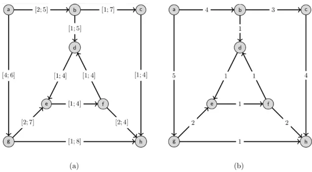
4.1 Examples of a RSPT instance (a) and one possible scenario (b) . . . 13
List of Tables
2.1 Smart environment application domains [Gubbi et al., 2013] . . . 5
6.1 Results for CPLEX Branch-and-bound Karaşan instances with 100 nodes . 27 6.2 Results for CPLEX Branch-and-bound for Karaşan instances with 200 nodes 27 6.3 Results for AM, AU and AMU for Karaşan instances with 100 nodes,
com-pared with the CPLEX branch-and-bound . . . 28 6.4 Results for AM, AU and AMU for Karaşan instances with 200 nodes,
com-pared with the CPLEX branch-and-bound . . . 28 6.5 Results for different versions of SBA . . . 29 6.6 Results for CPLEX branch-and-bound, AMU and two different SBAs for
Karaşan instances with 200 vertices . . . 30 6.7 Results for CPLEX branch-and-bound and MILP-VND for Karaşan
in-stances with 200 vertices . . . 31 6.8 Results for CPLEX Branch-and-bound and heuristics for Karaşan instances
Contents
Resumo ix
Abstract xi
List of Figures xiii
List of Tables xv
1 Introduction 1
2 Routing in 6LoWPAN 5
3 Related works 9
4 The Robust Shortest Path Tree 13
4.1 The problem . . . 13 4.1.1 RSPT complexity proof . . . 14 4.2 A mixed integer linear programming formulation . . . 17
5 Heuristics for RSPT 19
5.1 Proof of AM 2-approximation for RSPT . . . 20 5.2 MILP-based Variable Neighbourhood Descent . . . 22
6 Computational Experiments 25
6.1 CPLEX branch-and-bound . . . 26 6.2 Average Median Upper algorithm . . . 26 6.3 Scenario-based Algorithm . . . 29 6.4 Mixed Integer Linear Programming Variable Neighbourhood Descent . 31 6.5 Comparison of heuristics . . . 32
Bibliography 35
Chapter 1
Introduction
Nowadays, there is a steady growth in the number of Internet-connected devices such as computers, sensors, actuators, smartphones, home appliances, etc. [Atzori et al., 2010]. This new set of devices introduces a novel paradigm in the scenario of modern wireless telecommunications. These devices communicate with other and collaborate with their neighbours to reach common goals, forming the Internet of Things (IoT) [Giusto et al., 2010].
IoT refers to the networked interconnection of daily use objects, thus leading to a ubiquitous system. This ubiquity of the Internet is obtained by integrating objects via embedded systems. This leads to a highly distributed network of devices that communicate with each other and with people at their surrounding [Xia et al., 2012]. It can be characterized as a highly dynamic and distributed network system, composed of a large number of smart objects that produce and consume information [Miorandi et al., 2012].
A large number of applications are being developed for the IoT, with promises that this new paradigm will improve our quality of life [Xia et al., 2012]. However, many challenges, such as energy consumption, security and well designed routing protocols need to be solved before IoT becomes a reality. One of the most promising technolo-gies for the implementation of IoT is the IPv6 Low Wireless Personal Area Network (6LoWPAN) [Shelby and Bormann, 2011]. It is characterized by low resources in terms of both computation and energy capacity [Atzori et al., 2010; Gubbi et al., 2013]. Each 6LowPAN node represents a device in the IoT. These nodes are interconnected by wireless links with potentially low communication quality and high loss rates [Winter, 2012].
2 Chapter 1. Introduction
the IPv6 Routing Protocol for Low-Power and Lossy Networks (RPL) [Winter, 2012; Gaddour and Koubâa, 2013]. For each application running at the network, a sink node s is specified. Then, RPL builds a Destination Oriented Direct Acyclic Graph (DODAG) froms to all other nodes serving the application. The DOGAG represents all the possible routes from the sink to any other node in the application, and vice-versa. It is built taking into account the nodes’ transmission range and the distance between nodes. Each node may have one or more parent nodes, and the arcs are oriented from the node to its parents.
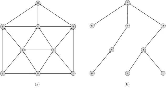
Once the DODAG is built, a default parent is selected for each node, which induce as-rooted tree that is a subgraph of the DODAG. This tree specifies the default routes between nodes in a 6LoWPAN, and its is referred to as the routing tree. It is computed taking into account a predefined metric regarding the link quality. There are an exponentially large number ofs-rooted trees in a DODAG, and the efficiency of the network depends on how good is the one chosen by the protocol. Therefore, each node periodically updates its parent, inducing a possibly better routing tree. An example of a DODAG and a routing tree is presented in Figure 1.1. In this example, the sink node isa, and a package from nodee to node f follows the path < e, c, a, d, f >.
(a) (b)
Figure 1.1. (a) An example of a DODAG rooted on nodea, and (b) an example
of a routing tree in this DODAG. In this example, a package from nodeeto node
f follows the path< e, c, a, d, f >
3
the performance of RPL may vary with the network links variability. The objective of this work is to improve the performance of RPL networks by taking into account link variability in the routing protocol.
Two main strategies can be used to optimize problems with data variability: stochastic programming [Spall, 2005] and robust optimization [Kouvelis and Yu, 1997; Ben-Tal and Nemirovski, 2002]. The former is mostly applied whenever the probability law associated to the uncertain data is known in advance. A drawback of this approach is that it is sometimes difficult to define the probability distribution associated to the uncertain data, or else errors can happen on the parameters estimation.
Robust optimization (RO) is an alternative to stochastic programming, where the variability at the uncertain data is represented by a set of deterministic values. The realization of the uncertain data, bounded by the determined interval, is called a scenario of a instance of a RO problem. RO is properly used when there is some uncertainly data that can be recovered from past times observation of the problem that will be optimized. A RO framework presented in [Kouvelis and Yu, 1997] defines three critical steps to build a robust model. Thefirst step is to structure the uncertain data. It defines that the uncertain data can be structured by a discrete set of scenarios, each one with a single value for each uncertain data, or by an interval of values for each uncertain parameter, which leads to an infinite number of scenarios. The second step is to choose an appropriate robust criterion, that determines how conservative will be the robust model. The last step is to gather the chosen data structure and robust criterion to build a robust model. Given the robust model, a solution is said to be robust if it has the smallest value for the robust criterion, among all feasible solutions. The robust optimization problem is defined as tofind the robust solution for a given robust model. There are three main robust criteria, namely the regret (RE) [Kouvelis and Yu, 1997; Karaşan et al., 2001], the minmax regret (MR) [Kouvelis and Yu, 1997; Aissi et al., 2009], and the minmax relative regret (RR) [Kouvelis and Yu, 1997; Coco et al., 2014a]. They are explained below.
Let R be the set of possible scenarios for a given problem, and X be the set of feasible solutions for this problem. Also, let xr be the cost of solutionxfor the scenario r. The RE criterion is defined as
min
4 Chapter 1. Introduction
Let R, X and xr be as defined above. Let also x∗
r be the cost of the optimal solution x∗
r for the scenario r. The MR criterion is defined as
min
x∈X maxr∈R{xr−x ∗
r}, (1.2)
i.e., the robust solution is one that minimizes the maximum regret over all scenarios. Analogously, the MRR creterion is defined as
min
x∈Xmaxr∈R �
xr−x∗ r x∗
r �
, (1.3)
i.e., the regret of using xr instead of x∗
r relative by the cost of xr [Kouvelis and Yu, 1997]. MRR is more difficult to solve, when compared to MR, because its objective function is nonlinear. However, MRR is a better metric than MR, as shown in [Coco et al., 2014a].
In this work, the RPL routing problem is modeled as a robust optimization prob-lem derived from the Shortest Path Tree probprob-lem (SPT) [Wu and Chao, 2004; Cormen et al., 2009]. Given a connected digraphG= (V, A)with a set V of nodes and a setA of arcs. Each arc (i, j)∈ A is associated with a cost cij ∈ R+. Moreover, let n =|V|
and m = |A| be respectively the number of nodes and arcs in G. SPT consists in finding a spanning tree of G that has the shortest path from a given root node s to every node inV \ {s}. There are polynomial time algorithms that solve the SPT, such as Dijkstra algorithm [Dijkstra, 1959] and Bellman-Ford algorithm [Bellman, 1956].
The Robust Shortest Path Tree problem (RSPT) is a generalization of SPT, where the cost of each arc(i, j)∈A is defined by an interval [lij, uij], withlij, uij ∈R+, such that uij ≥ lij >0,∀(i, j)∈ A. Also, let s∈ V be the root node. In our model for the RPL routing problem, the nodes inV are associated to IoT devices, and the arcs inE are associated to links. Besides, for all(i, j)∈A,lij anduij correspond to the smallest and the largest observation in the link quality metric. This problem is formally defined in Chapter 4.
Chapter 2
Routing in 6LoWPAN
Embedded devices (ED), also called smart objects, are a part of the Internet that consists in resource-constrained IP-enabled devices [Shelby and Bormann, 2011; Ee et al., 2010]. The IoT connects such devices, and will impact significantly in various sectors of the society, as environmental monitoring, energy savings, smart grids, more efficient factories, logistics, healthcare and smart homes [Atzori et al., 2010; Giusto et al., 2010; Xia et al., 2012; Shelby and Bormann, 2011; Gubbi et al., 2013; Kushalnagar et al., 2007; Kortuem et al., 2010; Said and Masud, 2013; Madakam et al., 2015].
smart smart smart smart
office/building city agriculture transportation
network size small medium medium/large large
# users not too many, general few, large, general
many public landowners public
energy battery battery, battery, battery,
harvesting harvesting harvesting
databases local shared local, shared shared
connectivity wifi/3G/4G/ wifi/3G/4G wifi/ wifi/
backbone backbone satellite satellite
bandwidth small large medium medium/large
examples Furdík and Lukác [2012] Zanella et al. [2014] TongKe [2013] Lee et al. [2015]
Table 2.1. Smart environment application domains [Gubbi et al., 2013]
6 Chapter 2. Routing in 6LoWPAN
of EDs connecting the public transportation, as presented by Lee et al. [2015]. This work focus on office/building networks, with low bandwidth and hundred of devices.
The network constructed by interconnected wireless EDs is a subset of the IoT, and is called Wireless Embedded Internet (WEI). The 6LoWPAN was developed to enable WEI to work with the IPv6 protocol, instead the traditional IPv4 protocol, thus enabling a vast amount of dispositives to be on the IoT [Shelby and Bormann, 2011].
The EDs communication devices typically benefit from multi-hop mesh networks, i.e. networks wherein messages are routed from a source to a destination through pos-sibly multiple other nodes acting as relays. A 6LoWPAN is a multi-hop mesh network, such that a path is formed by the set of links (i.e., channels) between the source and the destination. However, current IPv4 protocols may not easily be applicable to these networks, as discussed in [Shelby and Bormann, 2011].
Some protocols were designed for 6LoWPAN networks [Winter, 2012; Ee et al., 2010; Vasseur et al., 2011; Felsche et al., 2012]. One of the first protocols is the 6LoWPAN On-demand Distance Vector Routing (LOAD) [Kim et al., 2007b; Chang et al., 2010]. It is a simplified on-demand routing protocol based on Ad-Hoc On-demand distance vector routing (AODV) [Royer and Perkins, 1999; Perkins et al., 2003], that was first proposed for wireless sensor networks (WSN). Both LOAD and AODV use IEEE 64-bit address as devices interface identifiers for building it routing table. However, because of its length, the IEEE address is not scalable and inefficient when used in a 6LoWPAN network [Zhu et al., 2009].
The Dynamic MANET On-demand for 6LoWPAN Routing protocol (DYMO-low) [Kim et al., 2007a] is based on the Dynamic MANET On-demand Routing protocol (DYMO) [Chakeres and Perkins, 2008] and the AODV protocol. DYMO-low is a routing protocol for 6LoWPAN that works directly on the link layer, not using the network IP layer. Thus, it creates a mesh network topology of 6LoWPAN devices that do not have the knowledge of IP, such that IP sees this network as a single link, with all EDs sharing a same IPv6 prefix. This protocol is able to use both 16-bit link layer short address or IEEE 64-bit extended address.
7
The IPv6 Routing Protocol for Low-Power and Lossy Networks (RPL) [Vasseur et al., 2011; Winter, 2012; Gaddour and Koubâa, 2013] was designed to be highly adaptive to network conditions and to provide alternate routes, whenever default routes are inaccessible. RPL also works with 16 bits link layer short address, one of the characteristics of 6LoWPAN.
RPL is the most promising routing protocol for 6LoWPAN when compared to other protocols [Gaddour and Koubâa, 2013]. RPL is flexible, supporting various types of traffic (MP2P, P2MP and P2P). Thus, it can be easily adapted for various application requirements. It is also flexible and can use any metric to build its routing table. Besides, RPL is suitable for fault-tolerance applications, with a local and a global repair of its routing table [Gaddour and Koubâa, 2013].
RPL is based on the topological concept of a DODAG. It is possible to define a network by one or more of this DODAGs at the same time, thus being denominated a RPL instance. Furthermore, one network can run multiple RPL instances at the same time, such that each instance serves to an different application. Thus, one node can join one or more of these instances [Gaddour and Koubâa, 2013].
The RPL protocol is composed of three different ICMPv6 control messages: (i)
DIS (DODAG Information Solicitation); (ii)DIO (DODAG Information Object); (iii)
DAO (DODAG Destination Advertisement Object) [Winter, 2012]. These messages are used to exchange information about the DODAG topology.
A comparison between RPL and the others 6LoWPAN routing protocols can be found in [Gaddour and Koubâa, 2013]. It shows that RPL is a flexible protocol that can directly connect to the Internet by using the IPv6 protocol, supports various types of traffic, and can be easily adapted for various types of applications. Therefore, [Gaddour and Koubâa, 2013] concludes that RPL outperform others 6LoWPAN routing protocols. A detailed description of how RPL works can be found in [Vasseur et al., 2011; Winter, 2012].
Values of link quality are used to make routing decisions. However, the great link variability in 6LoWPANs can degrade the link throughput, as observed in Koksal et al. [2006]. If one link channel varies, it can disrupt the network and cause the whole network to lose performance, or even fail [Atzori et al., 2010; Shelby and Bormann, 2011; Koksal et al., 2006]. Besides, no current routing protocols in the literature consider channel variability.
8 Chapter 2. Routing in 6LoWPAN
When this occurs, the network will fail, it may even get disconnected. Besides that, a large amount of energy will be used in order to retransmit messages that were lost in the network. Thus, the network will be even more congested due the high quantity of retransmitted messages.
Chapter 3
Related works
Robust optimization problems were first studied in [Gupta and Rosenhead, 1968]. Many RO problems were introduced by Kouvelis and Yu [1997]. For instance, the Robust Assignment problem [Deí et al., 2006; Pereira and Averbakh, 2011], the Robust Shortest Path problem [Karaşan et al., 2001; Coco et al., 2014a, 2016], the Robust Minimum Spanning Tree Problem [Yaman et al., 2001; Kasperski et al., 2012], the Robust Knapsack problem [Yu, 1996; Monaci and Pferschy, 2013] and Robust Net-work Design problem [Gutiérrez et al., 1996; Ukkusuri et al., 2007]. More recently, RO versions of classical N P-Hard problems have also been studied, as the Robust Travelling Salesman problem [Montemanni et al., 2006; Candia-Véjar et al., 2011], the Robust Set Covering problem [Degel and Lutter, 2013; Coco et al., 2015], the Robust Scheduling Optimization problems [Daniels and Kouvelis, 1995; Wu et al., 2009], and the Robust Restricted Shortest Path problem [Assunção et al., 2014], among others. This work refers to the survey [Ben-Tal and Nemirovski, 2002] for other RO problems. It also presents the main results of RO applied to uncertain linear, conic quadratic and semidefinite programming until the time of its publication.
A survey about robust optimization criteria is presented by Coco et al. [2014b]. This work addresses RO problems with discrete scenarios. The three main minmax regret criteria are reviewed, so as α-robustness [Kalaıet al., 2012],bw-robustness [Roy, 2010], andpw-robustness [Gabrel et al., 2013]. It also presents two new robust criteria that can be applied to measure the robustness of both scenarios and interval data models.
10 Chapter 3. Related works
for a widely range of RO problems. The work of Chekuri et al. [2007] proves that a single-source version of the Robust Network Design problem isN P-Hard in undirected graphs. The complexity of the Robust Least-Squares problem have be discussed in [Ghaoui and Lebret, 1997]. The work [Aron and Hentenryck, 2004] prove that the Robust Minimal Spanning Tree problem is N P-Complete even in graphs when the edges cost are defined as binary values, settling the conjecture presented in [Kouvelis and Yu, 1997]. The work of Averbakh [2001] presents the first problem that is N P -Hard when there is a finite set of scenarios, but is polynomial time solvable when the uncertainty is represented by interval data.
The first MILP formulation for the Robust Shortest Path problem was given by Karaşan et al. [2001]. Besides, a pre-processing algorithm for the Robust Shortest Path problem was given in this same work. It consists in finding the so called weak arcs, i.e. arcs that never will be in the optimal solution of the problem. This algorithm is valid only for acyclic, planar or layered graphs. The idea of identifying weak arcs in a solution is extended to the Robust Travelling Salesman problem in [Montemanni et al., 2006, 2007].
A constraint programming approach to the Robust Minimal Spanning Tree prob-lem with interval data was developed by Aron and Hentenryck [2002]. The proposed search algorithm is based on three basic components: a combinatorial lower bound, a pruning component and a branching heuristic. Computational experiments show that the proposed algorithm outperforms the MILP based branch-and-bound algorithm pro-posed by Yaman et al. [2001].
Benders decomposition approaches for the Robust Shortest Path problem and the Robust Minimal Spanning Tree problem are presented by Montemanni and Gam-bardella [2005a] and Montemanni [2006], respectively. These works extend the pre-vious works of Montemanni et al. [2004] and Montemanni and Gambardella [2005a], that have presented branch-and-bound algorithms for these two problems. It is shown that the benders decomposition approach outperforms the previous branch-and-bound algorithms and all others state-of-the-art algorithms until the time of its publication.
The work of Kouvelis and Yu [1997] is extended in Averbakh [2005]. It considers the robust version of combinatorial optimization problems with discrete scenarios and the RR criterion. The author proposes a nonlinear generic formulation for this class of problem, and also developed a proof that RO problems with interval data with the RR criterion areN P-Hard.
11
then runs an algorithm for the classical version of the problem. This 2-approximative algorithm has the same complexity as the algorithm for the classical problem.
A polynomial time(1 +ε)-approximative scheme for RO problems is presented by Kasperski and Zieliński [2007], extending the work [Kasperski and Zieliński, 2006]. This algorithm can be applied for all RO problems that its classical version is polynomially solvable. Its complexity for the Robust Shortest Path problem is O(|A|3/ε2), where A
is the set of arcs of the problem.
Approximative algorithms for RO problems with interval data and AR criterion was developed in Conde [2012]. This work extends the previous work of Kasperski and Zieliński [2006, 2007]. It aims to solve the classical version of RO problems at the mean scenario, obtaining algorithms that have an approximation factor of 2 for minmax absolute regret problems [Kasperski and Zieliński, 2006, 2007].
Four pre-processing algorithms for Robust Shortest Path were developed by Catanzaro et al. [2011]. This work extends the work of Karaşan et al. [2001], by presenting new algorithms to fix arcs in the optimal solution. The first algorithm aims to find an subset of arcs that, if removed from the problem, result in solutions with a worst robustness cost. The second algorithm search for nodes that are not in any path between the origin node sand destination nodet. The third algorithm construct a Minimum Spanning Tree (MST) t at the upper scenario, i.e. a scenario where each arc of the graph is at it respective maximum value, and then find a shortest path p1
between s and t in t. Then, one arc(i, j)∈p1 is removed from the original graph and
a new shortest path p2 is evaluated at the resultant graph. If the robustness cost of
shortest path p1 is lower than shortest path p2, then the this arc (i, j) belongs to the
optimal solution of the problem. The last algorithm construct a MST t� at the lower scenario, i.e. a scenario where each arc of the graph is at it respective minimum value, and thenfind a shortest pathp�1 betweens andt int�. After that, an arc(i, j)∈G\t� is inserted in t�, and a new shortest path p�2 is evaluated in t�. If this new arc (i, j) do not belongs to the shortest path p�2, then it can be removed from the problem.
These four algorithms has complexity equals O(|V|2 × |A|), O(|V|3), O(|V|2 × |A|),
and O(|V|2× |A|), respectively, where V represents the set of nodes and A represents
the set of arcs of a graph G.
12 Chapter 3. Related works
reasonable running time. An extension of this work is presented in Coco et al. [2016], that develops hybrid algorithms that combine SBA and exact methods for this same problem.
Chapter 4
The Robust Shortest Path Tree
4.1
The problem
LetG= (V, A)be a connected digraph, whereV is the set of nodes andA is the set of arcs. Each arc (i, j)∈ A is associated with an interval cost [lij, uij], which represents the variation in the link quality metric, with lij, uij ∈R+ and uij ≥lij >0, for all arcs
(i, j)∈A. Let also s ∈V be the root node, andV� =V \ {s}.
Definition 4.1.1. A scenario r is a realization of arcs cost cr
ij ∈ [lij, uij] for each arc
(i, j)∈A.
(a) (b)
14 Chapter 4. The Robust Shortest Path Tree
Figure 4.1 shows an example of a RSPT instance and one possible scenario defined in this network. One can see that Figure 4.1b has a cost for each arc defined inside the interval cost presented in Figure 4.1a.
LetT be the set of all s-rooted spanning trees inG. Let alsopt
i be the path from nodes to nodei∈V� induced by the treet ∈T. Besides, letcr(pt
i) = �
(i,j)∈A[pt i]c
r ij be the cost ofpt
i in the scenario r, and cr(p∗i) be the cost in the scenarior of the shortest pathp∗
i from s toi inr.
Definition 4.1.2. The robust deviation of a path pt
i induced by t∈T in the scenario r(also referred to as theregret ofpt
i inr) is defined asdr(pti) =cr(pti)−cr(p∗i), i.e. the difference between the cost of pt
i in r and the best possible path from s toi in r.
LetA[t] be the set of arcs that compose a tree t∈T, andA[pt
i]⊂A[t] be the set of arcs that compose the pathpt
i, and R be the set of all possible scenarios in G.
Lemma 4.1.1. [Kouvelis and Yu, 1997] The robust deviation of pt
i is the maximum,
among all scenarios inR, at the scenariort
i ∈R, such thatc rt
i
ij = 1, for all(i, j)∈A[pti],
andcr t i
ij = 0, for all (i, j)∈A\A[pti].
The smaller is the robust deviation of pt
i, the better is this path for sending packets froms toi. Besides, the smaller is the value of drt
i(pt
i), the more robust is this path to variations in the link quality.
Definition 4.1.3. The robustness cost of t ∈ T is defined as Rt = � i∈V�d
rt i(pt
i), i.e. the sum of the maximum robust deviation of every path froms to any other node in G.
A smaller robustness cost implies that, when there is a great link variability, the network will be less affected. The smallest is robustness cost of the communication tree of a 6LoWPAN, the more efficient and the more reliable is the network.
Definition 4.1.4. A treet∗ ∈ T is said to be robust if it has the smallest robustness cost among all trees inT.
Therefore, RSPT can be defined as tofind a robust spanning tree of Grooted in s, i.e. t∗ =argmin
t∈T Rt.
4.1.1
RSPT complexity proof
4.1. The problem 15
1972] and the3-Partition Problem (3PT) [Garey and Johnson, 1979]. It is proved that, with only two different scenarios, the RSPT problem is N P-Complete, and with an indefined number of scenarios, the RSPT problem is strongly N P-Complete.
Definition 4.1.5. Given a finite set I, and a weight ai ≥ 0,∀i ∈ I, the objective of the 2-Partition Problem is to find two subsets of I, namely X and Y, such that �
i∈Xai = �
i∈I\Y ai and X ∩Y = ∅. Karp [1972] demonstrated that 2PT is N P -Complete even when |X|=|Y|= |I2|.
Definition 4.1.6. Given afinite setI of exactly3lelements, and a weight ai ≥0,∀i∈ I, the objective of the3-Partition Problem is tofind mdisjoint subsetss1, s2, . . . , sm ⊆
I such that s1 ∪s2 ∪. . .∪sm = I, and �k∈siak = B,∀si ∈ m. Garey and Johnson [1979] demonstrated that 3PT is strongly N P-Hard even when B
4 < ai <
B
2,∀ai ∈I.
It is possible to note that, when this inequality is satisfied, a solution for 3PT consists in exactly m=l triplets such that the sum of elements in each triplet isB.
Theorem 4.1.2. The RSPT problem is N P-Complete, even in layered graphs with only 3 layers and 2 scenarios.
Proof. The 2PT problem can be reducted to RSPT. Given a 2PT instance, it is possible to construct a corresponding RSPT instance in polynomial time.
Let I be a finite set with |I| = m elements. It is possible to build a digraph G= (V, A)partitionated into 3 disjunt subsets of vertices V =V0∪V1∪V2. Subset V0
contains only one vertice, denominated s. Subset V1 contains 2m vertices, and subset
V2 contains m vertices. Besides, it is possible to define three disjunt subsets of arcs
A = A0 ∪A1 ∪A2. Subset A0 contains 2m arcs, constructing an complete bipartite
digraph betwen subsets V0 and V1. Subset A1 contains m arcs, such that there is an
arc from each vertice vi ∈V1 to a vertice wi ∈V2, for all 0≤i < m. One can see that
this construction corresponds to a layered digraph with 3 layers of vertices.
A RSPT problem can be constructed with only two scenarios, namely r1 and r2.
The cost of arcs e∈A0 are fixed in0 under both scenarios. At scenarior1, the cost of each arc ei ∈A1 isfixed inai, and the cost of arcs e∈A2 isfixed in 0. At scenario r2,
the cost of each arc ei ∈A2 isfixed in ai, and the cost of arcs e∈A1 is fixed in 0.
Given the above construction, let t1 and t2 be two shortest paths trees (SPT) in
G with root at vertice s in scenarios r1 and r2, respectively. Note that t1 and t2 are
unique by construction. Besides, letXandY be two set of arcs such thatX =E\A[t2]
and Y = E\A[t1]. A 2PT of I exists if and only if Rt1 =Rt2 =
1 2
�
16 Chapter 4. The Robust Shortest Path Tree
that A[t1] = E0 ∪X and A[t2] = E0 ∪Y. Both t1 and t2 are optimal solutions for
the RSPT instance. To prove the "only if" part, assume that Rt∗ = 1
2
�
k∈Iak]. Let t1 and t2 be two SPT at scenarios r1 and r2, respectively. Moreover, letX and Y be
two subsets of arcs such that X = A\A[t2] and Y = A\t1. By the construction of
the network, it is clear that (A[t1]∩A[t2])\E0 =∅. Also, by the construction of the
network, it is clear thatRt1 =Rt2 = 12�
k∈Iak. Thus, it must be a 2PT ofI in subsets X and Y.
Theorem 4.1.3. The RSPT problem is stronglyN P-Complete for an unbounded num-ber of scenarios, even in layered graphs with only 3 layers.
Proof. The 3PT problem can be reducted to RSPT. Given a 3PT instance, it is possible to construct a corresponding RSPT instance in polynomial time.
Let I be a finite set with |I| = 3l elements. It is possible to build a digraph G= (V, A)partitionated into 3 disjunt subsets of vertices V =V0∪V1∪V2. Subset V0
contains only one vertice, denominateds. SubsetV1 contains(3l)2 vertices, and subset
V2 contains 3l vertices. Besides, it is possible to define l+ 1 disjoint subsets of arcs
A=A1∪A2∪. . .∪El∪Al+1. SubsetAl+1 contains(3l)2 arcs, constructing an complete
bipartite digraph betwen subsets V0 and V1. All others l subsets contain 3l arcs with
origin in verticesv3l+i ∈V1 and destiny at vertices wi ∈V2, for i∈{0,1, . . . ,3l}. One
can see that this construction corresponds to a layered digraph with 3 layers of vertices. A RSPT problem can be constructed with an unbounded number l of scenarios. The cost of arcs e ∈ Al+1 are fixed at 0 under all scenarios. For each scenario ri ∈
{0,1, . . . , l}, the cost of each arc e ∈ Ai is fixed in ai. Besides, the cost of each arc e∈A\Ai isfixed in 0.
Given the above construction, let T = {t1, t2, . . . , tl} be the set of SPT of G
with root at vertices inG on scenarios {r1, r2, . . . , rl}, respectively, such that A[ti] =
E0\�j∈l,j=� itj. Note that all SPT ∈T are unique by construction. A 3PT of I exists if and only if there is a RSPTt∗ of G with Rt
∗ =B. To prove the "if" part, suppose
there exists a 3PT of I into l disjoint subsets with �
k∈sm = B,∀m ∈ {1,2, . . . , l}. It is possible to construct a set {t1, t2, . . . , tl} of SPTs in G as mentioned above. By
the construction of the network, the robustness cost of all SPTs are the same, i.e. Rti =B,∀ti ∈ T. Thus, Rt∗ =minRti,∀ti ∈T, that, by definition, is equal to B. To
prove the "only if" part, assume that Rt∗ = B. By the construction of the network,
4.2. A mixed integer linear programming formulation 17
�
k∈Iak = lB. As there are l SPT in G with robustness cost equal to B, there is exactly a 3PT of I into subsets s1, s2, . . . , sl.
4.2
A mixed integer linear programming
formulation
A Mixed Integer Linear Programming (MILP) formulation is defined with decision variables zij ∈{0,1} such that zij = 1 if arc (i, j) ∈A belongs to the robust tree and zij = 0 otherwise. Moreover, auxiliary variables yk
ij ∈ {0,1} keep the path from s to k ∈V \ {s} induced by the tree defined by variableszij. Besides, variablesxk
i ≥0have the cost of the shortest path from s toi∈V \ {s} in the scenario induced by the path from s tok (defined by variables yk
ij). Therefore, the shortest path froms tok in this scenario is kept in xk
k. The corresponding MILP formulation is defined by Equations (4.1) to (4.9).
min � k∈V\{s}
�
(i,j)∈A
(uijyijk)−x k k
(4.1)
�
(j,l)∈A yk
jl− �
(i,j)∈A yk ij =
1, if j =s −1, if j =k
0, otherwise
, ∀j ∈V, k∈V \ {s} (4.2)
xkj ≤x k
i +lij + (uij−lij)y k
ij, ∀(i, j)∈A, k ∈V \ {s} (4.3)
yk
ij ≤zij, ∀(i, j)∈A, k∈V \ {s} (4.4)
�
(i,j)∈A
zij =n−1 (4.5)
xks = 0, k∈V (4.6)
xk
18 Chapter 4. The Robust Shortest Path Tree
zij ∈{0,1}, ∀(i, j)∈A (4.9)
Chapter 5
Heuristics for RSPT
Kasperski and Zieliński [2006] developed three heuristics for the Robust Shortest Path problem. They are called Average Median (AM), Average Upper (AU) and Average Median Upper (AMU). This work first extends the AM, AU, and AMU heuristics for the RSPT.
AM receives as input a graph G = (V, A), the lower bound lij, and the upper bound uij for each arc (i, j) ∈ A. Next, the scenario rm is fixed, where the cost of the arcs are set to their respective mean value, i.e. cm
ij = (lij +uij)/2. Then, the regret of the solution is computed by constructing two Shortest Path Tree (SPT) by the Dijkstra’s algorithm. The first evaluates the cost of the SPT in scenario rm. The second evaluates the cost of the SPT on the worst scenario, as stated at Lemma 4.1.1. Then, the regret is computed and returned. The asymptotic worst case complexity of this heuristic is the same as that of Dijkstra’s algorithm, i.e. O(|E|+|V| ·log(|V|)). This heuristic is a 2-approximative algorithm for Robust Shortest Path. A proof that it is also 2-approximative for RSPT is given in Session 5.1.
AU receives the same input as AM. Next, the scenarioru isfixed, where the cost of the arcs are in their respective maximum value, i.e. cu
ij = uij. Then, the regret is computed in the same way as in AM and returned. The asymptotic worst case complexity of this heuristic is the same complexity of as that of AM.
AMU runs AM and AU and then returns the best solution found by these heuris-tics. As AMU uses AM, its also a 2-approximation algorithm for the RSPT.
A Scenario-based Algorithm (SBA) for the Robust Set Covering problem was presented in Coco et al. [2015, 2016], and is extended here to RSPT. SBA is an extension of AMU, where target scenarios between the lower scenario (rl, a scenario where the cost of the arcs are set to their respective lower, i.e. cm
20 Chapter 5. Heuristics for RSPT
the final scenario β; and the step size γ. All parameters have real values into the interval [0,1]. Target scenarios are computed as α +δγ, for all δ ∈ {0, . . . , i} such that α+δγ ≤ β. Thus, SBA investigates β−α
γ different scenarios. One can see that
both mean scenariorm and upper scenario ru can be obtained with SBA. Thus, it can produce solutions at least as good as AMU and also holds an approximation ratio of at most 2 for the RSPT.
This work advances the literature by developing a new heuristic to solve the RSPT, denominated MILP-based Variable Neighbourhood Descent (MILP-VND), and it is presented in Section 5.2. MILP-VND is compared with AM, AU, AMU [Kasperski and Zieliński, 2006, 2007], SBA [Coco et al., 2015, 2016], and the MILP formulation (4.1)-(4.9) in Chapter 6.
5.1
Proof of AM 2-approximation for RSPT
Lemma 5.1.1. Kasperski and Zieliński [2006] Let t�
, t��
∈T be two trees rooted in s.
Then, the following inequality holds for all r∈R:
dr(pt� k)≥
�
(i,j)∈A[pt� k]\A[p
t�� k ]
uij+ �
(i,j)∈A[pt�� k ]\A[p
t� k]
lij, ∀k ∈V \ {s} (5.1)
Lemma 5.1.2. Kasperski and Zieliński [2006] Let t�
, t��
∈T be two trees rooted in s.
Then, the following inequality holds:
dr(pt� k)≤d
r(pt��
k )+ (5.2)
�
(i,j)∈A[pt� k]\A[p
t�� k ]
uij + �
(i,j)∈A[pt�� k ]\A[p
t� k]
lij, ∀k ∈V \ {s}
Theorem 5.1.3. The performance ratio of algorithm AM for the RSPT is at most 2.
Proof. Let t ∈ T be the tree given by AM algorithm. Also, for all k ∈ V \ {s}, let A[pt
k] be the set of arcs from vertex s to k in t. We will prove that, for all t ∈ T, �
k∈V\{s}d r(pt
k)≤2 �
k∈V\{s}d r(pt
5.1. Proof of AM 2-approximation for RSPT 21
�
k∈V\{s}
�
(i,j)∈A[pt k]\A[p
t k]
uij − �
(i,j)∈A[pt k]\A[p
t k]
lij
≥ (5.3)
�
k∈V\{s}
�
(i,j)∈A[pt k]\A[p
t k]
uij − �
(i,j)∈A[pt k]\A[p
t k]
lij
From inequality (5.2), we have
dr(pt k)≤d
r(pt k) +
�
(i,j)∈A[pt k]\A[p
t k]
uij + � (i,j)∈A[pt
k]\A[p t k]
lij, ∀k ∈V \ {s} (5.4)
We can rewrite inequality (5.4) as
�
k∈V\{s} dr(pt
k)≤ �
k∈V\{s} dr(pt
k)+ (5.5)
�
k∈V\{s}
�
(i,j)∈A[pt k]\A[p
t k]
uij + �
(i,j)∈A[pt k]\A[p
t k]
lij
Inequality (5.1) together with inequality (5.3) yield
dr(pt k)≥
�
(i,j)∈A[pt k]\A[p
t k]
uij − �
(i,j)∈A[pt k]\A[p
t k]
lij ≥ (5.6)
�
(i,j)∈A[pt k]\A[p
t k]
uij − �
(i,j)∈A[pt k]\A[p
t k]
22 Chapter 5. Heuristics for RSPT
�
k∈V\{s} dr(pt
k)≥ (5.7)
�
k∈V\{s}
�
(i,j)∈A[pt k]\A[p
t k]
uij − �
(i,j)∈A[pt k]\A[p
t k] lij ≥ �
k∈V\{s}
�
(i,j)∈A[pt k]\A[p
t k]
uij − �
(i,j)∈A[pt k]\A[p
t k]
lij
Inequalities (5.5) and (5.7) imply that �
k∈V\{s}d r(pt
k) ≤ 2 �
k∈V\{s}d r(pt
k) for anyt ∈T. Therefore, it is also valid for the robust tree, which completes the proof.
5.2
MILP-based Variable Neighbourhood Descent
The MILP-VND heuristic consists in a local search procedure that uses CPLEX to evaluate the neighbourhood of a solution. It implements a Variable Neighbourhood Descent [Talbi, 2009], a traditional local search metaheuristic that exploits the idea of neighbourhood change to escape from local optimum solutions [Hansen and Mladen-ović, 2001].
The MILP-VND uses the σ-opt neighbourhood structure [Lin, 1965], with σ ∈
{1, . . . ,4}. It receives as input a graph G = (V, A), besides the lower bound lij and the upper bound uij for each arc (i, j) ∈ A. Then, it runs SBA and use its solution as an initial point for the local search procedure. As MILP-VND starts from the SBA solution, it is also returns a solution that worst cost it at most twice of the optimal one.
The use of CPLEX for solving the neighbourhood structure instead of the tra-ditional enumeration strategy is justified by the complexity of verify the value of a neighbourhood. The evaluation of one solution consist in running two times the Dijk-stra’s algorithm, that is well-known to has the complexity of O(|A|+|V|log|V|). As MILP-VND uses up to a 4-opt neighbourhood structure, the complexity to verify a complete neighbourhood using the enumeration strategy is up toO(|A|+|V|log|V|)4.
Thus, using CPLEX can speed up the local search procedure.
5.2. MILP-based Variable Neighbourhood Descent 23
�
(i,j)∈t
zi,j =|V|−1−σ (5.8)
Chapter 6
Computational Experiments
Computational experiments were performed on an Intel Xeon CPU E5645 with 2.4
GHz clock and 32GB of RAM memory, running Linux operating system. The
branch-and-bound implementation of the ILOG CPLEX version 12.6 with default parameter
settings has been used to solve the MILP formulation (4.1)-(4.9). The heuristics have been implemented from scratch in C++ and compiled with GNU GCC version 5.2.1. The running time of CPLEX branch-and-bound was limited 24 hours.
The performance of AM, AU, AMU, SBA, and MILP-VND are assessed on a classic set of RSP instances, based on Karaşan graphs [Karaşan et al., 2001] with 100 and 200 nodes. Karaşan graphs rely on a layered [Sugiyama et al., 1981] and acyclic [Bondy and Murty, 1976] topology, see for example Figure 6.1. Instances are generated as in Coco et al. [2014a]. The instance names are presented as K-n-a-b-c-d, where n is the number of nodes and d is the graph width. Parameters a and b are used to generate the intervals [lij;uij]. For each arc (i, j) ∈ A, a value c ∈ [1;a]
26 Chapter 6. Computational Experiments
Figure 6.1. A Karaşan graph with M = m layers and width W = 2[Karaşan
et al., 2001]
6.1
CPLEX branch-and-bound
The first experiment aims at evaluating the performance of the CPLEX branch-and-bound based on the MILP formulation (4.1)-(4.9) for the proposed instances. Besides, these results are used to evaluate the proposed heuristics in comparison to CPLEX upper bound.
The results are reported in Tables 6.1 and 6.2. Thefirst column is the instances’ name. The second and third columns show the lower bound and the upper bound founds by CPLEX, respectively. The fourth column shows the relative optimality gap. The last column shows the running time in seconds. It can be seen that CPLEX branch-and-bound easily solve at optimality all the instances with 100 nodes, with an maximum running time of 7.55 seconds. However, for the instances with 200 nodes, the CPLEX branch-and-bound can only solve four out of the ten evaluated instances in less than 24 hours. However, the maximum optimality gap observed for this set of instances was 1.56%.
6.2
Average Median Upper algorithm
6.2. Average Median Upper algorithm 27
instance lb up gap (%) t (s)
K-100-200-0.9-a-2 22.00 22.00 0.00 0.72 K-100-200-0.9-b-2 83.00 83.00 0.00 0.80 K-100-200-0.9-a-5 228.00 228.00 0.00 2.74 K-100-200-0.9-b-5 370.00 370.00 0.00 4.58 K-100-200-0.9-a-10 39.00 39.00 0.00 4.07 K-100-200-0.9-b-10 27.00 27.00 0.00 4.16 K-100-200-0.9-a-25 14.00 14.00 0.00 2.73 K-100-200-0.9-b-25 32.00 32.00 0.00 7.55 K-100-200-0.9-a-50 14.00 14.00 0.00 2.52 K-100-200-0.9-b-50 9.00 9.00 0.00 2.50
average 0.00 3.23
Table 6.1. Results for CPLEX Branch-and-bound Karaşan instances with 100
nodes
instance lb up gap (%) t (s)
K-200-200-0.9-a-2 169,324.00 169,324.00 0.00 12,046.38 K-200-200-0.9-b-2 128,538.00 128,538,00 0.00 28,660.90 K-200-200-0.9-a-5 25,579.91 25,769.00 0.73 >86,000.00 K-200-200-0.9-b-5 15,383.15 15,390.00 0.04 >86,000.00 K-200-200-0.9-a-10 8,092.51 8,221.00 1.56 >86,000.00 K-200-200-0.9-b-10 6,979.42 7,086.00 1.51 >86,000.00 K-200-200-0.9-a-25 2,029.16 2,036.00 0.34 >86,000.00 K-200-200-0.9-b-25 2,363.35 2,382.00 0.80 >86,000.00 K-200-200-0.9-a-50 1,050.00 1,050.00 0.00 370.07 K-200-200-0.9-b-50 895.00 895.00 0.00 302.64
average 0.50 55,737.8
Table 6.2. Results for CPLEX Branch-and-bound for Karaşan instances with
200 nodes
28 Chapter 6. Computational Experiments
CPLEX AM AU AMU
instance gap (%) t (s) gap (%) t (s) gap (%) t (s) gap (%) t (s)
K-100-200-0.9-a-2 0.00 0.72 0.00 0.01 0.00 0.01 0.00 0.01
K-100-200-0.9-b-2 0.00 0.80 0.00 0.01 0.00 0.02 0.00 0.02
K-100-200-0.9-a-5 0.00 2.74 0.00 0.02 0.00 0.01 0.00 0.03
K-100-200-0.9-b-5 0.00 4.58 0.26 0.01 0.00 0.01 0.00 0.03
K-100-200-0.9-a-10 0.00 4.07 0.00 0.02 0.00 0.01 0.00 0.06
K-100-200-0.9-b-10 0.00 4.16 0.00 0.02 0.00 0.02 0.00 0.05
K-100-200-0.9-a-25 0.00 2.73 0.00 0.04 0.00 0.04 0.00 0.10
K-100-200-0.9-b-25 0.00 7.55 3.03 0.03 0.00 0.04 0.00 0.09
K-100-200-0.9-a-50 0.00 2.52 6.67 0.05 0.00 0.05 0.00 0.10
K-100-200-0.9-b-50 0.00 2.50 0.00 0.04 0.00 0.04 0.00 0.09
average 0.00 3.23 0.99 0.02 0.00 0.02 0.00 0.05
Table 6.3. Results for AM, AU and AMU for Karaşan instances with 100 nodes, compared with the CPLEX branch-and-bound
CPLEX AM AU AMU
instance gap (%) t (s) gap (%) t (s) gap (%) t (s) gap (%) t (s) K-200-200-0.9-a-2 0.00 12,046.38 0.01 0.02 0.01 0.02 0.01 0.07 K-200-200-0.9-b-2 0.00 28,660.90 0.69 0.02 0.69 0.02 0.69 0.06 K-200-200-0.9-a-5 0.73 >86,000.00 2.65 0.05 2.61 0.06 2.61 0.13 K-200-200-0.9-b-5 0.04 >86,000.00 2.08 0.02 2.08 0.02 2.08 0.05 K-200-200-0.9-a-10 1.56 >86,000.00 9.53 0.10 9.90 0.02 9.53 0.24 K-200-200-0.9-b-10 1.51 >86,000.00 6.74 0.10 4.17 0.12 4.17 0.24 K-200-200-0.9-a-25 0.34 >86,000.00 3.05 0.21 2.21 0.20 2.21 0.50 K-200-200-0.9-b-25 0.80 >86,000.00 4.13 0.22 3.94 0.22 3.94 0.48 K-200-200-0.9-a-50 0.00 370.07 2.86 0.31 2.23 0.34 2.23 0.72 K-200-200-0.9-b-50 0.00 302.64 4.48 0.34 4.58 0.38 4.48 0.78 average 0.50 55,737.80 3.62 0.13 3.24 0.14 3.19 0.33
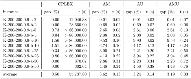
Table 6.4. Results for AM, AU and AMU for Karaşan instances with 200 nodes, compared with the CPLEX branch-and-bound
gap of 3.62%, while AU founds an relative gap of 3.24% and AMU achieves a relative gap of 3.19%. CPLEX branch-and-bound has a smaller gap of 0.50%, but an average running time of more than 55,000 seconds, while AM, AU and AMU running time never exceed 1 second.
6.3. Scenario-based Algorithm 29
6.3
Scenario-based Algorithm
The third experiment aims to evaluate SBA for the proposed instances. First, it presents a sensibility analysis of SBA in relation to its parameters. Then, SBA is compared with AMU and CPLEX branch-and-bound.
In order to evaluate the SBA sensibility to its parameters, 12 different versions of SBA were developed and evaluated. Three different sets of initial and final scenarios are considered, being {0,0.5},{0.5,1}, and {0,1}. Moreover, four different step sizes are considered, being 0.1,0.05,0.01, and 0.001.
As AMU solves all instances with 100 vertices at optimality, this experiment is performed only in instances with 200 vertices. Table 6.5 shows the results of the sensibility analisys of SBA. The first column shows the step size γ. The second and third columns show the initial scenario α and the final scenario β, respectively. The fourth column reports the number of inspected scenario by SBA with the definedα,β, andγ. Thefifth and sixth columns report, respectively, the average gap and the average running time over the proposed instances with 200 vertices for each combination ofα,β, and γ reported in columns 1, 2 and 3.
γ α β # scenarios gap (%) time (s)
0.1
0 0.5 6 2.67 0.97
0.5 1 6 2.80 0.81
0 1 11 2.48 1.55
0.05
0 0.5 11 2.59 1.55
0.5 1 11 2.68 1.55
0 1 21 2.41 2.98
0.01
0 0.5 51 1.87 7.25
0.5 1 51 1.99 7.27
0 1 101 1.73 14.28
0.001
0 0.5 501 1.75 69.86
0.5 1 501 1.94 68.90
0 1 1001 1.59 138.10
Table 6.5. Results for different versions of SBA
30 Chapter 6. Computational Experiments
applied to solve RSPT, a smaller average gap can be achieved when inspecting solutions between the lower scenario and the median scenario than between the median scenario and the upper scenario, for all step sizes. However, some instances have a smaller gap between the median scenario and the upper scenario. Thus, the best average gap is achieved when SBA inspect solutions between the lower scenario and the upper scenario, for all step sizes. The best evaluated set of parameters for SBA isα= 0,β = 1
andγ = 0.001, that achieved an average gap of only 1.59% in 138.10 seconds, in average.
Next, Table 6.6 reports the comparison of SBA with AMU and CPLEX branch-and-bound results presented in Tables 6.2 and 6.4. Two SBAs are analysed. Thefirst, called SBA1, have α = 0,β = 1 and γ = 0.01. The second, called SBA2, is the best evaluated SBA, as shown in Table 6.5. The first column reports the instances’ name. The second and third columns report CPLEX branch-and-bound gap and running time. Then, each pair of columns reffer to a heuristic. Thefirst column of each pair shows the relative gap of the solution found by the heuristic over the lower bound of the CPLEX branch-and-bound, in percentage. The second column of each pair shows the heuristic running time in seconds.
Table 6.6. Results for CPLEX branch-and-bound, AMU and two different SBAs
for Karaşan instances with 200 vertices
CPLEX AMU SBA1 SBA2
instance gap (%) t (s) gap (%) t (s) gap (%) t (s) gap (%) t (s)
K-200-200-0.9-a-2 0.00 12,046.38 0.01 0.07 0.01 2.60 0.00 23.43
K-200-200-0.9-b-2 0.00 28,660.90 0.69 0.06 0.69 2.62 0.68 23.65
K-200-200-0.9-a-5 0.73 >86,000.00 2.61 0.13 1.56 5.42 1.07 49.07
K-200-200-0.9-b-5 0.04 >86,000.00 2.08 0.05 1.18 5.32 0.86 51.23
K-200-200-0.9-a-10 1.56 >86,000.00 9.53 0.24 1.62 9.91 1.62 91.79
K-200-200-0.9-b-10 1.51 >86,000.00 4.17 0.24 1.91 10.09 1.68 97.24
K-200-200-0.9-a-25 0.34 >86,000.00 2.21 0.50 2.11 21.00 2.01 205.42
K-200-200-0.9-b-25 0.80 >86,000.00 3.94 0.48 2.23 21.02 2.23 200.66
K-200-200-0.9-a-50 0.00 370.07 2.23 0.72 2.23 31.04 2.23 308.39
K-200-200-0.9-b-50 0.00 302.64 4.48 0.78 3.58 33.67 3.35 330.14
average 0.50 55,737.80 3.19 0.33 1.71 14.28 0.95 138.10
6.4. Mixed Integer Linear Programming Variable Neighbourhood
Descent 31
6.4
Mixed Integer Linear Programming Variable
Neighbourhood Descent
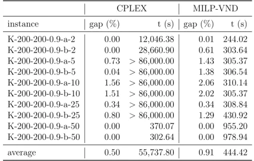
This experiment aims to evaluate MILP-VND for the proposed instances. As AMU solves all instances with 100 vertices at optimality, this experiment is performed only in instances with 200 vertices. The results of this experiment are shown in Table 6.7. The first column reports the instances’ name. The second and third columns report CPLEX branch-and-bound gap and running time. The fourth column shows the relative gap of the solution found by MILP-VND over the lower bound of the CPLEX branch-and-bound, in percentage. The last column reports the MILP-VND running time, in seconds.
Table 6.7. Results for CPLEX branch-and-bound and MILP-VND for Karaşan
instances with 200 vertices
CPLEX MILP-VND
instance gap (%) t (s) gap (%) t (s)
K-200-200-0.9-a-2 0.00 12,046.38 0.01 244.02 K-200-200-0.9-b-2 0.00 28,660.90 0.61 303.64 K-200-200-0.9-a-5 0.73 >86,000.00 1.43 305.37 K-200-200-0.9-b-5 0.04 >86,000.00 1.38 306.54 K-200-200-0.9-a-10 1.56 >86,000.00 2.06 310.14 K-200-200-0.9-b-10 1.51 >86,000.00 2.02 305.37 K-200-200-0.9-a-25 0.34 >86,000.00 0.34 308.84 K-200-200-0.9-b-25 0.80 >86,000.00 1.29 430.92 K-200-200-0.9-a-50 0.00 370.07 0.00 955.20 K-200-200-0.9-b-50 0.00 302.64 0.00 978.94
average 0.50 55,737.80 0.91 444.42
32 Chapter 6. Computational Experiments
6.5
Comparison of heuristics
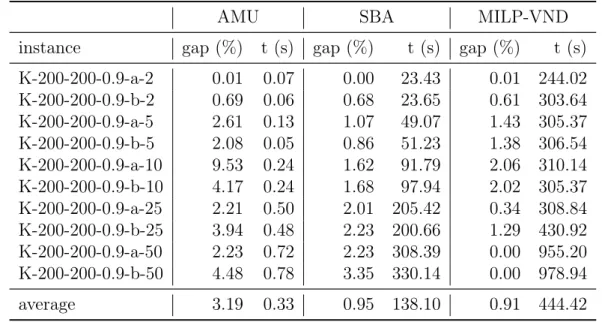
The last experiment compares the heuristics AMU, SBA, and MILP-VND with CPLEX branch-and-bound based on the proposed MILP formulation (4.1)-(4.9). The results of these experiments is shown in Table 6.8. First column represents the instance name. Next, each pair of consecutive columns refer to one heuristic, AMU, SBA, and MILP-VND, respectively. Thefirst column of each pair shows the relative gap of the solution found by the heuristic over the lower bound of the CPLEX branch-and-bound, in percentage. The second column of each pair shows the algorithm running time in seconds. As instances with 100 vertices are easily solved by CPLEX or AMU, Table 6.8 shows results only for instances with 200 vertices.
Table 6.8. Results for CPLEX Branch-and-bound and heuristics for Karaşan
instances with 200 nodes
AMU SBA MILP-VND
instance gap (%) t (s) gap (%) t (s) gap (%) t (s) K-200-200-0.9-a-2 0.01 0.07 0.00 23.43 0.01 244.02 K-200-200-0.9-b-2 0.69 0.06 0.68 23.65 0.61 303.64 K-200-200-0.9-a-5 2.61 0.13 1.07 49.07 1.43 305.37 K-200-200-0.9-b-5 2.08 0.05 0.86 51.23 1.38 306.54 K-200-200-0.9-a-10 9.53 0.24 1.62 91.79 2.06 310.14 K-200-200-0.9-b-10 4.17 0.24 1.68 97.94 2.02 305.37 K-200-200-0.9-a-25 2.21 0.50 2.01 205.42 0.34 308.84 K-200-200-0.9-b-25 3.94 0.48 2.23 200.66 1.29 430.92 K-200-200-0.9-a-50 2.23 0.72 2.23 308.39 0.00 955.20 K-200-200-0.9-b-50 4.48 0.78 3.35 330.14 0.00 978.94
average 3.19 0.33 0.95 138.10 0.91 444.42
Chapter 7
Conclusions
In this dissertation, the Robust Shortest Path Tree (RSPT) problem with interval data and minmax regret criteria was proposed. It was inspired by a real network application, the RPL routing problem. The RPL protocol builds a routing table for 6LoWPANs, that is a special type of network that composes the Internet of Things. This problem consists in computing a spanning tree in a given graph, such that the sum of the robust cost of the paths between the root node s and every other node of the network is minimized. In this work, the RSPT problem was formally defined, and a mathematical formulation was proposed. Besides, a set of algorithms for RSPT were presented and evaluated.
As far as we know, this is the first work in literature that develops optimization algorithms for the RPL protocol. Another novel contribution of this work is to use Robust Optimization techniques in order to consider the channel variability of 6LoW-PANs. Thus, this work proposes to extend the RPL protocol with the AU heuristic as objective function. As AU simple consists in running the Dijkstra’s algorithm in a pre-defined scenario, it can be implemented as a fully distributed network protocol.
To our knowledge, this is thefirst work in literature that deals with the RSPT. In order to compare the developed algorithms, a heuristic and three approximative algo-rithms for others Robust Optimization problems presented in [Kasperski and Zieliński, 2006] and [Coco et al., 2015] were extended for the RSPT. A proof that three of these algorithm holds a 2-approximation factor for the RSPT was developed. Besides, a Mixed Integer Linear Programming based local search was proposed. MILP-VND av-erage gap was just 0.41% greater than CPLEX branch-and-bound, but its running time was 2 orders of magnitude lower. Thus, it was considered the best heuristic to solve RSPT.
34 Chapter 7. Conclusions
Bibliography
Aissi, H., Bazgan, C., and Vanderpooten, D. (2009). Min-max and min-max regret versions of combinatorial optimization problems: A survey. European Journal of Operational Research, 197(2):427--438.
Aron, I. and Hentenryck, P. V. (2002). A constraint satisfaction approach to the robust spanning tree problem with interval data. In Proceedings of the Eighteenth Conference on Uncertainty in Artificial Intelligence, pages 18--25. Morgan Kaufmann Publishers Inc.
Aron, I. D. and Hentenryck, P. V. (2004). On the complexity of the robust spanning tree problem with interval data. Operations Research Letters, 32(1):36--40.
Assunção, L., de Noronha, T. F., Santos, A. C., and de Andrade, R. C. (2014). A lin-ear programming based heuristic for robust optimization problems: a case study on solving the restricted robust shortest path problem. InMatheuristics 2014-5th Inter-national Workshop on Model-Based Metaheuristics, Hambourg, Alemagne, page 8p.
Atzori, L., Iera, A., and Morabito, G. (2010). The Internet of Things: A survey.
Computer Networks, 54(15):2787–2805.
Averbakh, I. (2001). On the complexity of a class of combinatorial optimization prob-lems with uncertainty. Mathematical Programming, 90(2):263--272.
Averbakh, I. (2005). Computing and minimizing the relative regret in combinatorial optimization with interval data. Discrete Optimization, 2:273--287.
Bellman, R. (1956). On a routing problem. Technical report, DTIC Document.
Ben-Tal, A. and Nemirovski, A. (2002). Robust optimization–methodology and appli-cations. Mathematical Programming, 92(3):453--480.
36 Bibliography
Candia-Véjar, A., Álvarez-Miranda, E., and Maculan, N. (2011). Minmax regret com-binatorial optimization problems: an algorithmic perspective. RAIRO-Operation Research, 45:101--129.
Catanzaro, D., Labbé, M., and Salazar-Neumann, M. (2011). Reduction approaches for robust shortest path problems. Computers & Operations Research, 38:1610--1619.
Chakeres, I. and Perkins, C. (2008). Dynamic manet on-demand (dymo) routing. Technical report, Internet Engineering Task Force.
Chang, J. M., Yang, H. Y., Chao, H. C., and Chen, J.-L. (2010). Multipath design for 6lowpan ad hoc on-demand distance vector routing. International Journal of Information Technology, Communications and Convergence, 1(1):24--40.
Chekuri, C., Shepherd, F. B., Oriolo, G., and Scutellà, M. G. (2007). Hardness of robust network design. Networks, 50(1):50--54.
Coco, A. A., Júnior, J. C. A., Noronha, T. F., and Santos, A. C. (2014a). An integer linear programming formulation and heuristics for the minmax relative regret robust shortest path problem. Journal of Global Optimization, 60(2):265–287. ISSN 0925-5001.
Coco, A. A., Santos, A. C., and Noronha, T. F. (2015). Senario-based heuristics with path-relinking for the robust set covering problem. In Proceedings of the XI Metaheuristics International Conference (MIC).
Coco, A. A., Santos, A. C., and Noronha, T. F. (2016). Coupling scenario-based heuristics to exact methods for the robust weighted set covering problem with interval data. In VIII Conference on Manufacturing, Modelling, Management & Control.
Coco, A. A., Solano-Charris, E. L., Santos, A. C., Prins, C., and Noronha, T. F. (2014b). Robust optimization criteria: state-of-the-art and new issues. Technical report UTT-LOSI-14001, Université de Technologie de Troyes.
Conde, E. (2012). On a constant factor approximation for minmax regret problems using a symmetry point scenario.European Journal of Operational Research, 219:452--457.
Bibliography 37
Daniels, R. L. and Kouvelis, P. (1995). Robust scheduling to hedge against processing time uncertainty in single-stage production. Management Science, 41(2):363--376.
Degel, D. and Lutter, P. (2013). A robust formulation of the uncertain set covering problem. Working paper, Bochum.
Deí, V. G., Woeginger, G. J., et al. (2006). On the robust assignment problem under a fixed number of cost scenarios. Operations Research Letters, 34(2):175--179.
Dijkstra, E. W. (1959). A note on two problems in connexion with graphs. Numerische mathematik, 1(1):269–271.
Ee, G. K., Ng, C. K., Noordin, N. K., and Ali, B. M. (2010). A review of 6lowpan routing protocols. Proceedings of the Asia-Pacific Advanced Network, 30:71--81.
Felsche, M., Huhn, A., and Schwetlick, H. (2012). Routing protocols for 6lowpan. In
IT Revolutions, pages 71--83. Springer.
Furdík, K. and Lukác, G. (2012). Events processing and device interoperability in a smart office iot application. In Proceedings of the 23rd Central European Confer-ence on Information and Intelligent Systems (CECIIS 2012), University of Zagreb, Croatia, pages 387--394.
Gabrel, V., Murat, C., and Thièle, A. (2013). La pw-robustesse: pourquoi un nou-veau critère de robustesse et comment láppliquer? In 14eme congres de la Société Française de Recherche Opérationnelle et d’Aidea la Décision (ROADEF).
Gaddour, O. and Koubâa, A. (2013). Rpl in a nutshell: A survey. Computer Networks, 56(14):3163--3178.
Garey, M. R. and Johnson, D. S. (1979). Computers and Intractability: A Guide to
the Theory of NP-completeness. WH Freeman and Company, New York.
Ghaoui, L. E. and Lebret, H. (1997). Robust solutions to least-squares problems with uncertain data. SIAM Journal on Matrix Analysis and Applications, 18(4):1035--1064.
Giusto, D., Lera, A., Morabito, G., and Atzori, L. (2010). The Internet of Things. Springer.
38 Bibliography
Gupta, S. K. and Rosenhead, J. (1968). Robustness in sequential investment decisions.
Management science, 15(2):B--18.
Gutiérrez, G. J., Kouvelis, P., and Kurawarwala, A. A. (1996). A robustness approach to uncapacitated network design problems. European Journal of Operational Re-search, 94(2):362--376.
Hansen, P. and Mladenović, N. (2001). Variable neighborhood search: Principles and applications. European journal of operational research, 130(3):449--467.
Kalaı, R., Lamboray, C., and Vanderpooten, D. (2012). Lexicographic α-robustness: An alternative to min–max criteria. European Journal of Operational Research, 220(3):722--728.
Karaşan, O. E., Yaman, H., and Pinar, M. C. (2001). The robust shortest path problem with interval data. Technical report, Bilkent University, Department of Industrial Engineering.
Karp, R. M. (1972). Reducibility among combinatorial problems. In Complexity of computer computations, pages 85--103. Springer.
Kasperski, A., Makuchowski, M., and Zieliński, P. (2012). A tabu search algorithm for the minmax regret minimum spanning tree problem with interval data. Journal of Heuristics, 18(4):593--625.
Kasperski, A. and Zieliński, P. (2006). An approximation algorithm for interval data minmax regret combinatorial optimization problems.Information Processing Letters, 97(5):177--180.
Kasperski, A. and Zieliński, P. (2007). On the existence of an fptas for minmax regret combinatorial optimization problems with interval data.Operations Research Letters, 35(4):525--532.
Kim, K., Montenegro, G., Park, S., Chakeres, I., and Perkins, C. (2007a). Dynamic manet on-demand for 6lowpan (dymo-low) routing. Technical report, Internet Engi-neering Task Force.
![Table 2.1. Smart environment application domains [Gubbi et al., 2013]](https://thumb-eu.123doks.com/thumbv2/123dok_br/15587464.607462/23.892.135.776.671.924/table-smart-environment-application-domains-gubbi-al.webp)
![Figure 6.1. A Karaşan graph with M = m layers and width W = 2 [Karaşan et al., 2001]](https://thumb-eu.123doks.com/thumbv2/123dok_br/15587464.607462/44.892.150.729.143.334/figure-karaşan-graph-with-layers-and-width-karaşan.webp)