AN ALTERNATIVE EXPERIMENTAL METHOD TO DISCRIMINATE MAGNETIC PHASES USING IRM
ACQUISITION CURVES AND MAGNETIC DEMAGNETISATION BY ALTERNATING FIELD
Marcos A.E. Chaparro
1and Ana M. Sinito
2Recebido em 04 fevereiro, 2004 / Aceito em 23 julho, 2004 Received February 04, 2004 / Accepted July 23, 2004
ABSTRACT.Separation of different magnetic phases in natural samples composed by a mix of several magnetic minerals become necessary in rock magnetism in order to identify and describe the main magnetic carriers. However, this task may be difficult to carry out successfully.
The goal of the proposed method in this paper is to determine and discriminateexperimentallymagnetic (soft and hard) phases in synthetic and natural samples. The present method uses two different magnetic techniques, isothermal remanent magnetisation acquisition and magnetic demagnetisation alternately. After the entire process of induced remanent magnetisation and demagnetisation is performed, three residual isothermal remanent magnetisation curves are obtained. This discrimination is achieved by using asfilters (sorter)different peak values for alternating demagnetising fields.
Well-known pure and mixed synthetic iron oxides (magnetite and hematite) were firstly studied to investigate and corroborate the reliability of our experimental method, obtaining successful results. Subsequently, natural samples containing soft and hard minerals (magnetite, hematite, goethite, etc.) from stream-sediments, soils and a mine were also studied.
Comparisons with other purely numerical methods were carried out, yielding a good agreement among them. Our method is more time-consuming than others, but separation of individual magnetic curves is achieved by an experimental procedure, which is more realistic. It is also possible to apply this method to backfield isothermal remanent magnetisation measurements obtaining valuable information of HCRand S-ratio for each phase.
Keywords: Magnetic phases discrimination, Isothermal Remanent Magnetisation, Magnetic demagnetisation by AF, remanence coercivity, synthetic iron oxides.
RESUMEN.La separaci´on de distintas fases magn´eticas en muestras naturales, compuestas por diferentes minerales magn´eticos, se ha vuelto necesaria en magne-tismo a fin de identificar y describir los principales portadores. Sin embargo, esta tarea puede ser dif´ıcil de llevar a cabo.
El objetivo del m´etodo propuesto es determinar y discriminaren forma experimentalfases magn´eticas en muestras sint´eticas y naturales. El m´etodo usa dos t´ecnicas magn´eticas diferentes en forma alternada, adquisici´on de magnetizaci´on remanente isot´ermica y desmagnetizaci´on magn´etica. Una vez concluido el proceso de medici-ones de magnetizaci´on remanente inducida y desmagnetizaci´on magn´etica, usando comofiltro (clasificador)diferentes valores pico de campo alterno para la desmag-netizaci´on magn´etica, se obtienen tres curvas de magdesmag-netizaci´on remanente residual. Es tambi´en posible aplicar este m´etodo a mediciones de magdesmag-netizaci´on remanente isot´ermica de campo reverso obteniendo informaci´on valiosa de los par´ametros HCRy S-ratio para cada fase.
Oxidos de hierro sint´eticos puros y mezclados (magnetita y hematita) fueron primeramente estudiados para investigar y corroborar la confiabilidad de nuestro m ´etodo experimental, obteniendo los resultados esperados. En segundo t´ermino, se estudiaron muestras naturales conteniendo distintos minerales (hematita, goethita, magne-tita, etc.).
Finalmente, se llevaron a cabo comparaciones con otros m´etodos puramente num´ericos, obteniendo un buen acuerdo con ellos. Nuestro m´etodo es m´as costoso en tiempo, no obstante, la separaci´on es lograda por medio de un procedimiento experimental, el cual es m´as realista.
Palabras-clave: Discriminaci´on de fases magn´eticas, magnetizaci´on remanente isot´ermica, desmagnetizaci´on magn´etica usando AF, coercitividad de remanencia, ´oxidos de hierro sint´eticos.
1IFAS, Universidad Nacional del Centro de la Provincia de Buenos Aires, Pinto 399, 7000 Tandil, Argentina – Tel: +54 2293 444432, Fax: +54 2293 444433 – E-mail: [email protected]
INTRODUCTION
Isothermal Remanent Magnetisation (IRM) acquisition is very sensitive to the presence of diverse assemblages of magnetic grains; however, it is difficult to distinguish different magnetic phases from a natural sample composed by a mix of several mag-netic minerals.
The most popular methods to separate the magnetic compo-nent use the gradient of experimental IRM curve (e.g. Robertson and France, 1994; Stockhausen, 1998; Kruiver et al., 2001a and 2001b, Heslop et al., 2002). It is possible to model the IRM curve, although often there is more than one possible solution. If this is the case, additional background information is needed to remove the non-uniqueness and to obtain correct interpretations. Other methods for discriminating magnetic mineralogy, based on para-meters related to IRM acquisition (SIRM and remanent coercivity), are plots of Thompson and Oldfield (1986), biplots of Peters and Thompson (1998), flowcharts of Maher et al. (1999) and biplots of Peters et al. (2002).
Magnetic parameters derived from IRM acquisition measure-ments are closely influenced by predominant magnetic carriers. The influence and features of non-predominant magnetic carriers to bulk response can be mashed by the dominant ones and there-fore they cannot always be differentiated.
In this paper, an experimental method to find and discriminate various magnetic phases is proposed. The main tools used in this method are IRM acquisition and magnetic demagnetisation tech-niques. Parameters and curves obtained from these techniques are related to grain size and mineralogy of magnetic carriers, so both measurements can be jointly used to find out several mag-netic phases.
The main aim of this tool is to provide an experimental and therefore realistic discrimination of magnetic phases.
SAMPLES
Synthetic and natural samples
We study synthetic and natural materials. Synthetic iron oxides of magnetite (Fe3O4) and hematite (Fe2O3) from Bayferrox,
la-belled MgSth2 and HmSth respectively, were prepared and their magnetic properties were investigated in the laboratory. The mag-netite is a black powder and according to electron micrographs, its particles are spherical and the maximum grain size is0.2µm.
In the case of hematite, it is a red powder, its particles are acicular and the maximum grain size is0.1×0.8µm.
According to the BayferroxCompany, synthetic magnetite
contains approximately 90% of Fe3O4; synthetic hematite
con-tains between 97 and 98% of Fe2O3. Minute traces of ferrimag-netic materials were detected in our IRM preliminary studies of pure hematite (item 4, Fig. 3); thermal studies confirmed this re-sult. This ferrimagnetic phase was also detected in synthetic he-matites in other studies (de Boer and Dekkers, 1998; France and Oldfield, 2000). The material was thermally treated in order to re-move (minimise) the ferrimagnetic phase (possibly magnetite or maghemite) without affecting the hematite; it was heated in air up to750◦C. After this process, a new sample, HmSth3, was pre-pared by using the treated material. Two other samples were also prepared mixing different proportions of thermally treated hema-tite and magnehema-tite: HmMgSth1, 420 parts of hemahema-tite per one part of magnetite (420:1) and HmMgSth2, 110 parts of hematite per one part of magnetite (110:1).
The natural samples were collected from different environ-ments. Two samples (PE1a8 and PE1a12) were obtained from stream-sediments (La Plata, Argentina), belonging to different depths and therefore with different magnetic characteristics. One sample (GoP2) belongs to a soil from La Plata (Argentina), and the other sample of natural goethite (Goeth1b) was taken out from Tharsis (Spain). Exhaustive analysis on these samples were car-ried out by Chaparro et al. (2002a, 2002b and 2003).
THE METHOD
The method is based on the responses of different assemblages of magnetic materials when they are subject to a pulse magne-tising field and a demagnemagne-tising AF. From both studies, useful curves and magnetic parameters are achieved and therefore bulk data about magnetic carriers can be obtained, although only qua-litativeinformation of individual magnetic population can be in-ferred. However, numerical methods applied to IRM acquisition curves (Kruiver et al, 2001a; Heslop et al., 2002) have been suc-cessful developed in order to get a quantitative separation of bulk IRM curve into individual IRM contributing curves.
In this work an alternative method is proposed in order to split
0 20 40 60 80 100 0,0
0,2 0,4 0,6 0,8
N
o
rm
a
lis
e
d
R
e
m
a
n
e
n
t
M
a
g
n
e
ti
s
a
ti
o
n
Field (mT)
MgSth2 MDF
IRM= 11.54 mT
HmSth3 MDF
IRM= no
HmMgSth1 MDFIRM= no
HmMgSth2 MDF
IRM= 19.68 mT
0 20 40 60 80 100
0.0 0.2 0.4 0.6 0.8
N
o
rm
a
lis
e
d
R
e
m
a
n
e
n
t
M
a
g
n
e
tis
a
tio
n
Field (mT)
PE1a8 MDFIRM= 15.73 mT
PE1a12 MDFIRM= 44.57 mT
GoP2 MDFIRM= 38.85 mT
Goeth1b MDFIRM= no
Figure 1– Demagnetisation of SIRM curves for Synthetic (MgSth2, HmSth3, HmMgSth1 and HmMgSth2) and Natural samples (PE1a8, PE1a12, GoP2 and Goeth1b). Figura 1–Curvas de demagnetizaci´on de MRIS de muestras sint´eticas (MgSth2, HmSth3, HmMgSth1 y HmMgSth2) y naturales (PE1a8, PE1a12, GoP2 y Goeth1b).
10 100 1000
0 500 1000 1500
10 100 1000
IRM102.5[#16] TotalIRM[#27]
IRM50[#21]-IRM102.5[#21] TotalIRM[#19]-IRM50[#19] TotalIRM
IRM50
IRM102.5 Total[#27]
Phase3[#16]
Phase2[#21] Phase1[#19]
IR
M
(
m
A
m
-1)
Field (mT)
Figure 2– Total and Phases IRM acquisition curves obtained from equations 1a-c. (Inset) measured data points, TotalIRM measurements, and residual remanent magnetisation measurements (IRM50 and IRM102.5) are shown. Differences between measured remanent magnetisation (e.g. TotalIRM[#19]-IRM50[#19]) for two growing DC field steps (#19 and #21) and their corresponding results (e.g. Phase1[#19]) are shown. The direct relation between Total and Phase3 and TotalIRM and IRM102.5 curves is also shown, e.g. Phase3[#16]=IRM102.5[#16].
Figura 2–Curvas de MRI de adquisici´on Totales y Fases obtenidas de las ecuaciones 1a-c. En el recuadro, se muestran los puntos medido, mediciones de MRITotal, y mediciones de magnetizaci´on remanente residual (MRI50 y MRI102.5). Pueden apreciarse en el gr´afico las diferencias entre magnetizaciones remanentes medidas (por ej.: MRITotal[#19] - MRI50[#19]) para dos etapas de campo DC creciente (#19 y #21) y sus correspondientes resultados (por ej.: Fase1[#19]). Se muestra tambi´en, la relaci´on directa entre las curvas Total y Fase3, con MRITotal y MRI102.5 (por ej.: Fase3[#16] = MRI102.5[#16]).
Residual remanent magnetisation curves and discrimi-nation of IRM phase curves
Under low fields (AF∼50 mT) magnetic assemblages with pre-dominance of soft materials are almost completely demagnetised; on the other hand, harder materials do not show significant decre-ase of the remanent magnetisation (e.g. Dankers, 1978; Dankers, 1981; Bailey and Dunlop, 1983; Xu and Dunlop, 1995; Argyle et al., 1994; Dunlop and ¨Ozdemir, 1997). Dankers (1978) carried
in most cases, not significantly affected by higher AF (100 mT). However, it must be taken into account that remanent magnetisa-tion is partially reduced, in some cases up to 20% or more accor-ding to the kind of hematite and its grain size.
This fact can be useful if it is used as afilter (sorter)method between soft and hard magnetic phases. In this work we chose two peaks AF asAF filters, which were set at 50 mT (moderate filter) and 102.5 mT (relatively strong filter) with the aim of discri-minating material with different coercive forces.
Each sample was magnetised using a pulse magnetiser mo-del IM-10-30 ASC Scientific in 27 growing DC field steps (from 4.3 to 2470 mT) and three measurements were taken in each step with a spinner fluxgate magnetometer Minispin, Molspin Ltd. Af-ter each magnetisation step, remanent magnetisation (Total IRM (#i), i indicates the magnetisation step) was measured. The sam-ple was then demagnetised using 50 mT as peak value and its re-sidual remanent magnetisation was measured (named IRM50 (#i), i indicates the magnetisation step). Magnetic demagnetisation by thetumbling methodwas carried out using the Shielded Demag-netiser Molspin Ltd.Reversing optionwas chosen, allowing the direction of tumbling to be reversed every four rotations, and a decay rate of the peak AF of17µT per cycle was set. Finally, the
sample was demagnetised using a higher peak value (102.5 mT) and the new residual remanent magnetisation was measured (na-med IRM102.5 (#i) i indicates the magnetisation step). This pro-cess was carried out until saturation (i = 1 to 27, DC field for the 27thstep is 2470 mT) was reached (Saturation IRM, SIRM). At sa-turation three remanent magnetisations were measured; they are IRM(#27), named Total SIRM; IRM50(#27), named SIRM50; and IRM102,5(#27), named SIRM102.5. Total IRM curves and IRM for three different magnetic phases obtained by subtraction may be drawn,
P hase3(#1)=I R M102.5(#i) (1a)
P hase2(#1)=I R M50(#i)−I R M102.5(#i) (1b)
P hase1(#1)=T ot al I R M(#i)−I R M50(#i) (1c)
Residual remanent magnetisation, Total and Phase curves are shown on Fig. 2; differences between residual curves at two diffe-rent field steps (i = 19 and i = 21) and their corresponding results (data point from Phase1(#19), Phase1(#21) and Phase2(#19), Phase2(#21)) are also shown.
Phase 1 is the softest one(AF<50mT), Phase 2 is median (50mT < AF < 102.5mT)and Phase 3 is the hardest one
(AF>102.5mT). From this discrimination it is possible to find
every Phase SIRM and its corresponding magnetic contribution (%) to the Total SIRM. These percentages represent the contribu-tion to the remanent magnetisacontribu-tion (magnetic signal) and they are not (necessarily) directly related to the concentration of
magne-tic materials because all minerals (magnetite, hematite, goethite, etc.) also depend on magnetic features.
This method can also be applied to backfield measurements, although this process must be carried out separately for each demagnetising peak AF value. From Total SIRM, SIRM50 and SIRM102.5 backfield measurements are obtained. A residual backfield IRM curve is entirely achieved using only a determined peak AF value; after the process is finished another residual back-field IRM curve using another peak AF value is measured.
Finally, several magnetic parameters, remanent coercitivity (HCR), remanent acquisition coercitivity (H1/2), and S-ratio ((1-IRM-300mT/SIRM)/2, according to Bloemendal et al., 1992) from this magnetic discrimination can be estimated. From demagneti-sation curves the median destructive fields (MDF) were calculated.
MEASUREMENTS AND RESULTS
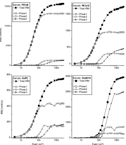
Total IRM measurements and the three Phases obtained for the different magnetic phases are displayed for each sample in Fig. 3, 4 and 5. Measured and calculated values for several related IRM parameters are listed in Tables 1 and 2.
10 100 1000
0 4000 8000 12000 16000
IR
M
(mA
/m
)
Field (mT) Sample: HmSth
Total IRM
Phase1 Phase2 Phase3
Figure 3– Total and Phases IRM acquisition for thermally untreated synthetic hematite, HmSth sample.
Figura 3–Curvas de MRI de adquisici´on Total y Fases para hematita sin tratar t´ermicamente, muestra HmSth.
As it was mentioned in item 2.1, preliminary studies of IRM acquisition for synthetic samples were carried out to test their magnetic properties. In the HmSth sample a high SIRM was ob-served; this Total SIRM is dominated by a soft phase, although a reduced hard phase is also present (Table 1 and Fig. 3).
10 100 1000
0 6000 12000 18000 24000
10 100 1000
0 1000 2000 3000 4000
10 100 1000
0 2000 4000 6000
10 100 1000
0 2000 4000 6000
IR
M
(
m
A
/m
)
Sample: MgSth2
Total IRM
Phase1 Phase2
S ample : HmSth3
Total IRM
Phase1 Phase2 Phase3
IR
M
(
m
A
/m
)
Field (mT)
Sample: HmMgSth1
Total IRM
Phase 1 Phase 2 Phase 3
Field (mT)
Sample: HmMgSth2
Total IRM
Phase1 Phase2 Phase3
Figure 4– Total and Phases IRM acquisition for synthetic samples. ”Pure”samples are MgSth2 (magnetite) and HmSth3 (thermal treated hematite); mixed samples are HmMgSth1 (420 parts of hematite per 1 of magnetite) and HmMgSth2 (110 parts of hematite per 1 of magnetite)
Figura 4–Curvas de MRI de adquisici´on Total y Fases para las muestra sint´eticas. Las muestras ”puras”son MgSth2 (magnetita) y HmSth3 (hematita t´ermicamente tratada); las muestras mezcla son HmMgSth1 (420 partes de hematita por 1 de magnetita) y HmMgSth2 (110 partes de hematita por 1 de magnetita).
Total SIRM (and specific SIRM) of the two stream-sediment samples (PE1a8 and PE1a12) are very different. GoP2 and Go-eth1b samples also showed differences (Table 2 and Fig. 5).
H1/2was calculated from Total IRM acquisition curves. High H1/2were found for synthetic samples with high content of hard materials (HmSth3 and HmMgSth1), and low H1/2for the other synthetic samples (MgSth2 and HmMgSth2) (Table 1). For
na-tural samples, the lowest value belonged to PE1a8 sample and similar H1/2was found for PE1a12 and GoP2. On the other hand, the highest H1/2was found for Goeth1b sample (Table 2).
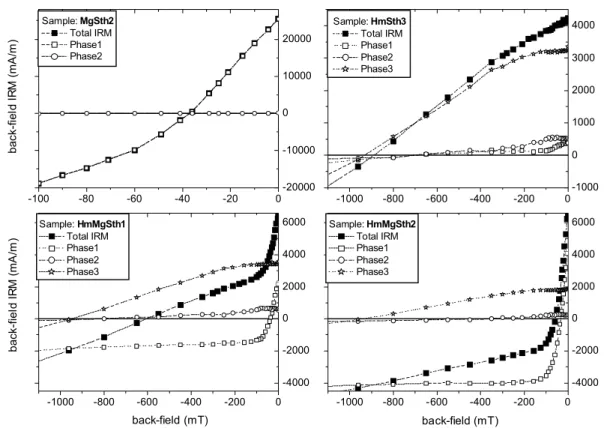
From backfield, HCRwere estimated (Fig. 6 and 7). They were in agreement with H1/2results for synthetic and natural samples as it can be observed in Tables 1 and 2.
10 100 1000
0 5000 10000 15000
10 100 1000
0 50 0 1000 1500
10 100 1000
0 200 400 600 800
10 100 1000
0 1000 2000 3000 4000
IR
M
(
m
A
/m
)
Sample: PE1a8 Total IRM Phase1 Phase2 Phase3
Sample: PE1a12 Total IRM Phase 1 Phase 2 Phase 3
IR
M
(
m
A
/m
)
Field (mT) Sample: GoP2
Total IRM Phase 1 Phase 2 Phase 3
Field (mT) Sample: Goeth1b
Total IRM Phase1 Phase2 Phase3
Figure 5– Total and Phases IRM acquisition for natural samples. PE1a8 and PE1a12 were obtained from stream-sediments, GoP2 belongs to a soil, and Goeth1b is a sample of natural goethite.
Figura 5–Curvas de MRI de adquisici´on Total y Fases para las muestra naturales. Las muestras PE1a8 y PE1a12 fueron extra´ıdas de sedimentos arroyo, la muestra GOP2 pertenece a un suelo, y Goeth1b es una muestra de goethita natural.
samples, the highest value corresponds to MgSth2, and lower values were found for the other synthetic samples (Table 1). The highest value for natural samples corresponds to PE1a8 and Go-eth1b sample has the lowest value (Table 2).
After demagnetisation with different peak AF values was ap-plied, equations (1a-c) were used in order to calculate the three magnetic phases for each sample and their corresponding mag-netic parameters (Fig. 4 and 5, Tables 1 and 2).
After IRM studies were done, additional measurements of demagnetisation of SIRM were made. Well-defined differences among demagnetisation curves and MDF parameter (MDFIRM) are observed in Fig. 2. MDFIRMwas calculated from these curves and corresponding results are summarised in Tables 1 and 2. Extreme
cases are MgSth2 (magnetite) and HmSth3 (hematite) synthetic samples, and PE1a8 (high content of natural magnetite) and Go-eth1b (natural goethite) natural samples. The MDFIRMwas not re-ached for samples with high contents of hard magnetic materials (like as hematite and goethite), HmSth3, HmMgSth1 and Goeth1b samples.
DISCUSSION
Synthetic samples, pure and mixed iron oxides
Table 1. Several magnetic parameters from IRM acquisition, magnetic demagnetisation and the proposed method for synthetic samples.
Tabla 1.Distintos parámetros magnéticos derivados de la MRI de adquisición, demagnetización magnética y el método propuesto para muestras sintéticas.
Magnetic Parameters Sample Magnetic
Phase
Contribution (%)
SIRM (mA/m)
SIRM (Am2
kg-1 )
HCR
(mT)
H1/2
(mT)
HCR/H1/2
(dimensionless)
S-ratio (dimensionless)
MDFIRM
(mT)
Total 100 26220 4.449 37.0 77.0 0.48 1.00 11.5
1 99.4 26052 37.0 76.6 0.50 1.00
MgSth2 (“Pure” synthetic
magnetite)
2 0.6 166 80.8 129.6 0.62 1.06
Total 100 4190 2.966E-2 889.5 992.1 0.90 0.14 --
1 5.1 217 702.7 546.6 -- 0.39
2 5.2 220 699.4 437.4 -- 0.30
HmSth3 (“Pure” synthetic
hematite)
3 89.7 3757 931.9 1083.4 0.86 0.30
Total 100 15747 8.360E-2 -- 50.6 -- -- --
1 89.2 14041 -- 46.7 -- --
2 1.2 189 -- 353.0 -- --
HmSth (Thermally untreated synthetic
hematite)
3 9.6 1517 -- 1099.1 -- --
Total 100 6474 3.928E-2 605.5 737.0 0.82 0.38 --
1 32.6 2115 37.9 58.9 0.61 0.85
2 3.4 223 829.2 391.2 -- 0.30
HmMgSth1 (Synthetic hematite
and magnetite 420:1)
3 64.0 4146 949.0 1091.8 0.87 0.30
Total 100 6471 7.496E-2 57.2 94.0 0.61 0.69 19.7
1 64.2 4157 33.1 57.6 0.57 0.96
2 3.0 192 360.0 527.8 -- 0.38
HmMgSth2 (Synthetic hematite
and magnetite 110:1)
3 32.8 2122 944.2 1055.1 0.89 0.38
Table 2. Several magnetic parameters from IRM acquisition, magnetic demagnetisation and the proposed method for natural samples.
Tabla 2.Distintos parámetros magnéticos derivados de la MRI de adquisición, demagnetización magnética y el método propuesto para muestras naturales.
Magnetic Parameters Sample
Magnetic Phase
Contribution (%)
SIRM (mA/m)
SIRM (Am2
kg-1 )
HCR
(mT)
H1/2
(mT)
HCR/H1/2
(dimensionless)
S-ratio (dimensionless)
MDFIRM
(mT)
Total 100 15656 1.405E-2 38.1 53.8 0.71 0.95 15.7
1 84.0 13163 31.2 44.8 0.71 0.99
2 8.2 1289 122.4 133.3 0.92 0.96
PE1a8 (Sample from stream sediments,
La Plata,
Argentina) 3 7.8 1214 394.9 355.9 1.11 0.42
Total 100 1719 1.500E-3 78.7 91.0 0.86 0.85 44.6
1 55.3 951.4 38.6 47.6 0.81 0.99
2 18.3 314.0 119.8 123.3 0.97 0.99
PE1a12 (Sample from stream sediments,
La Plata,
Argentina) 3 26.4 455.2 329.2 342.6 0.96 0.45
Total 100 749.7 8.095E-4 77.5 90.4 0.86 0.88 38.8
1 58.1 435.9 41.3 51.2 0.81 0.99
2 19.6 147.1 120.0 125.0 0.96 0.98
GoP2 (Sample from a
soil, La Plata, Argentina)
3 22.2 166.7 288.7 299.7 0.96 0.52
Total 100 3942 2.216E-2 272.0 270.7 1.00 0.56 --
1 7.1 280 73.6 77.9 0.94 1.07
2 17.8 700 147.7 138.8 1.06 0.85
Goeth1b (Natural goethite
from Tharsis, Spain)
-100 -80 -60 -40 -20 0 -20000 -10000 0 10000 20000
-1000 -800 -600 -400 -200 0
-1000 0 1000 2000 3000 4000
-1000 -800 -600 -400 -200 0
-4000 -2000 0 2000 4000 6000
-1000 -800 -600 -400 -200 0
-4000 -2000 0 2000 4000 6000 Sample: MgSth2
Total IRM Phase1 Phase2
b
a
c
k
-f
ie
ld
I
R
M
(m
A
/m
)
Sample: HmSth3 Total IRM Phase1 Phase2 Phase3
back-field (mT)
Sample: HmMgSth1 Total IRM Phase1 Phase2 Phase3
b
a
c
k
-f
ie
ld
I
R
M
(m
A
/m
)
back-field (mT)
Sample: HmMgSth2 Total IRM Phase1 Phase2 Phase3
Figure 6– Total and Phases backfield IRM for synthetic samples. Pure samples are MgSth2 and HmSth3; mixed samples are HmMgSth1 and HmMgSth2. Figura 6–Curvas de MRI de backfield Total y Fases para las muestra sint´eticas. Las muestras ”puras”son MgSth2 y HmSth3 ; las muestras mezcla son HmMgSth1 y HmMgSth2.
detected by the manufacturers (see item 2.1). Although the con-centration of ferrimagnetic material is surely very low (minute tra-ces) it is enough to dominate the remanent magnetisation (Fig. 3, Table 1).
The “pure” sample of thermally treated hematite, HmSth3, showed the same hard phase found in the sample of untreated he-matite (HmSth), although in HmSth3 the contribution of the hard phase (89.7%, H1/2= 1083.4 mT) to Total IRM is predominant. This predominance is also reflected in its MDFIRMthat could not be reached.
Other (ferri)magnetic phases with relatively low contribution (5.1% and 5.2%) were also found (Fig. 4). Their presence may be due to a residual ferrimagnetic material that could not be com-pletely removed or to some inaccuracy of the method when the percentage of contribution is too low. The last possibility seems to be more likely for this sample, if the parameters listed in Table 1 for soft and relatively soft phases are taken into account. This Ta-ble shows that HCRs are too high and S-ratios are too low for this kind of phases, and that their values are also similar to the hard phase (Phase3).
An absolutely dominant soft phase (99.4%) for the other “pure” sample, MgSth2 was determined. According to the Total HCR, S-ratio and MDFIRM, 37.0 mT, 1.00 and 11.5 mT respectively, this phase clearly corresponds to a ferrimagnetic material, very probably pseudo-single-domain (PSD) magnetite. The Phase2 is not very reliable due to the low concentration (Table 1). Howe-ver, the Phase2 HCR could correspond to a small population of magnetite of finer grain size.
In order to test the discrimination ability of the method, it was applied in synthetic mixed samples where soft and hard pha-ses with significant contribution were present. Measured specific SIRM for these mixtures (Table 1) are compared with predicted results calculated from the known ratios of the samples, 420:1 (HmMgSth1), 110:1 (HmMgSth2) and their corresponding SIRM values of “pure” magnetite (MgSth2) and hematite (HmSth3). Pre-dicted results yield 4.027E-2 A m2kg-1and 7.0204E-2 A m2kg-1 respectively, and are in agreement with measured values (Table 1) differing in between about 2.5% for HmMgSth1 and 6.3% for HmMgSth2.
-400 -300 -200 -100 0 -10000 -5000 0 5000 10000
-400 -300 -200 -100 0
-1000 -500 0 500 1000 1500
-300 -200 -100 0
-600 -300 0 300 600
-400 -300 -200 -100 0
-1000 0 1000 2000 3000 4000
Sample: PE1a8
Total IRM Phase1 Phase2 Phase3
b
a
ck
-f
ie
ld
I
R
M
(
m
A
/m)
Sample: PE1a12
Total IRM Phase1 Phase2 Phase3
back-field (mT)
Sample: GoP2
Total IRM Phase1 Phase2 Phase3
b
a
ck
-f
ie
ld
I
R
M
(m
A
/m
)
back-field (mT)
Sample: Goeth1b
Total IRM Phase1 Phase2 Phase3
Figure 7– Total and Phases backfield IRM for natural samples. PE1a8 and PE1a12 were obtained from stream-sediments, GoP2 belongs to a soil, and Goeth1b is a sample of natural goethite.
Figura 7–Curvas de MRI de adquisici´on Total y Fases para las muestra naturales. Las muestras PE1a8 y PE1a12 fueron extra´ıdas de sedimentos arroyo, la muestra GoP2 pertenece a un suelo, y Goeth1b es una muestra de goethita natural.
for HmMgSth1 and HmMgSth2 (Fig. 4), being both contributions in each sample in agreement with the proportion of hematite and magnetite used in their preparation (Table 1). The contribution of soft (Phase1) and hard (Phase3) phases were 32.6% and 64.0% for HmMgSth1 and inversely 64.2% and 32.8% for HmMgSth2. Predicted contributions of both soft and hard phases were also calculated and compared with the measured ones obtaining diffe-rences of about 6%.
The materials used for these samples were the same as the materials of the “pure” samples (HmSth3 and MgSth2), therefore, no dependent-concentration parameters must show very similar values. The soft phase corresponds to magnetite particles, Phase1 HCRis 37.9 mT and 33.1 mT for HmMgSth1 and HmMgSth2 res-pectively. Both values are consistent with the HCRfound for pure magnetite (37.0 mT) (Table 1). Same coherence is observed for the Phase3 HCRof the hard phase, 949.0 mT and 944.2 mT for both mixed samples, 931.9 mT for pure hematite.
The MDFIRMvalues were concordant with the soft/hard com-position in each sample. The MDFIRM was not reached for
HmMgSth1 and this fact agrees with the predominance of a hard phase. On the other hand, the MDFIRMwas determined for the sample with a predominant soft phase (HmMgSth2); and its value is close to the one of pure synthetic magnetite (MgSth2).
Finally, in both samples a third phase (Phase2) was obtained with a very low contribution (3.4% and 3.0% respectively). It is possible that these phases have no physical significance, being a product of inaccuracy of the method. Remanent coercivities and S-ratio support this conclusion; both parameters in each sample are biased by Phase3 parameters.
Natural samples
sam-ple belongs to a polluted layer from a sediment core. Although a quantitative relationship between HCRfrom Total data and HCR from the individual phases was not established, Total HCRis si-milar to HCRof the predominant phase, Phase1 HCR, (Fig. 7). In this case S-ratio and HCRare slightly biased by harder magnetic phase contributions, but the S-ratio is less dependent.
The relatively low MDFIRMvalue, 15.7 mT, for this sample also indicated the predominance of a soft magnetic phase. This para-meter is similar to the one for pure synthetic magnetite (MgSth2). The PE1a12 sample showed a different magnetic behaviour and a relatively balanced contribution was found. Phase1 corres-ponds to a soft magnetic phase (Phase1 HCR= 38.6 mT) and its contribution is 55.3%. Phases 2 and 3 showed similar remanent coercivities to Phases 2 and 3 from PE1a8 sample; however, they had more significant contributions, about 18.3% and 26.4% res-pectively. These results agree with MDFIRMparameter (44.6 mT), higher than MDFIRMfor PE1a8, and with specific SIRM (1.500E-3 A m2kg-1, lower than the SIRM for PE1a8, 1.405E-2 A m2kg-1). Phases 2 and 3 for both samples are associated to hard materials, such as hematite and goethite, although S-ratio for Phase2 does not seem to reflect the presence of a hard magnetic phase (Table 1). Total HCRis between Phase1 HCRand Phase2 HCR(Fig. 7).
The GoP2 and PE1a12 samples showed very similar mag-netic characteristics. A balanced contribution between phases was found, therefore, Total HCRis also between Phase1 HCRand Phase2 HCR(Fig. 7).
Three magnetic phases for the goethite sample (Goeth1b) were discriminated. In this sample, hard magnetic material domi-nates the bulk magnetic properties. Phase 3 has the highest con-tribution, about 75.1%, and its remanent coercivity (Phase3 HCR) is 325.8 mT. Phase2, correspondent to a relatively hard phase (Phase2 HCR= 140.1 mT) may be hematite of 40-75µm (Dankers, 1978), although its S-ratio is too high. A soft magnetic phase, Phase 1 (Phase1 HCR= 73.6 mT), was also found with a no signi-ficant contribution, 7.1%. Unlike the other three natural samples, Total HCRis close to the Phase3 HCR(Phase 3, the hardest mag-netic phase), (Fig. 7). The predominance of hard material is also supported by the high MDFIRMvalues, in this case not determined for AF up to 102.5 mT.
The proposed method and related numerical methods
In order to compare the achieved discrimination between different phases, two numerical methods, cumulative log-Gaussian analy-sis (CLG, Kruiver et al, 2001a) and Irmunmix method (UM, Heslop et al, 2002) were used. Both methods decompose bulk IRM
ac-quisition curves into a number of IRM components (defined by the user) by numerical analysis. Such individual components have a log-normal distribution (Robertson and France, 1994), and they are characterised by the intrinsic features of each magnetic carrier population, such as SIRM or contribution to the bulk IRM acqui-sition curve, mean H1/2and dispersion (DP).
CLG analysis involves three combined studies of a linear ac-quisition plot (LAP), a gradient of acac-quisition plot (GAP) and a standardised acquisition plot (SAP). The fitting procedure in this technique requires an interactive work of the user, obtaining bet-ter fittings minimising the magnitude of residual between the data and modelled curves. On the other hand, Irmunmix is an automa-ted fitting method based on expectation-maximisation algorithm that requires starting settings to reach a final fitting model. SIRM, mean H1/2 and DP for each component are obtained from both methods. Deconvolution of the first derivative curve into contri-buting (normal distribution) curves can yield various comparative results; i.e. decomposition of two and three components can be both appropriate to model a measured curve. In order to determine whether an interpretation is significantly better (at a specified le-vel of significance) than the other one, two statistics tests (F-test
andt-test) can be used.
Experimental parameters, contribution to the Total IRM and mean H1/2, from discriminated phases by using our method were used in CLG method. Only the DP parameter was fitted in order to obtain a separation between components and modelled the mea-sured data. Results of the three parameters for each component are summarised in Table 3. Fitting for each numerical method, using only the measured Total IRM, was carried out regarding two possibilities, fit1 (three components) and fit2 (two components) (Table 3).
All samples were discriminated between three experimental phases (except MgSth2 sample) and the fitting was calculated using three components (fit1) and two-one components (fit2). For each numerical method, fit1 was statistically compared against fit2. F-test and t-test results are given in Table 4. These results
are compared with critical values for a confidence value of 95%, criticalF-value for N = 25 is 1.84 and criticaltvalue for N = 50
is 1.68.F-test is firstly applied and then if it is necessaryt-test.
Table 3. Results of individual IRM acquisition curves for the experimental and two numerical methods. For numerical methods two fitting (fit1 and fit2) are tried.
Tabla 3. Resultados de las curvas de MRI de adquisición para el método experimental y los dos numéricos (CLG y UM). Para los métodos numéricos se probaron dos ajustes (fit1 y fit2).
Parameters from each individual IRM acquisition curves
Phase1 Phase2 Phase3
contribution H1/2 DP contribution H1/2 DP contribution H1/2 DP
Sample
(%) (mT) (log mT) (%) (mT) (log mT) (%) (mT) (log mT)
MgSth2 (EM) 99,3 73,9 0,31 0,7 128,8 1,00 — — —
fit1 (CLG) 93,5 69,2 0,29 — — — 6,5 1584,9 0,12
fit2 (CLG) 100,0 70,8 0,30 — — — — — —
fit1 (UM) 93,4 70,8 0,31 — — — 6,6 1595,9 0,15
fit2 (UM) 89,6 69,4 0,30 3,4 163,9 0,25 6,9 1528,6 0,17
HmSth3 (EM) 5,2 546,5 0,40 5,2 437,3 0,45 89,6 1083,2 0,27
fit1 (CLG) 0,4 158,5 0,50 7,4 316,2 0,29 92,2 1148,2 0,29
fit2 (CLG) — — — 2,0 199,5 0,37 98,0 1148,2 0,33
fit1 (UM) 4,8 332,3 0,25 3,0 790,7 0,62 92,1 1255,2 0,32
fit2 (UM) — — — — — — 100,0 1288,2 0,38
HmMgSth1 (EM) 32,6 61,7 0,35 3,4 391,3 0,35 63,9 1091,4 0,23
fit1 (CLG) 28,8 58,9 0,33 3,2 316,2 0,20 67,9 1148,2 0,25
fit2 (CLG) 29,3 57,5 0,32 — — — 70,7 1096,5 0,26
fit1 (UM) 24,5 52,7 0,28 3,8 297,2 0,13 71,6 1235,1 0,29
fit2 (UM) 23,1 52,3 0,28 — — — 76,9 1252,0 0,35
HmMgSth2 (EM) 64,2 57,6 0,30 3,0 527,2 0,50 32,8 1054,9 0,25
fit1 (CLG) 60,9 56,2 0,27 1,5 316,2 0,15 37,6 1122,0 0,27
fit2 (CLG) 60,4 55,0 0,28 — — — 39,6 1071,5 0,29
fit1 (UM) 57,0 54,8 0,28 2,7 658,6 0,19 40,2 1238,8 0,33
fit2 (UM) 57,3 54,7 0,28 — — — 42,7 1154,5 0,33
PE1a8 (EM) 84,0 44,8 0,35 8,2 133,3 0,30 7,7 355,9 0,55
fit1 (CLG) 89,6 47,9 0,36 7,0 158,5 0,36 3,5 1258,9 0,40
fit2 (CLG) 96,5 52,5 0,39 — — — 3,5 1412,5 0,34
fit1 (UM) 88,5 47,9 0,35 10,5 204,8 0,38 1,0 1679,6 0,07
fit2 (UM) 96,6 52,8 0,37 — — — 3,3 813,0 0,28
PE1a12 (EM) 55,4 47,6 0,35 18,2 123,3 0,20 26,4 342,6 0,50
fit1 (CLG) 53,2 56,2 0,45 41,6 125,9 0,35 5,2 1584,9 0,15
fit2 (CLG) 95,7 85,1 0,47 — — — 4,3 1659,6 0,16
fit1 (UM) 64,9 63,9 0,42 32,0 167,3 0,40 3,1 1686,2 0,10
fit2 (UM) 96,8 87,6 0,46 — — — 3,2 1678,4 0,11
GoP2 (EM) 58,1 51,2 0,37 19,6 125,0 0,18 22,2 299,7 0,41
fit1 (CLG) 56,6 55,0 0,39 23,7 128,8 0,24 19,7 299,7 0,60
fit2 (CLG) 97,4 85,1 0,45 — — — 2,6 1584,9 0,20
fit1 (UM) 53,1 63,4 0,43 44,2 122,6 0,36 2,7 1384,2 0,18
fit2 (UM) 100,0 92,3 0,47 — — — — — —
Goeth1b (EM) 7,1 77,9 0,30 17,7 138,8 0,15 75,2 333,3 0,25
fit1 (CLG) 2,8 66,1 0,28 93,5 269,2 0,28 3,8 1584,9 0,20
fit2 (CLG) — — — 97,5 257,0 0,29 2,5 1778,3 0,10
fit1 (UM) — — — 84,8 255,1 0,27 15,1 568,2 0,61
fit2 (UM) — — — — — — 100,0 270,5 0,32
to LAP and fit2 is better according to SAP analysis. Cases of no agreement between methods are also found, e.g. PE1a8. Although it is possible to decide the best fit, disagreement between analyses or methods are observed and additional information is necessary to remove the ambiguity. It is also necessary to take into account the magnitude of the contribution of each phase. Low contribu-tion can be misinterpreted, e.g. in MgSth2 sample only magne-tite is present, however, a hard phase is observed from numerical methods. Possibly, according to the low contributions (around 6%), the existence of this phase constitutes an artifact.
Parameters of experimental phases agree with fit1 (three com-ponents) better than with fit 2. Contribution values for experi-mental phases also agree well with fit1. Nevertheless, some dif-ferences are found in two natural samples, PE1a12 and Goeth1b. Statistics test is not conclusive for sample PE1a12; ambiguous results and no differences between fit1 and fit2 are obtained, i.e. measured data can be modelled using either three or two com-ponents and therefore two interpretations are possible. For Go-eth1b sample, fit1 is better than fit2 and therefore a higher number of components is favoured (three components better than two for CLG method and two components better than one for UM method). Nevertheless, component 2 obtained by CLG and UM seems to contain the phases2 and 3 discriminated by our method (Table 3). Overlapping coercivity curves can be present in these samples and therefore numerical methods might not be able to separate them into individual curves. Another possibility can be related to errors in measurements or, in the case of the Goeth1b sample, a split of the main phase can be a consequence of a slight intensity decrease at high AF (Fig. 1).
Advantages and disadvantages of the method
As discussed before, successful results were obtained in sam-ples of well-known pure and mixed synthetic magnetic material. However, it is necessary to have a critical view to analyse the re-sults, especially for cases where phases with low contributions are present. It is necessary to evaluate whether the values of mag-netic parameters of the minor phase are consistent. For the stu-died synthetic samples, the minor phases may not be real, due to various factors, such as, inaccuracy of the method, measure-ment errors, time dependence of IRM (Worm, 1999), interaction between magnetic grains, etc.
Regarding the inaccuracy of the method, it could lead to not well defined phases. This difficulty may be detected by incom-patibilities between values of related magnetic parameters, such as S-ratio and HCR. This effect was mainly observed in minority
phases and it is more often when hard (antiferromagnetic) mine-rals are the main contributions to the magnetic signal. It may be related to the partial reduction of remanent magnetisation of some hard minerals when they are subject to AFs about 100 mT during AF demagnetisation (Fig. 1).
Using this method in natural samples, it was possible to dis-criminate magnetic phases that could not be observed by using numerical methods because they have overlapped coercivities. As mentioned above, we could not clearly distinguish three magnetic phases in two natural samples from numerical analyses (Table 4). A real advantage of this method arising from backfield IRM is that two important parameters (HCRand S-ratio) foreachphase can be obtained, which cannot be determined by other methods. The reliability of these magnetic parameters is specially suppor-ted from mixing synthetic sample results. HCR and S-ratio for each main phase agree well with magnetic parameters of unmi-xed synthetic samples.
Empirical relations
In spite of the fact that HCRand H1/2are equal for an assembly of homogeneously distributed and randomly oriented single do-main grains (Wohlfarth, 1958), this relationship is not necessarily true for natural samples and samples containing an assortment of domain grains (e.g. pseudo-single domain and multidomain grains). Differences between both parameters can be mainly deri-ved from the interacting field between grains, hence HCRslightly decreases and H1/2increases (Dankers, 1981).
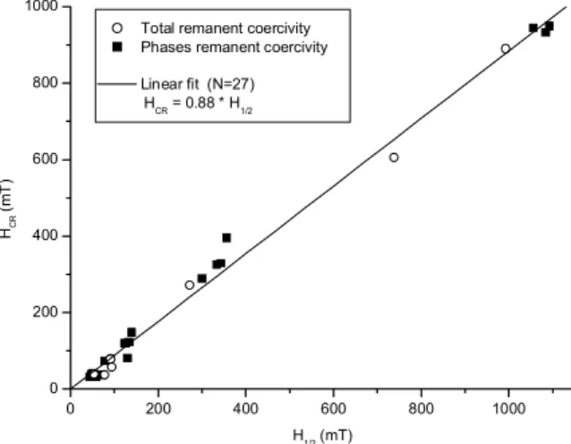
Although these parameters are obtained from two different connected measurements (back-field IRM and IRM acquisition curves) and they have differences, both are functionally related. A linkage between them (equation (2)) was tried to establish from the obtained results (N=27) summarised in Tables 1 and 2. From the study of linear regression fit, a very good correlation between both parameters was found, R=0.996 (Fig. 8). The following linear relationship was found,
HC R =0.88∗H1/2 (2)
and therefore, HCR/H1/2 =0.88±0.01for total and individual
Table 4. Statistics, F-tests and t-test, for two interpretations (fit1 and fit2) for each numerical method. Tabla 4.Pruebas estadísticas, prueba-F y prueba-t, para las dos interpretaciones (fit1 y fit2) para cada método numérico (CLG y UM).
Sample F-test t-test Test results
MgSth2 fit1 and fit2 (CLG) LAP 1,03 1,54 No difference
GAP 1,51 0,38 No difference
SAP 231,78 fit1 better
fit1 and fit2 (UM) LAP 1,50 0,21 No difference
GAP 1,09 0,03 No difference
SAP 1,23 0,16 No difference
HmSth3 fit1 and fit2 (CLG) LAP 4,07 fit1 better
GAP 1,42 0,09 No difference
SAP 29,35 fit1 better
fit1 and fit2 (UM) LAP 3,13 fit1 better
GAP 1,16 0,32 No difference
SAP 781,14 fit1 better
HmMgSth1 fit1 and fit2 (CLG) LAP 210,49 fit1 better
GAP 1,82 0,29 No difference
SAP 2,10 fit1 better
fit1 and fit2 (UM) LAP 4,12 fit1 better
GAP 1,10 0,36 No difference
SAP 1,03 0,00 No difference
HmMgSth2 fit1 and fit2 (CLG) LAP 4,61 fit1 better
GAP 1,01 0,09 No difference
SAP 2,13 fit2 better
fit1 and fit2 (UM) LAP 1,46 0,67 No difference
GAP 1,07 0,05 No difference
SAP 1,24 0,09 No difference
PE1a8 fit1 and fit2 (CLG) LAP 2,91 fit2 better
GAP 1,70 0,31 No difference
SAP 1,78 0,11 No difference
fit1 and fit2 (UM) LAP 14,67 fit1 better
GAP 1,83 0,45 No difference
SAP 1,73 0,89 No difference
PE1a12 fit1 and fit2 (CLG) LAP 9,00 fit2 better
GAP 1,12 0,20 No difference
SAP 1,95 fit1 better
fit1 and fit2 (UM) LAP 1,35 0,26 No difference
GAP 1,13 0,13 No difference
SAP 1,79 0,31 No difference
GoP2 fit1 and fit2 (CLG) LAP 4,69 fit1 better
GAP 1,33 0,24 No difference
SAP 1,57 0,16 No difference
fit1 and fit2 (UM) LAP 10,31 fit1 better
GAP 2,05 fit1 better
SAP 4,46 fit1 better
Goeth1b fit1 and fit2 (CLG) LAP 2,51 fit1 better
GAP 1,32 0,17 No difference
SAP 8,19 fit1 better
fit1 and fit2 (UM) LAP 3,67 fit2 better
GAP 6,02 fit1 better
SAP 6,59 fit1 better
5 and250µm (PSD and MD grains). On the other hand, Dunlop (1986) extended the grain size range of magnetite studying sub-micron magnetites, ranging between 0.04 and0.22µm (SD and
PSD grains). He obtained HCR/H1/2 ratios varying from 0.67 to 0.80. According to both studies, this ratio increases from MD to PSD to SD grains, and they give an entire magnetite interval that ranges from 0.55 to 0.80.
0 200 400 600 800 1000
0 200 400 600 800 1000
HC
R
(m
T
)
H1/2 (mT) Total remanent coercivity Phases remanent coercivity
Linear fit (N=27) HCR = 0.88 * H1/2
Figure 8– Remanent coercivity (HCR) vs remanent coercivity acquisition (H1/2) for Total and Phases data from all samples, synthetic and natural samples. Figura 8–Coercitividad remanente (HCR) versus coercitividad remanente de adquisici´on (H1/2) para datos de Fases y Totales de todas las muestras (sint´eticas y naturales).
The proposed relationship (equation 2) agrees very well with results obtained by Dankers (1981) and Dunlop (1986). It should be taken into account that the data used in our linear fit are ”pure”and mixed samples involving magnetites, maybe titano-magnetites, hematites and goethites. Therefore such relationship (equation 2) might have a more global character. HCR/H1/2 ra-tios from individual soft and hard phases show differences in-between, that are supported by the above mentioned interval of coercitivity values for magnetite, titanomagnetite and hematite. It is worth mentioning that Total HCR/H1/2ratios (as well as other ratios, e.g. S-ratio) of mixed samples are influenced by contribu-tion of soft/hard materials, i.e. HCR/H1/2is 0.82 for a magnetically harder sample (HmMgSth1), and on the other hand, 0.61 for a magnetically softer sample (HmMgSth2).
Remarks for the proposed method
From these results we can see that the research on the proposed method must go further in order to improve it. Variables to be ta-ken into account are related with AF demagnetisation; one of them is the selected peak AF value, which determines the AF filter be-cause the response of each mineral and their different grain size is different. Other variable is the AF decay rate for thetumbling
method(Dankers, 1978; Egli and Lowrie, 2002). If AF is not slo-wly reduced to zero, and the specimen is not quickly rotated, the remanence with coercivities lower than the peak AF might not be cancelled out randomly. Therefore some directions might not be suitably swept and consequently the intensity of remanent mag-netisation will be affected. The above mentioned inaccuracy for several non-significant contributions of Phases could be remo-ved if these variables are taken into account.
If the saturation of magnetically hard minerals is not reached, it might be difficult to calculate some parameters from its corres-ponding phase, especially H1/2 and SIRM because they can be underestimated. However, such problem can only arise for hard materials (especially goethite and hematite), so this difficulty can be solved using higher pulse magnetising fields and rearranging the growing field steps. On the other hand, discrimination itself can be successfully carried out even if the hard phase has not re-ached its saturation remanence.
From section 5.3, it is possible to conclude that there is satis-factory agreement between theexperimental methodand numeri-cal methods. The experimental method is more time-consuming than the other. However, this method provides anexperimental
and therefore, a morerealisticdiscrimination into individual pha-ses contributing to Total IRM curve.
Finally, we think that fruitful results can be obtained using al-ternatively the experimental and numerical methods. For instance, the experimental method might be applied to pilot samples and information about the expected number of individual contributing curves can be obtained. Then this extra information can be taken into account in order to model IRM curves for the rest of samples by using numerical methods.
Another interesting possibility is the joint use of both kind of methods, i.e. experimental method can be used to discriminate main phases and then numerical methods can be applied to each phase or residual curve in order to investigate it in a more detailed way.
CONCLUSIONS
mag-netic phases in natural samples that could not be observed by using other methods, at least without additional information.
A linear relationship between remanent coercivities, HCRand H1/2, was established for every phase. The calculated slope from equation 2 (or HCR/H1/2 = 0.88) involves data of soft/hard pha-ses and both of them, hence it is interpreted as a global result. It is worth mentioning that HCR/H1/2ratio for individual phases corresponds to characteristic values according to Dankers (1981) and Dunlop (1986).
The method was carried out using two peak AF values of 50 and 102.5 mT as a first try. Different or more convenient peak AF values could be selected, in order to discriminate minerals with another coercivity spectrum and also to improve separation between phases. In order to achieve improvements for the method, it will be necessary to research the effect of several AF demagneti-sation variables in an exhaustive way, such as peak AF, decay rate of AF, etc.
The discrimination obtained using ourexperimental method
agrees with results obtained from purely numerical methods. Although our experimental method is more time-consuming than others, it provides an experimental and realistic discrimination into individual phases contributing to the Total IRM measure-ments.
This method is also successfully applied to backfield IRM measurements, obtaining S-ratios and HCRparameters for each phase that cannot be determined by other methods. The reliability of S-ratio and HCRis supported by the results of mixing synthetic samples, since the results for each main phase agree with those obtained for unmixed synthetic samples.
ACKNOWLEDGEMENTS
The authors wish to thank the Universidad Nacional del Centro de la Provincia de Buenos Aires (UNCPBA) and CONICET for finan-cial support. Many thanks to C. Vasquez and J. C. Bidegain for the provided samples.
The authors are really indebted to the anonymous reviewer for his useful commentaries and suggestions.
REFERENCES
ARGYLE KS, DUNLOP DJ and XU S. 1994. Single-domain behaviour of multidomain magnetite grains. Abstract Eos (Trans. Am. Geophys. Un.), 75, Fall Meeting suppl., 196.
BAILEY ME and DUNLOP DJ. 1983. Alternating field characteristics of
pseudo-single domain (2-14µm) and multidomain magnetite. Earth
Pla-net. Sci. Lett., 63: 335–352.
BLOEMENDAL J, KING JK, HALL FR and DOH SJ. 1992. Rock magne-tism of Late Neogene and Pleistocene deep-sea sediments: Relationship to sediment source, diagenetic processes and sediment lithology. J. Ge-ophys. Res., 97: 4361–4375.
CHAPARRO MAE, BIDEGAIN JC, SINITO AM, GOGORZA CS and JU-RADO S. 2002a. Preliminary Results of Magnetic Measurements on Stream-Sediments from Buenos Aires province, Argentina. Studia Geo-physica et Geodaectia, 47(1): 121–145.
CHAPARRO MAE, BIDEGAIN JC, SINITO AM, GOGORZA CS and JU-RADO S. 2002b. Comparison of Magnetic Studies of Soils and Stream-Sediments from Buenos Aires Province (Argentina) Applied to Pollution Analysis. Extended abstract for the International Symposium on Fun-damental Rock Magnetism and Environmental Applications. Erice, Italy, 25–27.
CHAPARRO MAE, SINITO AM and BIDEGAIN JC. 2003. Estudios
Magn´eticos sobre Goethita (α-FeOOH) Natural de Tharsis (Huelva,
Espa˜na). Boletin Geol´ogico y Minero Espa˜nol, (submitted).
DANKERS PHM. 1978. Magnetic properties of dispersed natural iron-oxides of known grain-size, thesis, State University of Utrecht, 142 pp.
DANKERS PHM. 1981. Relationship between median destructive field and remanent coercive forces for dispersed natural magnetite, titanomag-netite and hematite. Geophys. J. R. Astr. Soc., 64: 447–461.
DE BOER CB and DEKKERS MJ. 1998. Thermomagnetic behaviour of he-matite and goethite as a function of grain size in various non-saturating magnetic fields. Geophys. J. Int., 133: 541–552.
DUNLOP DJ. 1986. Coercive forces and coercivity spectra of submicron magnetites. Earth and Planet. Sci. Lett., 78: 288–295.
DUNLOP DJ and ¨OZDEMIR ¨O. 1997. Rock magnetism. Fundamentals and frontiers. Cambridge University Press. 573 pp.
EGLI R and LOWRIE W. 2002. Anhysteric remanent magnetization of fine magnetic particles. J. Geophys. Res., 107(B10): 2209, doi: 10.1029/2001JB000671.
FRANCE DE and OLDFIELD F. 2000. Identifying goethite and hematite from rock magnetic measurements of soils and sediments. J. Geophys. Res., 105 (B2): 2781–2795.
HESLOP D, DEKKERS MJ, KRUIVER PP and VAN OORSCHOT IHM. 2002. Analysis of isothermal remanent magnetisation acquisition curves using the expectation-maximisation algorithm. Geophys. J. Int., 148: 58–64.
KRUIVER PP, DEKKERS MJ and HESLOP D. 2001a. Quantification of magnetic coercivity components by the analysis of acquisition curves of isothermal remanent magnetisation. Earth and Planet. Sci. Lett., 189: 269–276.
an investigation of the S ratio. Geochem. Geophys. and Geosys. Paper number 2001GC000181.
MAHER BA, THOMPSON R and HOUNSLOW MW. 1999. Introduction. In: Quaternary Climate, Environments and Magnetism (Maher B.A. and Thompson R., eds.), 1-48 pp. Cambridge University Press, Cambridge.
PETERS C and THOMPSON R. 1998. Magnetic identification of selected natural iron oxides and sulphides. J. Magn. Magn. Mater., 183: 365– 374.
PETERS C, DEKKERS MJ and LANGEREIS CG. 2002. Validation of mine-ral magnetic methods. Extended abstract for the International Symposium on Fundamental Rock Magnetism and Environmental Applications. Erice, Italy, 129–130.
ROBERTSON DJ and FRANCE DE. 1994. Discrimination of remanence-carrying minerals in mixtures using isothermal remanent magnetization
acquisition curves. Phys. Earth Planet. Int., 82: 223–234.
STOCKHAUSEN H. 1998. Some new aspects for the modelling of isother-mal remanent magnetization acquisition curves by cumulative log Gaus-sian functions. Geophys. Res. Lett., 25 (12): 2217–2220.
THOMPSON R and OLDFIELD F. 1986. Environmental magnetism. Allen & Unwin (Publishers) Ltd., 225 pp.
WOHLFARTH EP. 1958. Relations between different modes of acquisition of the remanent magnetization of ferromagnetic particles. J. Appl. Phys., 29: 595–596.
WORM HU. 1999. Time-dependent IRM: A new technique for magnetic granulometry. Geophysical Res. Ltrs. 1999GL008360, 26 (16): 2,557.
XU S and DUNLOP DJ. 1995. Towards a better understanding of the Lowrie-Fuller test. J. Geophys. Res., 100: 22,533–22,542.
NOTES ABOUT THE AUTHORS
Marcos Adri´an Eduardo Chaparrowas born on April 17th1972 in San Cayetano (Argentina); he began his research in physics in 1996 before he obtained his M.Sc. degree in Physics in Nov 1999. After on, he began his PhD studies in Physics and has been actively involved in Geomagnetism research, namely magnetic signature of anthropogenic pollution in river sediments and soils. Current Position: Teaching Assistance, Facultad de Ciencias Exactas, UNCPBA. Postgraduate Fellow of National Council of Scientific and Technical Research of Argentina (CONICET). Research Interest: Environmental magnetism, Magnetic properties of materials, Experimental Methods of Rock-magnetism. Paleomagnetism on lake sediments.
Web site: http://www.exa.unicen.edu.ar/ifas/paleomag.html