www.scielo.br/rbg
A QUICK REVIEW OF 2D TOPOGRAPHIC TRAVELTIMES
German Garabito
1, Pedro A. Chira-Oliva
2, Martin Tygel
3and L´ucio T. Santos
4Recebido em 6 janeiro, 2005 / Aceito em 10 marc¸o, 2005 Received on January 6, 2005 / Accepted on March 10, 2005
ABSTRACT.The Common-Reflection-Surface (CRS) stacking method was originally introduced as a data-driven method to simulate zero-offset sections from 2-D reflection pre-stack data acquired along a straight line. This approach is based on a second-order hiperbolic traveltime approximation parameterized with three kinematic wavefield attributes. In land data, topographic effects play an important role in seismic data processing and imaging. Thus, this feature has been recently considered by the CRS method. In this work we review the CRS traveltime approximations that consider the smooth and rugged topography. In addition, we also review the Multifocusing traveltime for a rugged topography. By means of a simple synthetic example, we finally provide first comparisons between the various traveltime expressions.
Keywords: Traveltime, CRS, Multifocus, Topography.
RESUMO.O m´etodo de empilhamento Superf´ıcie de Reflex˜ao Comum (SRC) foi originalmente introduzido como um m´etododata-driven para simular sec¸˜oes afastamento-nulo a partir de dados s´ısmicos de reflex˜ao pr´e-empilhados 2-D adquiridos ao longo de uma linha de aquisic¸˜ao reta. Este m´etodo est´a baseado em uma aproximac¸˜ao de tempos de trˆansito hiperb´olica de segunda ordem parametrizada com trˆes atributos cinem´aticos do campo de onda. Em dados terrestres, os efeitos topogr´aficos desempenham um papel importante no processamento e imageamento de dados s´ısmicos. Assim, esta caracter´ıstica tem sido considerada recentemente pelo m´etodo SRC. Neste trabalho apresentamos uma revis˜ao das aproximac¸˜oes de tempos de trˆansito SRC que consideram topografia suave e rugosa. Adicionalmente, n´os revemos tamb´em a aproximac¸˜ao de tempos de trˆansito Multifoco para o caso da topografia rugosa. Por meio de um exemplo sint´etico simples, n´os fornecemos finalmente as primeiras comparac¸˜oes entre as diferentes express˜oes de tempos de trˆansito.
Palavras-chave: Tempos de trˆansito SRC, Multifoco, Topografia.
1 Universidade Federal do Par´a, Departamento de Geof´ısica, Rua Augusto Corrˆeia, 01, Campus Universit´ario do Guam´a, Caixa Postal 1611 – CEP: 66.017-970; Tel.: (91)211-1473 / Fax: (91)211-1671 – E-mail: [email protected]
2 Universidade Federal do Par´a, Departamento de Geof´ısica, Rua Augusto Corrˆeia 1, Campus Universit´ario do Guam´a, Caixa Postal 1611 – CEP 66017-970; Tel: (091) 3183-1473; Fax: (091) 3183-1671 – E-mail: [email protected]
3 UNICAMP – IMECC, Prac¸a Sergio Buarque de Holanda, 651, Cidade Universit´aria, Bar˜ao Geraldo, Caixa Postal 6065 – 13083-859 Campinas, S˜ao Paulo, Brasil – E-mail: [email protected]
INTRODUCTION
The Common-Reflection-Surface (CRS) and the Multifocus (MF) methods are designed to produce clear stacked sections and useful time-domain attributes by means of coherence analysis methods directly applied to multicoverage reflection data. In this way, both methods, that have a similar purpose and approach as the well-established common-midpoint (CMP) method, represent powerful extensions of the latter. As opposed to the CMP method that is applied to CMP gathers and extracts a single parameter (the normal-moveout (NMO) velocity) on manually picked events, the CRS and MF methods (a) make full use of the available multico-verage data by applying the stacking procedure on supergathers that are free from the CMP restriction; (b) extract more parameters (three in the 2D situation) at each time sample of the stacked sec-tion to be constructed and (c) the procedure is applied to all time samples without the need of event selection. The CRS and MF methods fall into the category of the so-called macro-model in-dependent or data-driven time-domain methods (see, e.g., Hubral (1999) for a general account and discussion).
A distinctive feature of the CRS and MF methods is the use of specific multiparameter traveltime moveouts. The parameters of these moveout expressions are directly inverted from the data by means of coherence analysis (semblance) procedures. With the help of the inverted parameters, the obtained moveouts are employed to stack the data. Note that this is exactly what the con-ventional velocity analysis method does under the restriction of the one-parameter NMO traveltimes applied to CMP gathers.
Originally, both the CRS and the MF have been derived un-der the following assumptions: (a) 2D propagation; (b) locally-constant and supposedly known near-surface velocity and (c) no topographic effects along the seismic line. The latter condition means that the data have been acquired on a horizontal seismic line or preprocessed for statics and residual statics to a horizontal datum before the application of the CRS or MF method.
Under these considerations, the CRS and MF moveouts are expressed as functions of three parameters, namely the emergence angle,β0, of the zero-offset (ZO) ray with respect to the (planar)
surface normal, and two wavefront curvatures,KN I PandKN,
of the so-called NIP- and N-waves that relate to the ZO ray at its emergence point. We recall that the abbreviation NIP stands for normal-incident-point, namely the point where the ZO ray hits the reflector and that the NIP-wave is a fictitious wave that starts as a point source at NIP and progresses upwards to the measure-ment surface with half the medium velocity. In the same way, the
a fictitious wave that starts as a wavefront with the shape of the reflector at NIP and progresses upwards with half of the medium velocity. For detailed description and discussion of the NIP- and N-waves, the reader is referred to Hubral (1983).
It is to be observed that the CRS and MF methods can also be normally applied in the case the above requirements are not met. In that case, the three-parameter CRS and MF represent simply stacking parameters that provide a best fit to the reflection events, but cannot be directly attached to the above-mentioned seismic propagation attributes (angles and curvatures). For example, the classical CRS and MF expressions consider the condition of a locally constant near-surface velocity. This means that that the near-surface velocity is considered constantin the vicinity of each central point but can vary as we change from each central point to another. To be consistent with the second-order formulation, the traveltime expression has to consider, not only the velocity, but also its gradient at each central point. As a consequence, wrong near-surface velocities will give rise to wrong emerging angles, even though correct ray parameters can be extracted. In the same way, topographic effects, if not correctly taken into account, will contaminate the CRS attributes affecting their interpretation.
For a planar or smoothly curved measurement surface, the 2D CRS (hyperbolic) traveltime that takes full consideration of the velocity gradient at the central point is presented in Chira et al. (2001). In the MF traveltime expressions, velocity gradients at the central points are not considered. To our knowledge, exam-ples of the influence of the velocity gradients have not yet been provided in the literature.
In this paper, the usual assumption of a locally-constant near-surface velocity will be also adopted, our attention being concen-trated on the incorporation of topography into the traveltime ex-pressions.
2D CRS AND MF TRAVELTIMES FOR A PLANAR MEASUREMENT SURFACE
X0=(x0,0). We denotem=xm−x0, byT0the (two-way)
reflection time along the ZO (central) ray and byv0the velocity at
the central point. As explained above, we assume that the velo-city remains constant for all source-receiver locations where the
traveltime is to be computed. Finally,β0,KN I PandKNdenote
the emergence angle and the curvatures of the NIP and N waves that refer to the ZO ray as observed atX0. Under these
conside-rations, the CRS traveltime reads (see, e.g., J¨ager et al. (2001))
TC R S2 (m,h)=
T0+
2 sinβ0
v0 m
2
+2T0 cos 2β
0
v0
KN m2+KN I P h2
. (1)
For the same situation of a planar measurement surface, the corresponding 2D MF traveltime is given by (see, e.g., Gelchinsky et al. (1999) with a different notation)
TM F(m,h)=T0 +
1
v0 KS
[KS(m−h)+sinβ0]2+cos2β0−1
+ 1
v0 KG
[KG (m+h)+sinβ0]2+cos2β0−1
, (2)
where
KS=
KN−σ KN I P
1−σ , KG =
KN+σ KN I P
1+σ , (3)
and
σ = h
m+(m2−h2)K
N I P sinβ0
. (4)
CRS APPROXIMATION FOR SMOOTH TOPOGRAPHY
The CRS traveltime expression (1) admits a natural extension to the case of a smoothly curved measurement surface. More speci-fically, let us assume that, at the central point and with respect to a horizontal datum, the seismic line has curvature,K0and dipα0.
See Figure 1(a). Moreover, letγ0denote the emergence angle of
the ZO central ray with respect to the normal to the curved seismic line at the central point. As shown in Chira (2003) (with a different notation), the CRS traveltime for a source-receiver pair located by (m,h)is given by
TC R S2 (m,h)=
T0+
2 sinγ0
v0cosα0 m
2
+2T0 cosγ0
v0cos2α0
[KN cosγ0−K0] m2
+2T0 cosγ0
v0cos2α0
[KN I P cosγ0−K0]h2.
(5)
We ready verify that, in the case of a horizontal seismic line, we haveK0=α0=0andγ0=β0, so that equation (5) reduces
to its previous counterpart equation (1), as expected.
As reported in Chira (2003), the traveltime moveout (5) were tested for a synthetic model of smooth topography with good re-sults. The formulation breaks down, however, as the topography
becomes more pronounced.
CRS AND MF APPROXIMATIONS FOR RUGGED TOPO-GRAPHY
We now consider the extension of the CRS traveltime to the case of arbitrary (rugged) topography. Following Zhang et al. (2002), we find useful to considervectormidpoint,m, and half-offset,h, co-ordinates with respect to the Cartesian system of horizontal datum and downward vertical. See Figure 1(b). More specifically, we set m=(mx,mz)andh=(hx,hz)which locate the
correspon-ding source and receiver pair asS =m−handG=m+h, respectively. As shown in Zhang et al. (2002), we have
TC R S2 (m, h)=
T0− 2
v0
(mx sinβ0+mz cosβ0)
2
+2T0 KN
v0
(mx cosβ0−mz sinβ0)2 (6)
+2T0 KN I P
v0
(hx cosβ0−hz sinβ0)2 .
z
x x
0
Measurement Surface
G S
x
m
2h
Central Ray γ0
α0
(a) β0
z
x x0
Central Ray β0
S
G
m
h
(b)
Figure 1– Cartesian system of coordinates for: (a) Smooth topography; (b) Rugged topography.
TM F(m, h)=t0 + 1
v0KS
[KS(mx−hx)+sinβ0]2+ [KS(mz−hz)+cosβ0]2−1
+ 1
v0KG
[KG(mx+hx)+sinβ0]2+ [KG (mz+hz)+cosβ0]2−1
, (7)
where
KS =
KN−σ KN I P
1−σ , KG =
KN+σ KN I P
1+σ , (8)
σ = hx −hz tanβ0
mx−mz tanβ0+Q KN I P sinβ0
, (9)
and
Q=(m2x−h2x−m2z+h2z)+(mx mz−hx hz)cos 2β0. (10)
NUMERICAL EXPERIMENTS
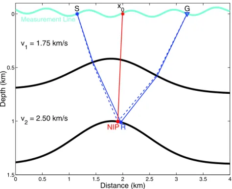
In order to check the accuracy of the traveltime formulas dis-cussed in this work, we consider the simple 2D model de-picted in Figure 2. It consists of two homogeneous acous-tic layers, with velocities 1.75 km/s and 2.5 km/s, respecti-vely, separated by a curved interface. The measurement line has a rugged (nonsmooth) topography. We have used the ray tracing package SEIS88 ( ˇCerven´y & Psˇensik, 1988) to model the reflection traveltimes for the reflecting interface. We have simulated a multiple coverage around the central point with
x0=2 km.
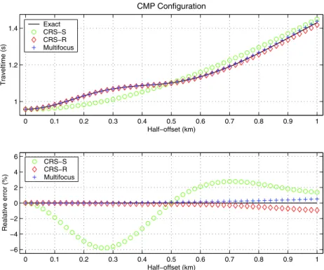
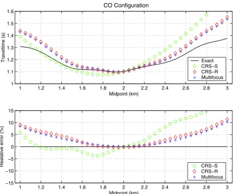
Figures 3–5 show the modelled reflection traveltimes for three
(CO) and Common-Midpoint (CMP), and the respective approxi-mation formulas, CRS smooth [CRS-S], equation (5), CRS rugged [CRS-R], equation (6), and Multifocus, equation (7). Also depic-ted are the relative errors for the three approximations.
As readily observed, the CRS-S formula gives poor appro-ximations, whereas CRS-R and Multifocus present good results with relative errors of the same order.
0 0.5 1 1.5 2 2.5 3 3.5 4 0
0.5
1
1.5
Distance (km)
Depth (km)
Measurement Line
v
1 = 1.75 km/s
v
2 = 2.50 km/s
x 0
S G
NIPR
Figure 2– 2D acoustic model for the numerical experiments. The ZO ray is ploted in red, the reflection ray in blue and the diffraction ray in dashed blue. Also indicated are the normal-incidend-point (NIP) and the reflection point (R).
2 2.2 2.4 2.6 2.8 3 3.2 3.4 3.6 3.8 4
1 1.2 1.4 1.6 1.8 2
Receiver x−coord. (km)
Traveltime (s)
CS Configuration
Exact CRS−S CRS−R Multifocus
2 2.2 2.4 2.6 2.8 3 3.2 3.4 3.6 3.8 4
−20 −10 0 10 20
Realative error (%)
Receiver x−coord. (km) CRS−S
CRS−R Multifocus
1 1.2 1.4 1.6 1.8 2 2.2 2.4 2.6 2.8 3 1
1.1 1.2 1.3 1.4 1.5 1.6
Traveltime (s)
Midpoint (km)
CO Configuration
Exact CRS−S CRS−R Multifocus
1 1.2 1.4 1.6 1.8 2 2.2 2.4 2.6 2.8 3
−15 −10 −5 0 5 10 15
Realative error (%)
Midpoint (km) CRS−S
CRS−R Multifocus
Figure 4– Reflection traveltime approximations for a CO configuration withh=0.5km.
0 0.1 0.2 0.3 0.4 0.5 0.6 0.7 0.8 0.9 1
1 1.2 1.4
Half−offset (km)
Traveltime (s)
CMP Configuration
Exact CRS−S CRS−R Multifocus
0 0.1 0.2 0.3 0.4 0.5 0.6 0.7 0.8 0.9 1
−6 −4 −2 0 2 4 6
Realative error (%)
Half−offset (km) CRS−S
CRS−R Multifocus
2 2.2 2.4 2.6 2.8 3 3.2 3.4 3.6 3.8 4 1
1.2 1.4 1.6 1.8 2
Receiver x−coord. (km)
Traveltime (s)
CS Configuration
Exact CRS−S CRS−R Multifocus
2 2.2 2.4 2.6 2.8 3 3.2 3.4 3.6 3.8 4
−20 −10 0 10 20
Realative error (%)
Receiver x−coord. (km)
CRS−S CRS−R Multifocus
Figure 6– Diffraction traveltime approximations for a CS configuration withxS=2.0km.
1 1.2 1.4 1.6 1.8 2 2.2 2.4 2.6 2.8 3
1 1.1 1.2 1.3 1.4 1.5 1.6
Traveltime (s)
Midpoint (km)
CO Configuration
Exact CRS−S CRS−R Multifocus
1 1.2 1.4 1.6 1.8 2 2.2 2.4 2.6 2.8 3
−15 −10 −5 0 5 10 15
Realative error (%)
Midpoint (km)
CRS−S CRS−R Multifocus
Garabito et al. (2003) in the case of Marmousi data with good re-sults. Figures 6 and 7 depict the results obtained in the present experiment. Observe that the CMP configuration is not shown since the traveltime expressions are the same as in the previous case.
As expected, the relative errors were now increased. Once again, the S formula has the worst behaviour whereas CRS-R and Multifocus formulas behave similarly. We verify that, for small aperture the relative errors remain very reasunable, so that the CRS-R and Multifocus formulas for diffraction traveltimes are able to well approximate the exact (modelled) reflection travelti-mes. As a conclusion, a two-parameter search in the CRS method usingKN I P = KN in the formulas, have the potential of
pro-ducing good initial approximations for the CRS attributes.
CONCLUSIONS
We quickly revisited the Common-Reflection-Surface (CRS) and Multifocus traveltime moveouts in the case of a topographic me-asurement surface. By means of a simple synthetic example, we provided first comparisons on their accuracy and validity. Our re-sults show that the approximation formulas for rugged topography yield good results, not only to approximate the exact (modelled) reflection traveltimes, but also as a two-parameter formula in the search for initial approximations for the CRS attributes.
ACKNOWLEDGMENTS
This work has been partially supported by theNational Coun-cil of Scientific and Technological Research (CNPq), and Rese-arch Foundation of the State of S˜ao Paulo (FAPESP), Brazil. We
also thank the sponsors of theWave Inversion Technology (WIT) Consortium.
REFERENCES
ˇCERVEN´Y V & PSˇENSIK I. 1988. Ray tracing program package, Charles University, Czechoslovakia.
CHIRA P, TYGEL M, ZHANG Y & HUBRAL P. 2001. Analytic CRS Stack formula for a 2D curved measurement surface and finite-offset reflections, Journal of Seismic Exploration, 5: 245–262.
CHIRA P. 2003. Empilhamento pelo m´etodo Superf´ıcie de Reflex˜ao Co-mum 2-D com Topografia e Introduc¸˜ao ao caso 3-D, Federal University of Para, Brazil.
GARABITO G, CRUZ JCR, HUBRAL P & TYGEL M. 2003. 2-D Common-Reflection-Surface (CRS) stack based on simulated annealing and quasi-Newton: Application to Marmousi data set, 7th WIT Report.
GELCHINSKY B, BERKOVITCH A & KEYDAR S. 1999. Multifocusing ho-meomorphic imaging, Part I: Basic concepts and formulas, Journal of Applied Geophysics, 42: 229–242.
GUREVICH B, KEYDAR S & LANDA E. 2002. Multifocusing imaging over an irregular topography, Geophysics, 67: 639–643.
HUBRAL P. 1983. Computing true amplitude reflections in a laterally inhomogeneous Earth, Geophysics, 48: 1051–1062.
HUBRAL P. 1999. Macro-model independent seismic reflection imaging, Journal of Applied Geophysics, 42: 137–148.
J¨AGER R, MANN J, H ¨OCHT G & HUBRAL P. 2001. Common-reflection-surface stack: Image and attributes, Geophysics, 66: 97–109.
ZHANG Y, H ¨OCHT G & HUBRAL P. 2002. Extended Abstracts, “Poster 166”, 2D and 3D ZO CRS stack for a complex top-surface topography, 64th Annual Internat. Mtg., Eur. Assoc. Expl. Geophys.
NOTES ABOUT THE AUTHORS
German Garabitoreceived his BSc (1986) in Geology from University Tom´as Frias (UTF), Bolivia, his MSc in 1997 and PhD in 2001 both in Geophysics from the Federal University of Par´a (UFPA), Brazil. Since 2002 he has been full professor at the geophysical department of UFPA. His research interests are data-driven seismic imaging methods such as the Common-Refection-Surface (CRS) method and velocity model inversion.
Pedro Chira-Olivareceived his diploma in Geological Engineering (UNI-Peru/1996). He also received his MSc in 1997 and PhD in 2003, both in Geophysics, from Federal University of Par´a (UFPA/Brazil). He took part of the project of scientific research i“3D Zero-Offset Common-Reflection-Surface (CRS) stacking” (2000-2002), sponsored by Oil Company ENI (AGIP Division - Italy) and the University of Karlsruhe (Germany). Since 2003 he is researcher of the UFPA, responsible for the scientific project “Generalization of the Common-Reflection-Surface (CRS) stacking applied to real data in the Amazon region”, financed by the PROSET/CT-PETRO/CNPq. He is an associate member of the Society of Exploration Geophysicists (SEG), Brazilian Geophysical Society and also is member of the Wave Inversion Technology (WIT) Corsortium (Germany).
1992 as a full professor in Applied Mathematics. Professor Tygel has been an Alexander von Humboldt fellow from 1985 to 1987. In that period, he conducted research at the German Geological Survey (BGR) in Hannover. From 1995 to 1999, he was the president of the Brazilian Society of Applied Mathematics (SBMAC). In 2002, he received EAGE’s Conrad Schlumberger Award and also UNICAMP’s Zeferino Vaz Award for academic recognition in 1995 and 2004. Prof. Tygel is the founder in 2001 of the Laboratory of Geophysical Computing at UNICAMP. The Laboratory is a member of the Wave Inversion Technology (WIT) Consortium, with headquarters in Karlsruhe. Prof. Tygel’s research interests are in seismic processing, imaging and inversion. Emphasis is aimed on methods and algorithms that have a sound wave-theoretical basis and also find significant practical application.