Image analysis of Saccharomyces cerevisiae cells : development of a plugin for IMAGEJ

(1)

Vítor Damião Baixinho da Silva

Image analysis of

Saccharomyces cerevisiae

cells: Development of

a plugin for ImageJ

Dissertation of Master in Bioinformatics

Work supervised by:

Eugénio Manuel de Faria Campos Ferreira

and

Daniela Patrícia Bernardino Mesquita

(2)

(3)

Acknowledgements/Agradecimentos

Todo este trabalho não teria sido possível de realizar sem as ações multifacetadas dos seguintes intervenientes, aos quais tenho o maior prazer de mencionar e prestar o meu agradecer:

O Professor Doutor Eugénio Manuel de Faria Campos Ferreira que se disponibilizou de imediato em orientar-me neste projeto, motivando-me com total empenho, a ele agradeço a oportunidade concedida em realizar este estudo, bem como todas as sugestões críticas e reuniões.

Muito devo à dedicação e empenho da Doutora Daniela Patrícia Bernardino Mesquita na supervisão do meu projeto, ficando-lhe imensamente agradecido pela sua motivação e incentivo no trabalho desenvolvido, no qual resulta esta dissertação.

Enalteço o Doutor Marek Mösche, pela oportunidade concedida em participar neste projecto. Um especial agradecimento deixo à colega Susanne Polap, por todas as imagens de levedura e ajudas fornecidas para o desenvolvimento do estudo, uma vez que a sua inexistência tornaria muito difícil a realização deste trabalho.

Para finalizar, e não menos importante, gostaria de agradecer a todos os elementos da minha família por todo o apoio fornecido, caso contrário tudo isto não seria tão facilmente conseguido.

Acima de tudo, gostaria de mencionar a Helena Ferreira, uma das principais razões para finalizar este mestrado, ao qual lhe agradeço todo o apoio e paciência para comigo, me incentivando e motivando nos momentos mais difíceis.

Isto tudo foi possível e realizado com o apoio financeiro concebido pela empresa Uniferm – Bakery Ingredients.

(4)

(5)

Abstract

The yeast Saccharomyces cerevisiae is one of the microorganisms with increased use at industrial, academic and scientific level. The easy growth in any culture medium, as well as the complete sequencing of its genome, are two of the main interesting factors, making this microorganism one of the most important worldwide.

The morphological analysis of yeast using optical microscopy is a research area of great interest. Over the last decades, significant advances have been made in digital image processing as well in the analysis of microscopic images of cells. In this context, the development of specific software such as ImageJ is of particular interest since it is free access and open source.

The main goal of this work was to develop a computer program, in the form of an extension module (plugin), in order to add certain features to ImageJ software. For this purpose, programming and processing methods were applied for a more reliable evaluation of cell and finally implemented as an ImageJ plugin. The plugin code was carried out using the Java programming language, since certain required functions were not present in the main program source code. Results presented as .xls file included the identification of cells, as well as counting and cataloguing after images processing and analysis. The features developed in this work allowed the user to process and analyse different microscopic images of S. cerevisiae cells. Finally, the plugin code was tested using multiple images of S. cerevisiae. The final version has shown high efficiency in S. cerevisiae culture images with different exposure times. Nevertheless, the plugin code was able to detect almost all cells in the images and classify them as large, normal, small and bud.

(6)

(7)

Resumo

A levedura Saccharomyces cerevisiae é um dos microrganismos com maior utilização a nível industrial, académico e científico. A facilidade de crescimento em qualquer meio de cultura, assim como a completa sequenciação do seu genoma, são dois dos principais fatores que tornam este microrganismo dos mais importantes no mundo.

A análise morfológica de leveduras é uma das áreas. Nas últimas décadas, foram feitos avanços significativos no processamento de imagens digitais, bem como na análise de imagens microscópicas de células. Neste contexto, o desenvolvimento de software específico, tal como o ImageJ é de particular importância, uma vez que é de acesso livre e possui implementação livre e aberta (open source).

Este trabalho teve como principal objectivo o desenvolvimento de um programa de computador na forma de módulo de extensão (plugin) com a finalidade de adicionar determinadas funcionalidades ao software ImageJ. Para permitir ao utilizador do ImageJ uma avaliação fidedigna de imagens de células obtidas por microscopia, foram aplicados diversos métodos de processamento. O código do plugin foi desenvolvido utilizando a linguagem de programação Java, uma vez que certas funções exigidas não estavam presentes no código fonte do programa. Os resultados apresentados como tipo de arquivo .xls incluíram a identificação de células, bem como a contagem e catalogação após o processamento e análise de imagens. As funcionalidades desenvolvidas durante a execução deste trabalho permitem ao utilizador processar e analisar diferentes imagens de células de S. cerevisiae obtidas por microscopia. O código do plugin foi testado utilizando várias imagens de S. cerevisiae. A versão final revelou uma elevada eficiência na caracterização de imagens de culturas de S. cerevisiae com diferentes tempos de exposição. Foi ainda possível detetar quase todas as células presentes nas imagens e classificá-las como grandes, normais, pequenas e germinadas.

(8)

(9)

ACKNOWLEDGEMENTS/AGRADECIMENTOS ... III ABSTRACT ... V RESUMO ... VII CONTENTS ... IX LIST OF FIGURES ... XIII LIST OF TABLES ... XXV 1. INTRODUCTION ... 1 1.1. Motivation ... 1 1.2. Objectives ... 1 1.3. Dissertation structure ... 2 2. CONTEXT... 5 2.1. Saccharomyces cerevisiae ... 5 2.1.1. Cell cycle ... 6 2.1.2. Morphology ... 7

2.2. Image processing and analysis ... 9

2.2.1. Image sensing and acquisition ... 11

2.2.2. Image processing techniques ... 13

2.2.3. Image analysis techniques ... 17

2.2.4. Image analysis of S. cerevisiae cells ... 19

3. IMAGEJ ... 23

(10)

3.1.1. Image menu ... 25

3.1.2. Process menu... 27

3.2. Object counting with ImageJ ... 30

3.3. Writing ImageJ plugins ... 32

3.3.1. Compiling and running plugins ... 33

3.3.2. ImageJ API ... 33

3.3.3. Types of Plugins ... 40

3.3.4. Coding new plugins ... 43

4. METHODOLOGY AND ALGORITHMS ... 47

4.1. ScerevisiCounter´s Main Pipeline ... 47

4.1.1. Opening images ... 47

4.1.2. Methodologies configuration ... 48

4.1.3. Type of results ... 50

4.2. Methodology optimization ... 54

4.2.1. Processes ... 56

4.2.2. Image Process Optimization ... 59

4.2.3. Refining methodologies ... 62

4.3. Debugging ... 64

5. RESULTS AND DISCUSSION ... 67

5.1. Methodology optimization results ... 67

5.1.1. Group 1 experiments – Subtract Background study ... 68

5.1.2. Group 2 experiments – Unsharp mask study ... 77

5.1.3. Other images Group 2 experiments ... 84

5.2. Final Version ... 91

5.3. Boundaries determination ... 93

5.4. Manual and automatic counting ... 97

6. CONCLUSIONS AND FURTHER WORK ... 99

(11)

APPENDIX A – GROUP 1 RESULTS ... 105

APPENDIX B – GROUP 2 RESULTS 1 ... 115

APPENDIX C – GROUP 2 RESULTS 2... 123

APPENDIX D – GROUP 2 RESULTS 3 ... 131

APPENDIX E – GROUP 2 RESULTS 4... 139

APPENDIX F – GROUP 2 RESULTS 5 ... 147

APPENDIX G – GROUP 2 RESULTS 6 ... 155

APPENDIX H – GROUP 2 TABLE RESULTS ... 163

APPENDIX I – SACHAROMYCES CEREVISIAE PICTURES ... 177

(12)

(13)

List of figures

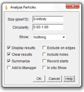
Figure 2.1. Schematic diagram for cell morphological changes used in cell cycle description (S phase: plaque duplication; G2 phase: nuclear migration; M phase: nuclear division; G1 phase: bud detachment) [10]. ... 7 Figure 2.2. Cell shape measurements of Saccharomyces cerevisiae cells (adapted) [16], [18]. .. 9 Figure 2.3. Mathematical notation for a digital image (adapted) [21]. ... 10 Figure 2.5. Plot of the first line (0 ≤ x ≤ 406 and y = 0) of a cell colony picture. The values, discretized to have a range corresponding to 8-bit images, demonstrate a good approximation of what would be the function curve for the values with continuous amplitude. ... 13 Figure 2.4. Cell colony image (available at http://imagej.nih.gov/ij/images). ... 13 Figure 2.6. Image of a cell colony (left picture) and their negative transformation (right picture) (available at http://imagej.nih.gov/ij/images). The transformation was possible using the Image Inverter plugin from software ImageJ... 14 Figure 2.7. Binarization of the cell colony image without filtering and after filtering. Figure 2.7a is the original cell colony image. Figure 2.7b is the result of thresholding the image of Figure 2.7a at pixel value 171. The image of Figure 2.7c is the result of applying a 5x5 median filter to the image of Figure 2.7a. The image of Figure 2.7d is the result of thresholding the image of Figure 2.7c at pixel value 171. All filter and threshold operations were performed with the support of the software ImageJ (available at [1]). ... 16 Figure 3.1. The ImageJ main window (version 1.48k). ... 25 Figure 3.2. Background subtraction of the cell colony image. Figure 3.2a is the original cell colony image (available at http://imagej.nih.gov/ij/images). Figure 3.2b results from the background subtraction of Figure 3.2a, with a rolling ball with 50 pixels of radius. The profile of Figure 3.2c is the plot of the yellow segment in the image of Figure 3.2a. The profile of Figure 3.2d is the plot of the yellow segment in the image of Figure 3.2b. ... 29 Figure 3.3. Analyze Particles window for particle counting operation of a thresholded image or 8-bit binary image. ... 31 Figure 3.4. ImageJ class diagram. ... 34 Figure 4.1. Particle analysis of a microscopic picture of yeast cells. Figure 4.1a is an 8-bit picture of two yeast cells. The image in Figure 4.1b is the result from auto thresholding the image from

(14)

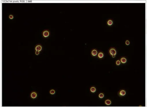
Figure 4.1a.Figures 4.1c and 4.1d are the mask and outlines resulting from the particle analysis of the image from Figure 4.1b, respectively. ... 49 Figure 4.2. Microscopic image (200 ms of exposure time) of a group of S. cerevisiae cells. One of the cells is cut by the edge of the picture and one of the visible spheres is not counted as a cell due to the reduced size, both of which are not accounted by ScerevisiCounter plugin. ... 52 Figure 4.3. Microscopic image (200 ms of exposure time) of a group of S. cerevisiae cells. Two cells may be considered as buds due to the protuberance in its edge. ... 53 Figure 4.4. Image 1 of 2 from the stack returned after processing the images of Figures 4.2 and 4.3 with the ScerevisiCounter plugin. This image refers to the image in Figure 4.2. It can be verified that all the cells were enumerated and properly marked by a blue outline, except the cell cropped by the edge of the image and near the lower left corner of the image. Small particles or debris were not processed. ... 54 Figure 4.5. Image 2 of 2 from the stack returned after processing the images of Figures 4.2 and 4.3 with the ScerevisiCounter plugin. This image refers to the image of Figure 4.3. All cells were properly enumerated and marked by a blue outline. The numbering was done synchronously with the numbering of the picture 1 of 2 of the final stack. ... 55 Figure 4.6. Results Table of the analysis of two images of S. cerevisiae cells, image1 and image2. Each table row corresponds to the measurements of each cell present in the images. First column is the cell identifier. Second column is for the cells areas, in square micrometers. In column Group is the classification given by the plugin to each cell. ... 56 Figure 4.7. Summary Table of two images, image1 and image2, analyzed by the plugin ScerevisiCounter. For each image is discriminated the number of cells per group. The total number of cells per image and per group is also presented. ... 57 Figure 4.8. Processing an image of S. cerevisiae cells by a pipeline constituted by an auto threshold; followed by an analysis of particles larger than 200 pixels and circularity between 0 and 1; finished by the Drawing Outlines process. Figure 4.8b is a result of the described processing on the image of Figure 4.8a. As can be seen, a poor detection of the cells took place mainly in cells with touching edges. ... 58 Figure 4.9. Image used for the methodology optimization experiments. It is a microscopic image of a culture of S. cerevisiae cells. It was taken with exposure time of 178.1 ms, 400x of magnification and dark field contrast ... 59

(15)

Figure 4.10. Manual determined mask of the image in Figure 4.9. Black pixels have value equal to 255 and white pixels have values equal 0. The black areas correspond to the cell true cell areas. ... 60 Figure 4.11. Effect of the method thresholdRange on two images of cells. Figures 4.11a and 4.11d are the ROI of the original image. Figures 4.11b and 4.11e are the resulting masks from the application of the Main Pipeline of the plugin ScerevisiCounter on the images of Figures 4.11a and 4.11d, respectively. Figures 4.11c and 4.11f are the resulting masks from the application of the Main Pipeline of the plugin ScerevisiCounter with the method thresholdRange included in it configuration. ... 63 Figure 5.1. Experiment M_007_2 resulting mask. The Subtract Background rolling ball radius was equal 12 pixels. The red borders are for the area manually determined. ... 70 Figure 5.2. Experiment M_019, without background subtraction, resulting mask. The red borders are for the manually determined area... 71 Figure 5.3. Left image is the resulting mask from the difference (420 pixels) between the masks of the higher results from M_020_2 and M_027_2 experiments, respectively. Right image is the resulting mask from the difference (2268 pixels) between the masks of the higher results from M_027_2 and M_020_2 experiments, respectively. ... 76 Figure 5.4. Left image is the resulting mask from the difference (2678 pixels) between the masks of the higher results from M_027_2 and M_005_1, experiments, respectively. Right image is the resulting mask from the difference (54 pixels) between the masks of the higher results from M_005_1 and M_027_2, experiments, respectively. ... 76 Figure 5.5. Result of the overlapping of the masks obtained in experiments M_009_1 (rol = 16), M_007_2 (rol = 29), M_019_3 (rol = 2) and M_009_4 (rol = 9). The red borders delimit are for the valid area defined manually. ... 77 Figure 5.6. Result of the overlapping of the masks obtained in experiments M_027_1 (rol=3), M_027_2 (rol=2), M_027_3 (rol=5) and M_023_4 (rol=3). The red borders delimit are for the valid area defined manually. ... 78 Figure 5.7. Left image is the mask resulting from experiment M_030_2 with a mask radius and weight equal to 4 pixels and 0.9, respectively (42668 pixels). Right image is the mask resulting from M_030_2 experiment without the Unsharp Mask tool (38748 pixels)... 79

(16)

Figure 5.8. Left image is the mask resulting from experiment M_032_2 with a mask radius and weight equal to 7 pixels 0.9, respectively (39838 pixels Right image is the mask resulting from

M_032_2, experiment without the Unsharp Mask tool (37084 pixels). ... 80

Figure 5.10. Average area values (/ pixels), of the areas higher than the area resulted from the same experiment without unsharp filter, for each mask radius (/ pixels) in the experiments _2. 83 Figure 5.9. Average area values (/ pixels), of the areas higher than the area resulted from the same experiment without unsharp filter, for each mask radius (/ pixels) in the experiments _1. 83 Figure 5.12. Average area values (/ pixels), of the areas higher than the area resulted from the same experiment without unsharp filter, for each mask radius (/ pixels) in the experiments _4. 84 Figure 5.11. Average area values (/ pixels), of the areas higher than the area resulted from the same experiment without unsharp filter, for each mask radius (/ pixels) in the experiments _3. 84 Figure 5.13. Resulting masks from experiments M_031_1 and M_031_2, both with radius mask and weight equal to 3 pixels and 0.9, respectively (top left to right), and resulting masks from experiments M_031_3 and M_030_4, both with radius mask and weight equal to 2 pixels and 0.9, respectively (bottom left to right). ... 86

Figure 5.14. Resulting mask from the overlapping of the resulting masks from experiments M_031_1 and M_031_2, both with radius mask and weight equal to 3 pixels and 0.9, respectively, and the resulting masks from experiments M_031_3 and M_030_4, both with radius mask and weight equal to 2 pixels and 0.9, respectively. ... 87

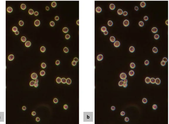
Figure 5.15. Resulting masks from applying two different ScerevisiCounter final versions to three sets of cells. The masks above are the result of the implementation of Version 2, while the masks below are the result of applying the Version 3. The images above correspond to the same images directly below these. The red manually defined borders are also visible. ... 94

Figure A.1. M_001 results. ... 105

(17)

Figure B.1. M_028 area results. Unsharp Mask radius equal to 1 pixel. ... 115

Figure B.2. M_028 area results. Unsharp Mask radius equal to 2 pixels. ... 115

(18)

Figure C.1. M_029 area results. Unsharp Mask radius equal to 1 pixels. ... 123

Figure D.1. M_030 area results. Unsharp Mask radius equal to 1 pixels. ... 131

(19)

Figure E.1. M_031 area results. Unsharp Mask radius equal to 1 pixels. ... 139

Figure E.3. M_031 area results. Unsharp Mask radius equal to 3 pixels ... 139

(20)

Figure F.1. M_032 area results. Unsharp Mask radius equal to 1 pixels. ... 147

Figure G.1. M_033 area results. Unsharp Mask radius equal to 1 pixels. ... 155

(21)

Figure I.1. N-Hefe_400x_dark-field_1 (Image 1 ). ... 177

Figure I.2. P hefe 800ms DF 400 (Image 2 ). ... 178

Figure I.3. P hefe 1200ms DF 400 (Image 3 ). ... 178

Figure I.4. N_Yeast 400x DF 300ms (Image 4 ). ... 179

Figure I.8. N Hefe 100ms (Image 8 ). ... 181

Figure I.10. N Hefe 200ms 2 (Image 10 ). ... 182

Figure I.13. Bild_227 (Image 13 ). ... 183

Figure I.17. 1B 1_100 (Image 17 ). ... 185

Figure I.18. 1CV1 1_10 (Image 18 ). ... 186

Figure I.19. 1N 1_100 (Image 19 ). ... 186

Figure I.20. 1P 1_100 (Image 20 ). ... 187 Figure J.1. Resulting mask from the sum of masks from experiments M_032_1, M_032_3 and M_031_4 with mask radius and weight equal to 2 pixels and 0.9, respectively, and experiment

(22)

M_031_2, with mask radius and weight equal to 3 pixels and 0.9, respectively. All experiments were performed with Image 2. ... 189 Figure J.2. Resulting mask from the sum of masks from experiments M_031_1 and M_031_2, with mask radius and weight equal to 3 pixels and 0.9, respectively, and experiments M_031_3 and M_030_4, with mask radius and weight equal to 2 pixels and 0.9, respectively. All experiments were performed with Image 2. ... 190 Figure J.3. Resulting mask from the sum of the masks in Figures J.1 and J.2. ... 190 Figure J.4. Resulting mask from the sum of masks from experiments M_029_4, M_030_2, M_031_1 and M_031_3, with mask radius and weight equal to 2 pixels and 0.9, respectively. All experiences were performed with Image 3. ... 191 Figure J.5. Resulting mask from the sum of masks from experiments M_031_1 and M_031_2, with mask radius and weight equal to 3 pixels and 0.9, respectively, and experiments M_031_3 and M_030_4, with mask radius and weight equal to 2 pixels and 0.9, respectively. All experiments were performed with Image 3. ... 191 Figure J.6. Resulting mask from the sum of the masks in Figures J.4 and J.5. ... 192 Figure J.7. Resulting mask from the sum of masks from experiments M_033_1, M_033_3, M_033_4 and M_031_2, with mask radius and weight equal to 2 pixels and 0.9, respectively. All experiments were performed with Image 4. ... 192 Figure J.8. Resulting mask from the sum of masks from experiments M_031_1 and M_031_2, with mask radius and weight equal to 3 pixels and 0.9, respectively, and experiments M_031_3 and M_030_4, with mask radius and weight equal to 2 pixels and 0.9, respectively. All experiments were performed with Image 4. ... 193 Figure J.9. Resulting mask from the sum of the masks in Figures J.7 and J.8. ... 193 Figure J.10. Resulting mask from the sum of masks from experiments M_033_1, M_032_2, M_032_3 and M_031_4, with mask radius and weight equal to 2 pixels and 0.9, respectively. All experiments were performed with Image 5. ... 194 Figure J.11. Resulting mask from the sum of masks from experiments M_031_1 and M_031_2, with mask radius and weight equal to 3 pixels and 0.9, respectively, and experiments M_031_3 and M_030_4, with mask radius and weight equal to 2 pixels and 0.9, respectively. All experiments were performed with Image 5. ... 194 Figure J.12. Resulting mask from the sum of the masks in Figures J.10 and J.11. ... 195

(23)

Figure J.13. Resulting mask from the sum of masks from experiments M_032_1, M_031_2 and M_032_3, with mask radius and weight equal to 2 pixels and 0.9, respectively, and experiment M_030_4, with mask radius and weight equal to 4 pixels and 0.9, respectively. All experiments were performed with Image 6. ... 195 Figure J.14. Resulting mask from the sum of masks from experiments M_031_1 and M_031_2, with mask radius and weight equal to 3 pixels and 0.9, respectively, and experiments M_031_3 and M_030_4, with mask radius and weight equal to 2 pixels and 0.9, respectively. All experiments were performed with Image 6. ... 196 Figure J.15. Resulting mask from the sum of the masks in Figures J.13 and J.14. ... 196 Figure J.16. Resulting mask from the sum of masks from experiments M_032_1, M_031_2 and M_032_3, with mask radius and weight equal to 2 pixels and 0.9, respectively, and experiment M_030_4, with mask radius and weight equal to 4 pixels and 0.9, respectively. All experiments were performed with Image 7. ... 197 Figure J.17. Resulting mask from the sum of masks from experiments M_031_1 and M_031_2, with mask radius and weight equal to 3 pixels and 0.9, respectively, and experiments M_031_3 and M_030_4, with mask radius and weight equal to 2 pixels and 0.9, respectively. All experiments were performed with Image 7. ... 197 Figure J.18. Resulting mask from the sum of the masks in Figures J.16 and J.17. ... 198

(24)

(25)

List of tables

Table 3.1. Object counting example results. ... 32 Table 4.1. Constitution of the experiments based on the groups. ... 61 Table 4.2. Configuration of Group 1 experiments. ... 62 Table 4.2. Configuration of Group 1 experiments (continuation). ... 62 Table 4.2. Configuration of Group 1 experiments (continuation). ... 62 Table 5.1. S. cerevisiae images title and receiving date. ... 68 Table 5.2. Group 1 experiments maximum results (/pixels). ... 69 Table 5.3. Number of True Areas with percentage below 95% of detected area. ... 72 Table 5.4. Results from different combinations of Convert 32 and Split Channels. ... 74 Table 5.5. Frequencies of mask weight values that generate an increase in the detected area. . 81 Table 5.6. Group 2 experiments maximum areas. ... 85 Table 5.7. Image 2 and Image 3 maximum areas. ... 88 Table 5.8. Image 4 and Image 5 maximum areas. ... 89 Table 5.9. Image 6 and Image 7 maximum areas. ... 90 Table 5.10. Final versions results on cell counting and area detection. ... 95 Table 5.11. Automatic vs manual cell count. ... 97 Table H.1. M_028_1 results. ... 163 Table H.2. M_028_2 results. ... 164 Table H.3. M_028_3 results. ... 164 Table H.4. M_028_4 results. ... 165 Table H.5. M_029_1 results. ... 165 Table H.6. M_029_2 results. ... 166 Table H.7. M_029_3 results. ... 166 Table H.8. M_029_4 results. ... 167 Table H.9. M_030_1 results. ... 167 Table H.10. M_030_2 results. ... 168 Table H.11. M_030_3 results. ... 168 Table H.12. M_030_4 results. ... 169 Table H.13. M_031_1 results. ... 169

(26)

Table H.14. M_031_2 results. ... 170 Table H.15. M_031_3 results. ... 170 Table H.16. M_031_4 results. ... 171 Table H.17. M_032_1 results. ... 171 Table H.18. M_032_2 results. ... 172 Table H.19. M_032_3 results. ... 172 Table H.20. M_032_4 results. ... 173 Table H.21. M_033_1 results. ... 173 Table H.22. M_033_2 results. ... 174 Table H.23. M_033_3 results. ... 174 Table H.24. M_033_4 results. ... 175

(27)

1. Introduction

This chapter aims to contextualize the reader to the subject of this work. Also the overall objectives of the dissertation are presented, as well as an outline of how the chapters are organized.

1.1. Motivation

The yeast Saccharomyces cerevisiae is one of the most important microorganisms employed in industry. S. cerevisiae size and shape distributions are affected by growth rate, mutation, and environmental conditions (composition, temperature, pressure, presence of oxidant agents, etc). S. cerevisiae cells have a round morphology with a size that may vary between 4 and 10 micrometers in diameter. Also have a division process known as budding. Budding is a form of asexual reproduction in which the original cell divides into “mother” and “daughter” cells. This project intends to classify S. cerevisiae morphology using microscopy and image analysis.

Image analysis is the process of extracting useful data directly from images by a computer or other device. Applications of image analysis are found in several areas of science and industry. A specialized image processing program using ImageJ will be developed to count cells and determine size fractions of various groups (small, large, budding).

ImageJ is a public domain Java image processing program [1]. Wayne Rasband, the core author of the program, designed it with an open architecture that provides extensibility via add-on programs written in Java (plugins) or in ImageJ´s programming language (macros). An ImageJ user has the four essential freedoms defined by Richard Stallman in 1986:

• The freedom to run the program, for any purpose.

• The freedom to study how the program works, and change it to make it do what you

wish.

• The freedom to redistribute copies so you can help your neighbour.

• The freedom to improve the program, and release your improvements to the public, so

that the whole community benefits.

1.2. Objectives

(28)

• Various groups of cell sizes and budding cells are counted automatically;

• The true cell size shall be estimated in order to group the cells into the right size group; • Budding cells have to be distinguished from overlapping cells and should not be

separated into mother and bud;

• As yeast cells do not appear with a clear black contrast in the microscope images,

probably a custom shape recognition algorithm has to be created;

• Cell morphological parameters, as well cell counting and cataloguing should be returned

as results;

• Background noise should not cause artefacts;

• Error handling routine: Information to the user, if the image cannot be analysed. What is

the reason? E.g.: Wrong magnification, dirty objective, too few/many cells, etc.

1.3. Dissertation structure

This dissertation is organized into six chapters. These are oriented to present the collected information during the investigation of the state of the art of the main topics underlying the dissertation and to present all steps taken for the development of an efficient plugin for processing and analysis of S. Cerevisiae images.

In Chapter 1, it is intended to guide the reader to the subject of this work, presenting the context and motivations to perform this work. The general objectives of the dissertation are also described.

Chapter 2 constitutes a literature review on the main themes of this work. A short description of Saccharomyces cerevisiae microorganism is performed, covering general aspects relating to its industrial applicability history, cell cycle and morphological aspects. Concepts of image processing and analysis are also given. Both sets of image analysis and processing techniques are distinguished with some examples of the most used and known methods. Moreover, the process of acquisition and sensing is also displayed in more detail as well as some work performed on the processing and analysis of S. cerevisiae microscopic images.

Next, the software for image processing – ImageJ – is described in Chapter 3 showing some processing techniques included in the program. It is also described in more detail the cell counting process program presented in the program. In addition, the program API classes and some examples of plugins coding are presented.

(29)

The methodologies and algorithms implemented in this work are presented in Chapter 4. It is explained the progress of the plugin code mainly the evaluation of the methods included. Also, the program body, referred as the Main Pipeline, is described and justified.

Chapter 5 presents and discusses the evolution of the image processing techniques and the experiments performed to obtain the final code version. Also, results of manual and automatic classification and counting of S. cerevisiae cells are compared.

Finally, Chapter 6 contains the most relevant conclusions as well as some perspectives for further work.

(30)

(31)

2. Context

In this chapter, the theoretical concepts which will serve as basis for the execution of this work are presented.

A brief description of global aspects of the yeast Saccharomyces cerevisiae focusing on aspects of their life cycle and morphology is given. First, a history context will be introduced followed by the description of it cell cycle presenting some of the processes occurring in the cell that leads to its division and duplication (replication). Next, some aspects concerning S. cerevisiae cells morphology will be presented, focusing on all aspects and shapes that this unicellular organism may adopt during their division phase (budding).Then the concept of image processing and analysis is presented. A brief introduction to digital images acquisition and sensing system will be taken. Subsequently, image processing and analysis techniques will be distinguished and some examples are presented. A short presentation of some practical cases of image analysis of S. cerevisiae cells is also presented.

2.1. Saccharomyces cerevisiae

Saccharomyces cerevisiae is a well-known, non-pathogenic, unicellular yeast (diameter usually vary between 4 and 10 µm). Its use dates back to ancient times which appear associated with processes like vinification, brewing and baking in ancient Egypt, Sumeria, Babylonia and Georgia. It is of main knowledge that its first appearance dates back to 1680 when van Leeuwenhoek using his primitive microscope saw yeast flocs fermenting wort [2]. However, it is only in the 19th

century that it is associated with the alcoholic fermentation. Then, the name Saccharomyces cerevisiae is assigned due to its connection with beer production. The genre name, derived from Latinized Greek, means “sugar fungus” and cerevisiae means beer in Latin.

Due to their unique advantages like being single celled; can be easily cultured; have capacity to grown readily in any type of bioreactor; having, more lately, its genome completely sequenced and etc, S. cerevisiae has received increasing attention since the early days of laboratory research. During the last 60 years, this yeast became one of the most studied organisms in the world, where its genetics, molecular biology, and metabolism have been studied extensively, as well its “cousin”, the bacteria Escherichia coli. Nowadays, this biological system is one of the preferentially election for molecular biotechnologists for high yield and quality of the final product.

(32)

One of these tasks is the synthesis of functioning recombinant proteins, by engineered S. cerevisiae cells as expression systems. In other cases, the genetically modified yeast itself is the desired product [3]. Furthermore, yeast is probably the most widely used unicellular eukaryotic organism in large-scale production of chemicals, pharmaceuticals, proteins, alcoholic beverages and bread [4].

2.1.1. Cell cycle

One of the most interesting aspects of S. cerevisiae life cycle is perhaps its ability to alternate between eukaryotic haploid (16 chromosomes) and eukaryotic diploid (32 chromosomes). But first, is also important to refer the two existing different types of haploid cells, denominated by a

and α mating types. The difference between cell types is found only at the genetic material level,

where at certain sites of the genome (MAT locus) can be inserted silent genes (genes of the genome which are not expressed) a and α. When located in the MAT locus, the function of these

genes is to regulate the production of the major contributor for the mating process, the proteins factor a and factor α. These hormones bind to cells of opposite mating and promote changes in

their cell surface so that fusion can take place. These different mating types of cells show primitive aspects of sexual differentiation. Furthermore, S. Cerevisiae cells can switch between a

and α type through a reversible mechanism known as cassette mechanism [5].

When two different haploid cells merge through the process called matting, new combinations of chromosomes are produced by genetic recombination yielding a diploid cell of a/α type, which

are incapable of mating with other cells. Mating of haploid cells yields diploid cells and meiosis of diploid cells produces a structure called ascus with four haploid products within, the gametes. Digestion of the ascus releases the four haploid meiotic products (ascospores) which, after germination, become haploid yeast cells again [4]–[6].

As well as many species of fungus and most of the microorganisms, in addition to the undifferentiated sexual reproduction, yeasts also reproduce asexually. All cell types (a, α and a/ α) are capable of proliferating by mitosis. According to Herskowitz [6] given sufficient nutrients,

the number of yeast cells doubles at approximately 100 minutes. During the cell cycle, the genetic material of the mother cell is duplicated and distributed by each mother cell and daughter. Unlike the classical process of cellular division in which a cell enlarges and divides by cell fission, yeast grows through a process referred to as budding. In this case, a daughter cell appears as a protuberance (bud) grows in the mother cell wall. Usually the mother cell is greater

(33)

than the daughter cell, and this need to increase in size in order to start the process of duplication of chromosomes. At some point, when the bud reaches a certain size, the previously replicated genetic material migrates to the daughter cell. After that, the disconnection of the bud from its mother cell takes place producing a characteristic bud scar on the wall of each cell [7]. Chant and Pringle [8] state that the site where the bud appears is different between haploid and diploid cells. In the first case, the formation of new buds follow an axial pattern, while in the second case both cell poles are potential bud sites. Another study aimed at identifying nonessentials genes involved in bipolar budding [9]. Through the analysis of bud scars on 127 mutants of yeast, three types of phenotypes were identified: unipolar, axial-like, and random. The life cycle of eukaryotic cells is usually divided into four phases: first gap phase (G1 phase), synthesis phase (S phase), mitosis phase (M) and second gap phase (G2 phase) (Figure 2.1 [10]). If left without nutrients the proliferation is abandoned at G1 phase resuming growth when nutrients become available again [6], [11].

2.1.2. Morphology

Many of the existing studies on S. cerevisiae fall into the mechanisms of how cells morphology is regulated and protein localization [9], [11]–[14]. Researchers had focused their interest in know specific morphologic characteristics of cells such as cell size, roundness, bud neck, and position. In the past, these studies were made by manually analysing images from microscopy. Nowadays, the reduction of these activities time is one of the main reasons for developing programs which automatically acquire information from images of microorganism’s cells.

Yu et al. [15] designed and developed a classification algorithm that is able to distinguish the

Figure 2.1. Schematic diagram for cell morphological changes used in cell cycle description (S phase: plaque duplication; G2 phase: nuclear migration; M phase: nuclear division; G1 phase: bud detachment) [10].

(34)

yeast cells in different phases of the cell cycle through image analysis. After a set of operations, the classifier distinguished between non budding cells, small bud and large bud cells which were associated to cell cycle phases G1, S and G2/M, respectively.

Saito et al. [16] presented the S. cerevisiae Morphological Database (SCMD), providing data related to yeast cells morphology in different stages of the cell cycle and information about the location of nuclear DNA and actin (http://yeast.gi.k.u-tokyo.ac.jp/datamine/). The authors developed a program for automatic image analysis [17] and analysed thousands of micrographs of yeast mutant cells and results were stored at SCMD. In addition, the database allowed the user to find similar yeast mutants in a particular number of morphological features, through a query search. The cell shape parameters recognized by the program were: long axis length; mother cell and bud roundness (long axis length / short axis length), bud neck position angle, bud growth direction angle, and the fitness value that showed how the cell line fits to the ellipse. The program was also able to quantify more 501 morphological parameters.

The Phenomics of yeast Mutants (PhenoM) is another database similar to SCMD [18]. In this database, morphological quantitative data acquired from 78194 morphological images of different yeast mutants are stored. In addition, characteristics obtained from other studies (bud size, cell area, roundness and etc), temperature data, cellular components of 775 yeast mutants, as well as other 865 morphological parameters are also presented. The database also provided several data-mining tools including a module for phenotypic comparison between mutant strains and a Gene Ontology module for functional enrichment analysis of gene sets showing similar morphological changes.

The Yeast Resource Center Public Image Repository (YRC PIR) is a large database of S. cerevisiae and Schizosaccharomyces pombe cell images (http://images.yeastrc.org) depicting the subcellular localization and colocalization of proteins [19]. The user can select one or more of 1259833 stored TIFF (Tagged Image File Format) images, by searching the data according to a set of experimental options, such as: data source; number of channels; number of z-sections; number of time-series; objective; binning; image size, and also according to a set of biological options, namely: proteins of interest and selected strain of the available species.

One of the most important aspects of yeast cell morphology is perhaps the size of the bud. Usually, a distinction is made according to bud size groups, including: no bud; small bud; medium bud and large bud. Each one of the categories may be associated to a range of possible mother and bud cell sizes ratio values. Another set of parameters important to mention is the cell

(35)

shape parameters. Figure 2.2 displays some of these features. It should be noted that all these parameters do not take into account the three-dimensional plane of the cells and that sometimes another possible morphological configuration could be presented. These configurations, such as elongated cells, mother cells with more than one bud, fusing haploid cells during the mating process as well the presence of diploid buds during a specific process, are called complexed cells. Complexed cells may appear in certain conditions of stress. Furthermore, Zalewski and Buchholz [20] categorized the cells of yeast in four distinct groups according to the morphology: (1) proportion of single cells with bud, (2) complexed cells with two or more cells of identical size, (3) single cells with large vacuole, and (4) dead cells, indicating the culture growth phase and the nutrient richness of the medium.

2.2. Image processing and analysis

Image analysis and processing is the extraction of quantitative and qualitative information from images by appropriate techniques.

An image can be viewed as a set of distributed data in a lattice or array, with positions defined by a set of elements from the Cartesian plane (Figure 2.3 [21]). Thus, the data values could be described as a two-dimensional function, f (x, y), where x and y, coordinates of the Cartesian plane, assume integer values from 0 to N - 1 and M - 1, respectively, in images with size N × M.

(36)

Occasionally, images may be squares, making so, M equal to N. Another frequently used nomenclature is the given spaces generated by the intersection of rows and columns of a matrix. In this case, i and j represents the row and column numbers, respectively, within the same range of integer values, in a similar way, of the previous example. Each element composing this matrix, grid or lattice if preferred, is named by picture element, image element, pixel or pel, being pixel the best known denomination [21]. Data values, f, is a discrete representation of the intensity or amount of visible light (or any other radiation in the electromagnetic spectrum) reflected (or transmitted) by an object. High intensities are typically translated into a high, or near the maximum values, whereas is usually to translate low intensities into low, or near the minimum values. It should be noted that due to the reflective nature of the objects (the light is not totally reflect or absorbed by any physical object) as well as to image sensing and acquisition processes (described with more detail in the next chapter), the quantization does not distinguish between different colours of the visible spectrum (this is another area of image processing), but the intensity of the monochromatic light. Thus, the quantization of light can be achieved from a range of values, where white is represented by the maximum value and black represented by the minimum value, or vice versa. All intermediate values of this scale represent variations of the

0 y m -1

0 f_{(0, 0)} f_{(0, m-1)}

x f_(x,y)

(37)

monochromatic intensity. The most common scale used in this process is the grayscale. The intermediate values of the grayscale represent different intensities of gray – gray levels. Due to hardware considerations, the number of levels (L ) of the grayscale for quantifying the intensity is limited, taking integer values in the order of powers of 2:

𝐿𝐿 = 2𝑘𝑘 _(2.1)

The number of bits required to store a digital picture is:

𝑏𝑏 = 𝑀𝑀 × 𝑁𝑁 × 𝑘𝑘 _(2.2)

As may be seen from equation 2.2, the number of bits required for storing a digital image is proportional to k. Therefore, it is common to refer to images with 2k _{gray levels as a "k-bit} image". For example, the most popular types of images, 8, 16 and 32-bit, are images with 256, 65536 and 4294967296 gray levels, respectively. From this point of view, it becomes obvious the relationship between the size of the grayscale and the memory needed for storage. The image size, M × N, which best known and most used designation is spatial resolution, also influence the number of memory bits required to allocate an image [22].

The collection of significant information from images becomes a little more elucidated after being provided a detailed description of the concepts related to the composition of the image. With informatics background, an image is visualized as an array of integers, and the application of basic algorithms for array manipulation is a common practice. However, image processing and analysis needs several techniques available with the assistance of computer programs. Thus, it is possible to extract qualitative and quantitative information from images using mathematical theorems ranging from the most simple to the most complex. The results of applying these sets of techniques are commonly divided into quantitative and qualitative. For example, the groups of techniques, whose results are images, are classified as image processing techniques. Whereas in groups of techniques that extract information from the images by "making sense", similarly to what happens with the human eye shape, are classified as image analysis techniques. This definition was adopted by Gonzalez & Woods [22] which divided the sets of image manipulation operations, according to the type of result returned by them.

2.2.1. Image sensing and acquisition

An image recording device responsible for acquiring digital images for the purpose of computational processing is also referred to as image digitizer. In most cases, a camera is commonly used for image acquisition.

(38)

The principle of acquiring digital images is applicable to all different types of digitizers. A source of electromagnetic radiation continuously brightens a scene or object and is reflected (or transmitted such as in X-rays) and captured by a sensing material, responsible for transforming the intensity of incoming light into voltage. In the case of digital cameras, the sensor is in reality predominantly a set of sensors arranged in the form of a 2-D array. The output waveform is the response of the sensors and a digital quantity is obtained by digitizing its response. The signal produced by each sensor of the camera leads to the formation of an array of picture elements with values directly proportional to the intensity of light passing through the lens [23]. This involves two processes: sampling and quantization. Digitizing the coordinate values of each one of the sensors is called sampling while digitizing the amplitude values of the voltage waveform is called quantization.

Visible light, as well as any other radiation of the electromagnetic spectrum, vary continuously in terms of wavelength and frequency values, never ending abruptly in a band and starting in another. For example, in this way the sensed data contained in the output waveform could be represented in a graph f (x, y) versus x whose function is continuous, except perhaps in the coordinates corresponding to peripheral regions or boundaries of objects. Notice that the value of a coordinate of the Cartesian plane is set to 1 to make it possible to do a graphical representation of a row of the image of the scanned object. Equally spaced samples are collected along the coordinate varying then the value of the other variable. Such proceeding is called sampling. Sampling limitations are imposed by the number of sensors and by the number of variations of the fixed coordinate [22]. The resultant continuous value of the sampling process is associated to a discrete level of the color scale used. For example, in 8-bit images the value of light intensity is equally divided into 32 to 32 between the ranges from 0 to 255, corresponding to each one of these ranges of values, different intensities of gray of the grayscale. The process of discretization of the values of brightness is called quantization.

Figure 2.5 shows an example of the pixel values distribution in the first line of a picture of a cell colony. The original image is shown in Figure 2.4. In this case the values are already discretized (after quantization) within a range of values between 0 and 255 (8-bit). However, the curve of the continuous function is easily perceptible. It is noted that the peak values of the function corresponding to white dots in the image represent cells. The variability in the intensity of the peaks demonstrates the perceptibility of the cells in the image. The higher the peaks are the

(39)

more noticeable are the cells in the picture due to the contrast with the background, being this perceptibility reduced as the peaks size decreases.

2.2.2. Image processing techniques

The main objective of processing techniques resides essentially in obtaining an image by modifying or transforming an original image by the action of specific operators. These operators (T ) are applied directly on the values of certain pixels, f (x, y), resulting in a new pixel value with

Figure 2.4. Cell colony image (available at http://imagej.nih.gov/ij/images).

Figure 2.5. Plot of the first line (0 ≤ x ≤ 406 and y = 0) of a cell colony picture. The values, discretized to have a range corresponding to 8-bit images, demonstrate a good approximation of what would be the function curve for the values with continuous amplitude.

(40)

position coordinates x and y:

𝑔𝑔(𝑥𝑥, 𝑦𝑦) = 𝑇𝑇[𝑓𝑓(𝑥𝑥, 𝑦𝑦)] (2.3), or also on the values of pixels of entire regions including whether or not the value of the target

picture element, f. The shape and size of these areas may be diverse, ranging from the most direct, vertical, horizontal or diagonal neighbors, to a set of neighboring elements with radius of a specified number of times of the central member, and may assume the most varied formats, including square, round, diamond, elongated, etc.

For example, a processing operation that aims to enhance images with high amounts of dark pixels whose areas of interest are the clearest ones is creating the negative image. The negative transformation of an image is easily translated by the following expression:

𝑔𝑔(𝑥𝑥, 𝑦𝑦) = 𝐿𝐿 − 1 − 𝑓𝑓(𝑥𝑥, 𝑦𝑦) (2.4), whereas stated earlier, L is the level of grayscale image. Reversing the intensity levels of an

image is the same as the equivalent of producing a photographic negative. In Figure 2.6 is shown how this operation applied to all the picture elements of the cell colony causes an increase in the ease of cells viewing.

This type of operation is included in the group of operations that aims the image enhancement. There are other operations whose quality results vary according with the definition given by the user. Several methodologies such as power-law and log transformations, histograms processing,

Figure 2.6. Image of a cell colony (left picture) and their negative transformation (right picture) (available at http://imagej.nih.gov/ij/images). The transformation was possible using the Image Inverter plugin from software

(41)

filters, and also the combination of different enhancement methods can be found. Subsequently, image improvement thorough pre-processing techniques, it is common practice before separating objects from the background making image segmentation.

Image enhancement techniques arise frequently associated with tasks such as automated cell counting, cell size and morphology characterization, determination of cell content, determination and quantification of protein localization and many others [24]–[30].

Filters improve images through the application of changes on groups of pixels. These are efficient computational methods that have the aim of reducing the level of "noise" and to emphasize edges in images. Filters provide an improvement to visual interpretation of images and can be a precursor to subsequent digital processing techniques such as segmentation [21]. The filtering process consists essentially to move, pixel by pixel, the centre of a "mask" of variable size (usually 3 × 3 pixel region) changing the value of the centre pixel according to a relationship between the values of the remaining pixels covered by the mask. Within this type of process there are different filters. Smoothing filters are primarily used for noise reduction and blurring while sharpening filters are used with the goal of highlight fine detail in an image to enhance detail that was been blurred. In general, filtering of an image of size M × N with a filter mask of size m × n is given by the expression:

𝑔𝑔(𝑥𝑥, 𝑦𝑦) = ∑𝑎𝑎𝑠𝑠=−𝑎𝑎∑𝑏𝑏𝑡𝑡=−𝑏𝑏𝑤𝑤(𝑠𝑠, 𝑡𝑡)𝑓𝑓(𝑥𝑥 + 𝑠𝑠, 𝑦𝑦 + 𝑡𝑡) (2.5), where a = (m - 1) / 2, b = (n - 1) / 2, w (s, t) is a filter coefficient for the corresponding mask pixels coordinates s, t. In order to achieve a completely filtered image it is necessary to apply eq. 2.5 to each one of the pixels of the image. Two considerations must be taken when the centre of the mask reaches a pixel in the image border. One of them, called padding, is to add replicated rows and columns, or with pixel values of 0, while the other consists in prevents the filter to advance to outside the image.

Segmentation or thresholding is the separation of pixels in a given range of values from other pixels with a specific range of values, different from the previous one. In practice, segmentation is the separation of regions of pixels corresponding to objects or part of objects of interest from the rest of the image. Each pixel of the image is allocated to one of these regions or categories. Thresholding can be a very effective method of measuring disjunctive and complex characteristics of an image. However, it could make wrong assignments of pixels to distinguish and separate an area of interest. Thus, segmentation is typically considered a critical step in image analysis.

(42)

Segmentation is a process usually preceded of the image binarization. Pixels values below a certain value or range of values are set equal to zero, while the pixels values above assume the maximum grayscale value. Thus, the image becomes represented by white and black pixels. Another type of thresholding result is highlighted as selected area which falls into a determined range of pixel value. In this case, two limit values are selected.

Figure 2.7 shows the results of the cell colony image segmentation as well as the results of filtering the original image followed by its segmentation. A median filter with radius of 2 pixels (Fig. 2.7c) was applied to the original image, where a slight reduction of background noise as well as some general image blurring is observed. This can be visualized by the image

Figure 2.7. Binarization of the cell colony image without filtering and after filtering. Figure 2.7a is the original cell colony image. Figure 2.7b is the result of thresholding the image of Figure 2.7a at pixel value 171. The image of Figure 2.7c is the result of applying a 3x3 median filter to the image of Figure 2.7a. The image of Figure 2.7d is the result of thresholding the image of Figure 2.7c at pixel value 171. All filter and threshold operations were performed

(43)

segmentation after the thresholding at pixel value of 171. More visible black spots can be observed in Figure 2.7b when compared to Figure 2.7d. This shows that the filter applied had an effect of image blur resulting in a cleansing of the image noise and also of some cells. This is also corroborated by the analysis of the histograms of the pixels distribution.

In this manner, it is shown that the filter caused a decrease of the maximum value assigned to a pixel, and a decrease in the average of pixel values.

2.2.3. Image analysis techniques

Image analysis is a field of digital image manipulation that differs from image processing. The purpose of image analysis is to emulate human vision, including learning and be able to make decisions based on vision inputs [22]. This technique is also associated with a high level of digital imaging computerized processes. The level of processing involves the "making sense" of a recognized set of objects where cognitive functions normally associated with vision are applied. While the human vision system collects information in a qualitative way, image analysis extracts quantitative information from the data sets assembled in images.

It can be stated that this group of techniques have, or could have, images as inputs, but whose outputs are attributes of images and not images as what happens with the application of image processing techniques. Usually, image analysis techniques are applied to images resulting from processing techniques. The most common image analysis techniques are morphological analysis, measurements, recognition, representation and description. Segmentation could also be included in this group of techniques. As stated earlier, segmentation results in image partition into its objects or constituents. The recognition based on objects segmentation, like assigning a label (e.g. cells) to objects, could be included in the group of image analysis techniques.

Morphological analysis relies commonly on the geometric aspects of an object. The parameters related to objects morphology are diameter, area, number, perimeter length, width, eccentricity, roundness, extension, convexity, solidity and compactness [31], fitting perfectly in the area of microscopic images analysis of yeast cells, or any other microorganism.

Besides the most basic mathematical morphological operations, such as translation, reflection, complement and difference, three types of operations characterize the morphological analysis technique: operations for size and shape, operations for connectivity and operations for texture [21]. The morphological analysis described in this chapter is applicable to binary images, usually derived from thresholding.

(44)

Operations for size and shape are the most direct and easiest morphological operations to use and are related with the properties, local shapes and sizes of objects in images. The components of the images are affected by how the structural elements of this technique, usually disks or squares are accommodated. Afterwards, several morphological operators are briefly described: dilation, erosion, opening, closing, hit-or-miss transform, boundary extraction, region filling and connected components.

Dilation is the operation in which object boundaries are expanded according to a structural element. The central pixel of the structural element, generally smaller in number of pixels, cycles through all pixels of the target object resulting in a wider object. This increase in size is related to the number of pixels of the structural element which exceeds the limits of the target object when the center pixel reaches the edge of the target object.

Erosion is the opposite of dilation. This technique causes a contraction of the boundaries of an object in a similar manner to the dilation process. In this case, the object is "reduced" according to the shape and size of the structural element. Once the limit of this element reaches the boundary of the object, the pixels between the object boundary and the central pixel of the structural element “drop out” from the constitution of the object. Once the center of the structural element to pass through all the pixels of the target object that would result in a contraction limits.

Opening and closing are intrinsic to dilation and erosion techniques. The result of opening is the same as the result of erosion followed by dilation of an object, causing smoothed contours, broken narrows isthmuses and eliminated small islands and sharp peaks. In an analogous way, the result of closing is the same result of dilation followed by erosion of an object, causing smoothed contours, breaks and fused narrowed longed thin gulfs and eliminated small holes. Hit-or-miss transform is an iterative morphological shape detection tool. Actually, this operation involves a number of basic operations such as erosion, complement, intersection and difference. After a number of iterations where each of these techniques is implemented according to a specific mathematical equation, the final result includes the coordinates of the object of interest in the image.

Boundary extraction is a technique which returns a region of pixels corresponding to the boundary of an object of interest. The quality of the resulting boundary is related to the shape of the structural element since the result of this operation is equal to the difference between the original object and the same object after erosion.