Positively Curved Killing Foliations via Deformations

(1)

Universidade Federal de São Carlos

Centro de Ciências Exatas e Tecnologia

Programa de Pós-Graduação em Matemática

Positively Curved Killing Foliations

via Deformations

Francisco Carlos Caramello Junior

(2)

Universidade Federal de São Carlos

Centro de Ciências Exatas e Tecnologia

Programa de Pós-Graduação em Matemática

Positively Curved Killing Foliations

via Deformations

Francisco Carlos Caramello Junior

Supervisor: Prof. Dr. Dirk Töben

Co-supervisor: Prof. Dr. Luiz R. Hartmann Jr.

Dissertation submitted to PPGM/UFSCar as partial fulfillment of the requirements for the degree of Doctor of Science.

This version contains the corrections and modifications suggested by the doctoral com-mittee during the dissertation defense on March 22, 2018.

This work was supported by the Brazilian Federal Agency for Support and Evaluation of Graduate Education within the Brazilian Ministry of Education.

(3)

Caramello Jr., Francisco Carlos

Positively curved Killing foliations via deformations / Francisco Carlos Caramello Junior. --2018.

105 f. : 30 cm.

Tese (doutorado)-Universidade Federal de São Carlos, campus São Carlos,São Carlos.

Orientador: Dirk Töben. Coorientador: Luiz Roberto Hartmann Junior. Banca examinadora: Dirk Töben, Luiz Roberto Hartmann Junior, Marcos Martins Alexandrino da Silva, Llohann Dallagnol Sperança, Fernando Manfio. Inclui referências

(4)

(5)

Acknowledgements

I owe my deepest gratitude to my supervisor, Prof. Dirk Töben, for the cru-cial ideas, the many insightful suggestions and the essential contributions he gave to this work, for his patience, encouragement and continuous support towards my formation and for the friendship we ended up developing through this process. I am also thankful to my co-supervisor, Prof. Luiz Hartmann, for sharing expertise and valuable career advices and for the suggestions and constructive criticism that signiﬁcantly improved the ﬁrst drafts of this dissertation. I thank Prof. Marcos Alexandrino as well, for his genuine solicitude and friendly hospitality during my occasional visits to IME.

I am grateful to my ﬁancée, Thais, for keeping me such a sweet company through both the brightest and the darkest hours of these years, for the great adventures that we shared and are yet to share together and, above all, for the caring love that we sustain toward each other. I express here as well my profound gratitude to my mother, Adriana, for the unconditional love, the unceasing assistance and the moral guidance she always provided me. I also thank my other family members, for the support they gave me along the way, and my fellow doctoral students, for the cooperation, the stimulating discussions and, of course, all the fun we have had in these four years.

(6)

“Though this be madness, yet there is method in’t.”

(7)

Resumo

Mostramos que uma variedade admitindo uma folheação de Killing com cur-vatura seccional transversa positiva e defeito máximo se ﬁbra sobre quocientes ﬁni-tos de esferas ou espaços projetivos complexos com pesos. Este resultado é obtido deformando-se a folheação em uma folheação fechada enquanto preservamos pro-priedades geométricas transversas, o que nos permite aplicar resultados da geometria Riemanniana de orbifolds ao espaço das folhas. Mostramos também que a carac-terística de Euler básica é preservada por tais deformações, o que nos provê algumas obstruções topológicas para folheações Riemannianas.

Abstract

(8)

List of Figures

1.1 A foliation is locally deﬁned by submersions . . . 17

1.2 λ-Kronecker foliations . . . 18

1.3 The ﬂow of a foliate ﬁeld preserves the foliation . . . 19

1.4 Sliding along the leaves . . . 21

1.5 The1-dimensional foliations of S3 (via stereographic projection) . . . 25

1.6 The Molino construction . . . 30

1.7 The orbits of the Molino sheaf are the closures of the leaves . . . 32

2.1 The space W . . . 36

2.2 Homothetic transformation with respect toN . . . 41

3.1 A homothopic deformation . . . 47

3.2 Lift of γ to the Darboux cover . . . 48

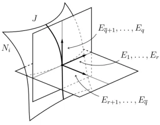
5.1 Construction of the vector ﬁeld W . . . 66

5.2 The frame E. . . 67

6.1 The holonomy groupoid . . . 80

A.1 TheZ3-Z4-football . . . 88

A.2 A smooth local lift . . . 90

A.3 Visualizing the stratiﬁcation ofCP3[λ] as a 3-simplex . . . 93

(9)

Introduction

The theory of foliations was initiated by H. Poincaré [Poi92] and I. Bendixson [Ben01] at the turn of the twentieth century, who studied the behavior of the so-lutions of first order ordinary differential equations on the plane. This theory was later developed and generalized to higher-dimensional systems by C. Ehresmann, G. Reeb, W. Thurston and many others, and nowadays accounts, via the Frobenius Theorem, for the qualitative behavior of first order partial differential equations on manifolds. Informally, a foliation is Riemannian if its leaves are locally equidis-tant. The precise definition involves the extra structure of a Riemannian metric that allows us to locally define the foliation as fibers of a Riemannian submersion. These objects, first presented by B. Reinhart [Rei59], are therefore approachable by the techniques of Riemannian geometry and form a very relevant class of foliations, whose research has been quite active since their introduction [see Ton97, Appendix D].

The structural theory for Riemannian foliations, due mainly to P. Molino, as-serts that a complete Riemannian foliation_F admits a locally constant sheaf of Lie algebras of germs of local transverse Killing vector ﬁeldsC_F whose action describes the dynamics of_F, in the sense that, for each leafLx ∈ F,

TxLx={Xx | X ∈(CF)x} ⊕TxLx,

where Lx denotes the closure of Lx (see Sections 1.7 and 1.8). From this it follows that the partition _F :={L | L∈ F} of M is a singular foliation, in the sense that

the dimension of the leaf closures may vary.

(12)

is, complete Riemannian foliations that have a globally constant sheaf C. In other words, if _F is a Killing foliation then there exists transverse Killing vector ﬁelds

X1, . . . , Xd such that TF = TF ⊕ hX1, . . . , Xdi. This class of foliations includes Riemannian foliations on simply-connected manifolds and foliations induced by iso-metric actions on compact manifolds.

In Chapter 1 we summarize the prerequisites from foliation theory used in this work. Chapter 2 contains some basic results and technical lemmas that are mostly direct generalizations of known results. In Chapter 3 we present the main tool for our study of Killing foliations: a deformation method that preserves transverse geometric properties of the foliation. Chapter 4 is dedicated to direct applications of this deformation technique. In Chapter 5 we study the behavior of the basic Euler characteristic, an algebraic invariant of a foliation, under such deformations. Finally, in Chapter 6 we use the deformation technique to obtain an obstruction for Riemannian foliations on manifolds with ﬁnite fundamental group and non-zero Euler characteristic. Appendix A surveys the basics of the diﬀerential geometry of orbifolds that we use.

Let us now introduce in more detail the main results obtained in this work. In the 1990s, K. Grove proposed that a classiﬁcation of Riemannian manifolds with positive sectional curvature and large isometry group should be pursued. Together with C. Searle, they introduced the symmetry rank as a way to interpret what it is meant by a “large” isometry group and showed in [GS94] that a closed Riemannian manifold with positive sectional curvature and maximal symmetry rank is diﬀeomorphic to either a sphere, a real or complex projective space or a lens space. A generalization of this result for Alexandrov spaces was obtained recently in [HS17]. We show the following transverse analogue of the Grove–Searle result.

Theorem A. Let F be a q-codimensional, transversely orientable Killing foliation of a compact manifoldM. If the transverse sectional curvaturesecF ofF is positive,

then

codim(F)_≥

codim(_F)₋1 2

(13)

Rieman-nian foliation_G such that M/_G is homeomorphic to either

(i) a quotient of a sphere Sq/Λ, where Λ is a finite subgroup of the centralizer of the maximal torus in O(q+ 1), or

(ii) a quotient of a weighted complex projective space _|CPq/2[λ]_|/Λ, where Λ is a finite subgroup of the torus acting linearly on CPq/2[λ] (this case occurs only whenq is even).

This is Theorem 4.4 in the text. We obtain the closed foliation_G by the already mentioned deformation technique that preserves some properties of the transverse geometry of_F, given by the result below.

Theorem B. Let (_F,gT₎ _{be a Killing foliation of a closed manifold} _M _satisfying

secF > c. Then there is a homotopic deformation of F into a closed Riemannian

foliation _G which can be chosen arbitrarily close to _F and satisfying secG > c.

Moreover, the deformation occurs within the closures of the leaves of F and M//G

admits an effective isometric action of a torus Td, where d = dim(C_F₍_M₎₎ _{is the}

defect of F, such that M/F ∼= (M/G)/Td_{. In particular,} _symrank(_G₎_≥_d_.

This result appears in the text as Theorem 3.5. The proof is based on a theorem by A. Haeﬂiger and E. Salem [HS90] that expresses _F as the pullback of a homo-geneous foliation on an orbifold. Theorem B enables us to apply results from the theory of Riemannian orbifolds to the study of Killing foliations, by passing from_F toM//_G. Besides Theorem A, another application of this technique is the following

“closed leaf” result, that generalizes [Osh01, Theorem 2] by allowing non-compact ambient manifolds. It is obtained by reducing the problem to an application of the Synge–Weinstein Theorem for orbifolds (Theorem A.14).

Theorem C. Let _F be an even-codimensional complete Riemannian foliation of a manifoldM satisfying|π1(M)|<∞. If secF ≥c >0thenF possesses a closed leaf.

A foliation _F on M deﬁnes a subcomplex of the De Rham complex of M that

(14)

the usual De Rham cohomology (see Section 1.4). In particular, consider χB(F) the basic Euler characteristic of_F, the alternate sum of the dimensions of the basic cohomology groups. We show that for a Killing foliation_F of a compact manifold this invariant localizes to the stratum Σdim(F) _{that consists of the closed leaves of}

F.

Theorem D. If _F is a Killing foliation of a closed manifold M, then χB(F) =

χ(Σdim(F)_/_F_).

Equivalently, using the language of transverse actions (see Section 1.8), we can write_F|_Σdim(F) =FgF, whereFgF denotes the ﬁxed-point set of the transverse action

of the structural algebra gF of F, so the formula in Theorem D becomes χB(F) =

χB(FgF), in analogy with the localization of the classical Euler characteristic to the ﬁxed-point set a torus action. Theorem D is a special case of a stronger result: we prove that

χB(F) =χB(F|Zero(X))

for any transverse Killing vector ﬁeld X ∈iso(F) (see Theorem 5.7).

Theorem D enables us to show that the basic Euler characteristic is preserved by the deformations devised in Theorem 3.5 (see Theorem 5.11). Using this we obtain the following transverse analogue of the partial answer to Hopf’s conjecture by T. Püttmann and C. Searle for manifolds with large symmetry rank [see PS01, Theorem 2], by reducing it to an orbifold version of this same result that we also prove (see Corollary 5.16).

Theorem E. Let _F be an even-codimensional, transversely orientable Killing foli-ation of a closed manifoldM. If secF >0 and

codim(_F)_≤ 3 codim(F)

4 + 1,

then χB(F)>0.

(15)

Theorem F. Let M be a closed manifold satisfying _|π1(M)| < ∞ and χ(M) 6= 0. Then any Riemannian foliation of M is closed.

This appears in the text as Corollary 6.5. It is shown in [Ghy84, Théorème 3.5] that a Riemannian foliation of a closed simply-connected manifoldM satisfying χ(M) ₆= 0 must have a closed leaf, a fact that also follows from the Poincaré-Hopf

(16)

Chapter 1 Preliminaries

For the reader’s convenience, in this chapter we collect some of the prerequisites on Riemannian foliations that will be used in this work. We assume the reader is familiar with the principal elements of the theory of smooth1 _{manifolds, as in}

[Lee13] or [War83] for example, Riemannian geometry, references being [Lee97], [Pet06] or [Sak97], and Lie group (actions) theory, as in [AB15], [Bre72], [DK00], and [War83]. We also assume some background in algebraic topology, for which we refer to [Hat02] and [Spa81], and sheaf theory language, that can be found in [Bre97]. The readers acquainted with the theory of Riemannian foliations, as presented in [MM03], [Mol88] or [Ton97], may skip this chapter probably without compromising the reading.

The brief exposition we do here follows mainly the references [Mol88], [MM03], [Ton97] and [Asa+14]. Further references are [CC00], [GW09] and [CN85].

1.1 Foliations

Let M be a smooth n-dimensional manifold. A foliation atlas of dimension

p_∈NforM is a smooth atlas_{φi :Ui →Rp×Rn−p}i∈I forM for which the changes of charts are locally of the form φij(x, y) = (φ1ij(x, y), φ2ij(y)), with respect to the decompositionRn=Rp_×Rn−p. EachUi is partitioned intoplaques, which are the

1

For us, “smooth” will always mean “of differentiability class C∞_{”. Also, we will often omit the}

(17)

connected components of the sets φ−_i 1(Rp _{× {}_y_}₎_{. These plaques glue together to} form immersed connected submanifolds ofM that we call leaves. The partition F

ofM into leaves is a (regular) foliationofM of dimensionp. We call q=n₋pthe

codimension of _F and, for x∈M, we denote the leaf containingx by Lx.

It is not diﬃcult to prove [see MM03, Section 1.2] that the following objects can be used as alternative deﬁnitions for _F.

• A smooth involutive distribution ∆of rankp ofT M. In this case∆x =TxLx.

• An integrable subbundle T_{F ⊂}T M of rank p, called thetangent bundleof

F. Here, of course, we have TxF =TxLx.

• A subsheaf of Lie algebras XF ⊂XM with constant span dimension p. In this case, for U _⊂M open, X_F(U)is the space of vector ﬁelds in U tangent to the

leaves. We denote XF(M) simply byX(F).

• A locally trivial diﬀerential graded ideal I_⊂Ω∗₍_M₎_{of rank}_q_{. Here, if}_U _⊂_M

is an open subset on which I is trivial, then I_|U is generated by q linearly independent 1-forms α1_{, . . . , α}q _and

TxLx = q \

i=1

ker(αi_x).

• An open cover{Ui}i∈I ofM, submersionsπi :Ui →Ui, withUi ⊂Rqopen, and diﬀeomorphismsγij :πj(Ui∩Uj)→πi(Ui∩Uj)satisfyingγij◦πj|Ui∩Uj =πi|Ui∩Uj

for all i, j ∈ I. The collection {γij} is a Haefliger cocycle representing F and each Ui is a simple open set for F (see Figure 1.1). We will assume without loss of generality that the ﬁbers π−_i 1(x) are connected.

Example 1.1. Let(M,_F) be a foliation andf :N _→M a smooth map transverse

to_F, that is, f is transverse to each leaf. Then f deﬁnes a foliationf∗₍_F₎_on_N _as

follows. If(Ui, πi, γij)is a cocycle representingF, thenf∗(F)is given by the cocycle

(Vi, π′i, γij), whereVi =f−1(Ui)andπi′ =πi◦f|Vi. Observe thatT f

∗₍_F_{) = d}_f−1₍_T_F₎

(18)

Ui

Uj

πi

πj

F

γji

Ui

Uj

Figure 1.1: A foliation is locally deﬁned by submersions

Example 1.2. Lie group actions constitute a main source of foliations. Precisely, recall that when µ : G×M → M is a smooth action, each orbit Gx is the image

of an injective immersion G/Gx → M [see, for instance, AB15, Proposition 3.14]. Thus, if we suppose that dim(Gx) is a constant function of x, it follows that the connected components of orbits of G decompose M into immersed submanifolds of

constant dimension. This decomposition _F is easily seen to be a foliation, because

Tx(Gx) = d(µx)e(g), so the ﬁeldsV∗ ∈X(M),V ∈g, induced by the action generate

TF, showing that this is an involutive distribution.

A speciﬁc example is the following. Consider the ﬂat torus T2 = R2/Z2. For

eachλ∈(0,+∞), we have a smooth R-action

R_×T2 _−→ T2

(t,[x, y]) _7−→ [x+t, y+λt]

with dim(R_[_x,y_]) ≡ 0. The resulting foliation is the λ-Kronecker foliation of the torus, _F(λ). Observe that when λ is irrational each leaf is dense in T2, while a

rational λ yields closed leaves (see Figure 1.2).

When a foliation _F is given by the action of a Lie group we say that _F is homogeneous.

(19)

irrational λ rational λ

Figure 1.2: λ-Kronecker foliations

B and T be smooth manifolds, let h : π1(B, x0) → Diff(T) be a homomorphism

and denote by ρ : Bb _→ B the projection of the universal covering space of B. On

f

M := T _×Bb, the ﬁbers of the ﬁrst projection Mf _→ T determine a foliation _Fe.

Deﬁne an action ofπ1(B, x0) onMfby setting, for [γ]∈π1(B, x0),

[γ]_·(t,ˆb) =h [γ]−1(t),ˆb_·[γ],

where ˆ_b_·_[_γ_] _{denotes the image of} ˆ_b _{by the deck transformation associated to} _[_γ_]_.

There is a manifold structure on M = M /πf 1(B, x0) [see Mol88, p. 28] such that

the orbit projection π : Mf → M is a covering map and, if τ : M → B is given

by τ(π(t,˜b)) = ρ(ˆb), then it is the projection of a ﬁber bundle with total space

M, base B, ﬁber T and structural group h(π1(B, x0)). The action of π1(B, x0)

preserves the leaves of _Fe, so projecting through π we obtain a foliation _F on M

withcodim(F) = dim(T), constructed by suspension of the homomorphismh.

For example, the Kronecker foliation_F(λ)(see Example 1.2) can be obtained by

the suspension of the homomorphismπ1(S1,1)∼=Z→Diff(S1)given byk 7→e−2πiλk.

As the Kronecker foliation shows, a leaf Lof a foliation _F need not to be closed

as a subspace of the ambient manifold M. We denote the set of leaf closures by

F := {L _| L _{∈ F}}. Understanding _F is part of the study of the dynamics of the

foliation. In the simple case when _F = F, that is, when all the leaves of F are

closed, we say that_F is a closed foliation.

(20)

Foliate Not foliate

Figure 1.3: The ﬂow of a foliate ﬁeld preserves the foliation

case, choices of orientations for T_F and ν_F give, respectively, an tangential ori-entation and a transverse orientation for _F. It is always possible to choose an orientable ﬁnite covering space Mc of M such that the lifted foliation _Fb is

trans-versely (and hence also tangentially) orientable [see CC00, Proposition 3.5.1]. In terms of a Haeﬂiger cocycle, _F is transversely oriented if and only if there is a cocycle _{(Ui, πi, γij)} representing F that satisﬁes det(dγij) > 0 as a function on

πj(Ui∩Uj), for all i, j ∈I.

Let(M,_F)and (N,_G)be foliations. Afoliate morphism between (M,_F)and (N,_G) is a map f : M _→N that sends leaves of _F into leaves of _G. When there is

such f, the foliations _F and _G are often said to be congruent. In particular, we

may consider_F-foliate diﬀeomorphismsf :M →M. The inﬁnitesimal counterparts

of this notion are the foliate vector fields of _F, that is, the vector ﬁelds in the subalgebra

L(_F) = _{X _∈X(M) _|[X,X(_F)]_⊂X(_F)_}.

If X _∈ L(_F) and π : U _→ U is a submersion locally deﬁning _F, then X_|U is π -related to some vector ﬁeldX_U ∈X(U). In fact, this characterizesL(F)[see Mol88,

Section 2.2]. Another characterization is that the local ﬂows of the ﬁelds in L(_F)

send leaves to leaves (see Figure 1.3).

The Lie algebra L(_F)also has the structure of a module, whose coeﬃcient ring

consists of the basic functions of _F, that is, functions f ∈ C∞₍_M₎ _{such that}

Xf = 0 for every X _∈ X(_F). We denote this ring by Ω0

(21)

through each submersionπ :U _→U locally deﬁning _F to a smooth function on the

quotient U [see Mol88, Section 2.1].

The quotient ofL(_F)by the idealX(_F)yields the Lie algebral(_F)of transverse vector fields. For X ∈L(F), we denote its induced transverse ﬁeld by X ∈l(F).

Note that each X deﬁnes a unique section of ν_F and that l(_F) is also a Ω0

B(F) -module.

1.2 Holonomy

Let (M,F) be a foliation represented by the cocycle {(Ui, πi, γij)}. The pseu-dogroup of local diﬀeomorphisms (see Section A.4) generated by γ = _{γij} acting on

Tγ := G

i

Ui

is the holonomy pseudogroup of _F associated to γ, that we denote by Hγ. If

δ is another Haefliger cocycle defining F then H_δ is equivalent to H_γ, so we can define, up to equivalence, the holonomy pseudogroup of_F. We will write(TF,HF)

to denote both this equivalence class and a speciﬁc representative in it, for it seldom leads to confusion. It is clear thatTF/HF is precisely the M/F ofF endowed with

the quotient topology.

Example 1.4. If (M,_F) is given by the suspension ofh:π1(B, x0)→Diff(T) (see

Example 1.3) we can choose a cocycle_{(Ui, πi, γij)}representing F where eachUi is the domain of a trivialization ofτ :M _→Bandπi :Ui →T is the trivial projection. Then H_F is just the pseudogroup generated by _h₍_π₁₍_{B, x}₀₎₎ _< _Diff(_T₎, encoding the recurrence of the leaves on T.

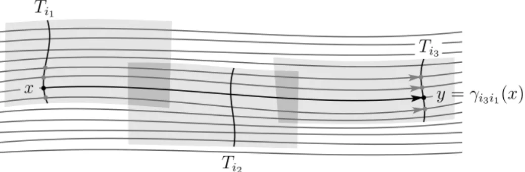
If L := Lx = Ly, choose a path c : [0,1] → L joining x to y. Fix a cocycle

{(Ui, πi, γij)} representing F and a subdivision 0 = t1 < · · · < tm+1 = 1 such that

s([tk, tk+1])⊂Uik for some Uik. Then, there is a diﬀeomorphism

γimi(m−1)◦γi(m−1)i(m−2)◦ · · · ◦γi2i1 =γimi1

(22)

y =γi3i1(x)

x Ti1

Ti2

Ti3

Figure 1.4: Sliding along the leaves

with a total transversal F_iTi for F containing x and y, this becomes the “sliding along the leaves” notion [Mol88, Section 1.7] (see Figure 1.4). Let us denote the germ of γimi1 at x by hc. This germ actually depends only on the ∂[0,1]-relative

homotopy class ofc[see CC00, Proposition 2.3.2], hence, if we consider in particular

the holonomy groupof L at x, that is, the group

Holx(L) ={hc |c: [0,1]→L is a loop},

we have a surjective homomorphismh:π1(L, x)→Holx(L).

As the isomorphism class of Holx(L) does not depend on x, we often omitx in this notation. In particular, we can say that L is a leaf without holonomy (or a generic leaf) when Hol(L) = 0. It follows immediately from the surjectivity of

h that simply-connected leaves are without holonomy. Also, it can be shown that

leaves without holonomy are generic, in the sense that _{x _∈ M _| Holx(L) = 0} is residual inM [see CC00, Theorem 2.3.12].

Leaf holonomy plays the same role of the stabilizer in the case of group actions. In particular, there is the following analogue to Proposition A.4 [see, for example, MM03, Theorem 2.15].

Proposition 1.5. Let _F be a q-codimensional foliation of M whose every leaf is compact and with finite holonomy. Then M/_F has a canonical q-dimensional orb-ifold structure. Relative to this structure, the local group of a leaf in M/_F is its holonomy group.

We will denote the orbifold obtained this way by M//_F in order to distinguish

(23)

(see Section A.3).

Note that if Holx(L) is ﬁnite it is possible to identify it with a subgroup of

Diff(T), where T is a small local transversal of _F passing through x. With this

in mind we can state the famous Reeb Stability Theorem as follows [see MM03, Theorem 2.9; CC00, Theorem 2.4.3]2_.

Theorem 1.6 (Generalized local Reeb stability). Let _F be a smooth foliation with a compact leafLx. If Holx(L)is finite then there is a saturated tubular neighborhood

pr : Tub(Lx) → Lx restricted to which F is congruent to the foliation given by the

suspension of h:π1(L, x)→Holx(L)<Diff(T), where T = pr−1(x).

In particular, for every y _∈ Tub(L) the projection pr : Ly → Lx is a ﬁnitely-sheeted covering map, the number of sheets being the index _|Holx(Lx) : Holy(Ly)|.

1.3 Foliations of Orbifolds

Let _O be an orbifold with atlas _A ={(Uei, Hi, φi)} and associated pseudogroup

(UA,HA) (see Appendix A). Following [HS90, Section 3.2], we deﬁne a smooth

foliation _F of _O as a smooth foliation of UA which is invariant by HA. The atlas

can be chosen so that on eachUei the foliation is given by a surjective submersion with connected ﬁbers onto a manifold Ti. The holonomy pseudogroup of F, therefore, will be generated by the local diﬀeomorphisms of the disjoint unionF_i_∈_ITi that are projections of elements of H_A.

1.4 Basic Cohomology

Let(M,_F) be a smooth foliation. A covariant tensor ﬁeldξ onM is _F-basic if

ξ(X1, . . . , Xk) = 0, whenever some Xi ∈ X(F), and LXξ = 0 for all X ∈X(F). In particular, we say that a differential formω _∈Ωi₍_M₎ _is _basic_{when it is basic as a} tensor field. By Cartan’s formula,ωis basic if, and only if, iXω= 0 andiX(dω) = 0 for all X_∈X(_F). These are the differential forms that project to differential forms

2

(24)

in the local quotients U and are invariant by the holonomy pseudogroup of _F [see

Mol88, Proposition 2.3]. We denote the Ω0

B(F)-module of basic i-forms of F by

Ωi

B(F). Then

Ω∗_B(_F) :=

q M

i=0

Ωi_B(_F)

is the_∧-graded algebra of basic forms of _F. By deﬁnition, Ω∗

B(F) is closed under the exterior derivative, so we can consider the complex

· · ·−→d Ωi_B−1(F)−→d ΩiB(F) d

−→Ωi_B+1(F)−→ · · ·d .

The cohomology groups of this complex are the basic cohomology groups of _F, that we denote by Hi

B(F). A foliate map f : (M,F)→(N,G)pulls basic forms on

N back to basic forms onM and hence induces a linear mapf∗ _:_Hi

B(G)→HBi(F). We deﬁne, when the dimensions dim(Hi

B(F)) are all ﬁnite, the basic Euler characteristicof _F as the alternate sum

χB(F) = X

i

(₋1)idim(H_Bi(_F)).

In analogy with the manifold case, we say thatbi

B(F) := dim(HBi (F))are thebasic Betti numbers of _F. When _F is the trivial foliation by points we recover the classical Euler characteristic and Betti numbers of M.

Since we have an identification between _F-basic forms and H_F-invariant forms on TF and an identification between differential forms on an orbifold O and HO

-invariant forms onUO, Proposition 1.5 gives us the following.

Proposition 1.7. Let (M,F)be a foliation such that every leaf is compact and with finite holonomy. Then the projectionπ :M _→M//_F induces an isomorphism of dif-ferential complexesπ∗ _{: Ω}∗₍_M//_F₎_→_Ω∗

(25)

1.5 Riemannian Foliations

Let _F be a smooth foliation of M. A transverse metric for _F is a symmet-ric, positive, _F-basic (2,0)-tensor ﬁeld gT _on _M_{. In this case} ₍_M,_F_,_gT₎ _{is called} a Riemannian foliation. On the other hand, a Riemannian metric g on M is

bundle-like for _F if for any open set U and any Y, Z ∈ L(F|U) perpendicular to the leaves we haveg(Y, Z)_∈Ω0

B(F|U). In this case, setting

gT(X, Y) := g(X⊥, Y⊥)

deﬁnes a transverse metric for _F, where we write X = X⊤ ₊_X⊥ _{with respect to}

the decomposition T M =TF ⊕TF⊥_{. Conversely, given} _gT _{one can always choose} a bundle-like metric on M that induces it [see Mol88, Proposition 3.3]. With a

bundle-like metric chosen, we will identify the bundles νF ≡TF⊥_.

Example 1.8. If a foliation _F on M is given by the action of a Lie group G (see

Example 1.2) and g is a Riemannian metric on M such that G acts by isometries,

then g is bundle-like for _F [see MM03, Remark 2.7(8)]. In other words, a foliation

induced by an isometric action is Riemannian.

Example 1.9. The1-dimensional Riemannian foliations of the euclidean sphereSn

where classiﬁed in [GG88, Theorem 5.4]. They exist only ifn is odd, sayn= 2k+ 1,

and are all homogeneous, given (up to isometric congruence) by R-actions of the

type3

t_·(z0, . . . , zk) = (e2πiλ0tz0, . . . , e2πiλktzk),

where λi ∈ (0,1]. In particular, such an action correspond to a closed riemannian

1-foliation F of Sn _{precisely when all} _λ

i are rational, say λi =pi/qi. Notice that in this case we can equivalently assume that λi ∈ N, by changing the parameter t to

lcm(q1, . . . , qk)t, henceSn//F =CPk[λ0, . . . , λk] (see Example A.5).

Let us visualize these foliations in the case of the 3-dimensional sphere, that

is, for k = 1. Consider the action of T2 ₌ _S1 _× _S1 _on _S3 _by ₍_t

0, t1)·(z0, z1) = (t0z0, t1z1). This action has two singular orbits, T2(1,0) and T2(0,1), that are

3

(26)

Figure 1.5: The1-dimensional foliations of S3 _{(via stereographic projection)}

diﬀeomorphic to S1. The other orbits are tori and coincide with the distance tubes

of the two singular orbits. The 1-dimensional Riemannian foliations of S3_{, up to}

congruence, can be identiﬁed with the1-dimensional Lie subalgebras ofR2 ∼= lie(T2)

via the induced action of the corresponding1-parameter subgroup. They restrict to

Kronecker foliations on each regularT2-orbit (see Figure 1.5).

Example 1.10. Let(T,g)be a Riemannian manifold. A foliationF deﬁned by the

suspension of a homomorphism (see Examples 1.3 and 1.4) h :π1(B, x0)→ Iso(T)

is naturally a Riemannian foliation [see also Mol88, Section 3.7].

It follows from the definition that gT _{projects to Riemannian metrics on the} local quotients Ui of a Haefliger cocycle {(Ui, πi, γij)} defining F [see Mol88, Sec-tion 3.2; MM03, Remark 2.7(2)]. The holonomy pseudogroup H_F then becomes a pseudogroup of local isometries of TF and, by choosing a bundle-like metric on M,

the submersions deﬁning _F become Riemannian submersions. We will say that _F has positivetransverse sectional curvaturewhen(TF,gT) has positive sectional

curvature. In this case we denote secF > 0. The notions of negative, non-positive

(27)

Example 1.11. By the description via Haeﬂiger cocycles, the pullback of a Rie-mannian foliation is obviously a RieRie-mannian foliation (see Example 1.1).

Bundle-like metrics can be characterized in terms of its geodesics [Rei59, see]. A metricg is bundle-like for(M,_F) if and only if a geodesic that is perpendicular to

a leaf in one point remains perpendicular to all the leaves it intersects. Moreover, he showed that geodesic segments perpendicular to the leaves project to geodesic segments in the local quotientsU. It follows that the leaves of a Riemannian foliation

are locally equidistant.

It is shown in [ASH85, Théorème 0] that the basic cohomology of Riemannian foliations on compact manifolds have ﬁnite dimension.

Theorem 1.12 (Alaoui–Sergiescu–Hector). Let _F be a Riemannian foliation of a closed manifold M. Then dim(Hi

B(F))<∞.

As remarked in [GT16, Proposition 3.11], the hypothesis that M is compact

can be relaxed toM/_F being compact, provided that_F is acompleteRiemannian foliation, that is,M is a complete Riemannian manifold with respect to some

bundle-like metric for_F. Hence, if this is the case, χB(F) is always deﬁned.

The following transverse analogue of the Bonnet–Myers Theorem due to J. Hebda will be useful [Heb86, Theorem 1].

Theorem 1.13 (Hebda). Let F be a complete Riemannian foliation satisfying RicF ≥c >0. Then M/F is compact and HB1(F)∼= 0.

1.6 Taut Foliations and Harmonic Forms

Another way to approach the basic cohomology of Riemannian foliations is via the basic laplacian ∆B [we refer to Ton97, Chapter 7, for an introduction]. Let F be a transversely oriented Riemannian foliation of a compact oriented manifoldM

(28)

adjoint of d with respect to _h·,_·i_B. We denote by _Hi

B(F) the space of harmonic basic i-forms, that is, basici-forms α satisfying ∆Bα = 0.

There is a version of the Hodge decomposition theorem for ∆B that gives an orthogonal decomposition Ωi

B(F) ∼= Im(d)⊕Im(δ)⊕ HBi (F) [see Ton97, Theorem 7.22] and provides an isomorphism Hi

B(F) ∼= HiB(F) [see Ton97, Theorem 7.51], which leads to duality theorems for the basic cohomology. Poincaré duality in its expected form, however, is only available for the so-called taut foliations, that we now introduce.

We say that a p-dimensional Riemannian foliation _F of M is taut when M

admits a metric for which all the leaves are minimal submanifolds4_{. Rummler’s}

criterion [see Rum79; or CC00, Theorem 10.5.9] characterizes tautness by the pres-ence of a form ω ∈ Ωp₍_M₎ _{such that} _ω_|

L is non singular for each leaf L ∈ F and

dω(Xi, . . . , Xp+1) = 0 whenever at least p of the vector ﬁelds Xi are tangent to

F. Another characterization is in terms of the vanishing of the cohomology class

of the mean curvature formκF ∈Ω1(M) [see Ton97, Chapter 3, for the deﬁnition].

Precisely, there is the following result5 _{by J. López [Lóp92, Theorem 6.4].}

Theorem 1.14 (López). A q-codimensional Riemannian foliation _F of a closed manifold is taut if and only if [κF] = 0. Moreover, when F is transversely oriented

it is taut if and only ifH_Bq(_F)₆= 0.

From the last part we see that tautness is necessary for Poincaré duality to hold on H∗

B(F). Basic Hodge decomposition arguments apply to this end, if this is the case, as was proved by F. Kamber and Ph. Tondeur [KT83] (with the additional hypothesis of orientability ofM) and later by A. Alaoui and G. Hector [AH86] and

V. Sergiescu [Ser85] (via homological techniques), giving us the following.

Theorem 1.15 (Kamber–Tondeur, Alaoui–Hector, Sergiescu). Let _F be a trans-versely oriented taut Riemannian foliation of codimension q of a closed manifold

M. Then Hi

B(F)∼=H q−i B (F).

4

This can be achieved with a bundle-like metric [see KT82, Corollary 2.31].

5

To apply López’s result directly to [κF], we observe that there is a bundle-like metric for F

for which the mean curvature form is basic [see Dom98] and that the class [(κF)B] of the basic

(29)

In particular, if codim(_F) is odd then χB(F) = 0. This, however, holds for any (not necessarily taut) odd-codimensional transversely oriented Riemannian fo-liation of a compact manifold, as shown by G. Habib and K. Richardson [see HR13, Corollary 3.3].

1.7 Molino Theory

Molino theory consists of structure theorems for Riemannian foliations developed by P. Molino and others in the decade of 1980. In this section we summarize it, following mostly the brief presentations in [GT16, Section 4.1] and [Töb14, Section 3.2]. A thorough introduction can be found in [Mol88].

Let (M,_F,gT₎ _{be a} _q_{-codimensional Riemannian foliation. Recall that} _gT in-duces a Riemannian metric π∗(gT) on the local quotient U of each foliation chart

(U, π). Consider the pullback to U of the Levi-Civita connection on U determined

this metric. By uniqueness, the pullbacks obtained this way glue together to a well-deﬁned connection _∇B _on _{T M}_{, the} _{canonical basic Riemannian connection,} where “basic” means that the local foliate ﬁelds in L(F|U) are parallel along the leaves with respect to_∇B_{. Note that} _∇B _{induces a covariant derivative on} _l₍_F|

U), that we also denote by _∇B_.

Let π _: _M

F → M be the principal O(q)-bundle of F-transverse orthonormal

frames6, which we call the

Molino bundleof _F. The normal bundleνF is

associ-ated toM

F and so the basic Riemannian connection∇B onνF induces a connection

formωF onMF. This connection form in turn deﬁnes an O(q)-invariant horizontal

distribution _H := ker(ωF) on M_F that allows us to horizontally lift the leaves of

F, deﬁning this way an O(q)-invariant foliation F of _M

F. By construction, ωF is

F-basic, that is, _i

X(ωF) = 0 and LXωF = 0 for allX ∈X(F), so we may regard

it as a mapωF :νF→so(q).

A practical way to think of _F is the following: if _x ₌ _π₍_x₎ and _y ₌ _π₍_y₎ 6

WhenF is transversely orientableM

F consists of twoSO(q)-invariant connected components

that correspond to the possible orientations. In this case we will assume that one component was chosen and, by abuse of notation, denote it also byM

F. Everything stated in this section then

(30)

theny belongs to the leaf _L

x ∈ F if and only if the orthonormal frame y of ν_yF

is the parallel transport of the frame x, with respect to _∇B_{, along some smooth} path inLx fromx toy.

We now deﬁne a transverse metric for_F. We lift the transverse metric_gT _on_ν_F to anO(q)-invariant metric on the O(q)-invariant transverse horizontal distribution

νH :=H/TF. The pullback₍_π₎∗_(gT₎ _{coincides with the pullback of the standard} scalar product on Rq by the fundamental 1-form θF : νF →Rq deﬁned by [see

Mol88, p. 70, p. 148]

θF(Xx) = (x)−1(dπ(X

x)),

wherex is an orthonormal basis of_ν

xF regarded as an isomorphismx :Rq →νxF andXx ∈ν

xF. Moreoverθ

F isF-basic [Mol88, Lemma 2.1(i)], so we get an F

-basic,O(q)-equivariant map ωF⊕θF :νF →so(q)⊕Rq. By the discussion above,

the pullback of the sum of an arbitrary (which is unique up to scalarλ) bi-invariant

scalar product onso(q)with the standard scalar product onRq byωF⊕θF yields an

O(q)-invariantF-transverse metric_(gT₎with respect to which_F is a Riemannian

foliation. Moreover,π _:_M

F →M becomes a transversely Riemannian submersion,

that is, dπ is surjective and restricts to an isometry _d_π _{: (}_ν_H₎

x →ν_xF for each

x_∈_M

F. We now ﬁxλby requiring that the ﬁbers ofπ satisfyvol((π)−1(x)) = 1.

The advantage of lifting _F to _F is that the latter admits a global transverse

parallelism, that is,ν_F is parallelizable by ﬁelds in_l₍_F₎[see Mol88, p. 82, p.148].

If we assume that_F is complete, then those ﬁelds admit complete representatives7 in

L(_F₎ [see GT16, Section 4.1]. Now, from the theory of transversely parallelizable

foliations, it follows that the partition _F of _M

F is a simple foliation, that is,

W :=M

F/Fis a manifold andFis given by the ﬁbers of a locally trivial ﬁbration

b: M

F →W [see Mol88, Proposition 4.1’], the basic fibration. Since F is O(q)

-invariant, by continuity so is _F, hence the action of _O(_q₎ on _M

F descends to an

action onW such that b is nowO(q)-equivariant. A leaf closure L∈ F is the image

by π of a leaf closure of _F, which implies that each leaf closure is an embedded 7

(31)

leaf closures

π

b

O(q)-orbits

O(q)b(x₎

O(q)b(y₎

x

Lx =Lx

Ly

x

L

x

(π₎−1₍_L y)

y

Figure 1.6: The Molino construction

submanifold ofM [Mol88, Lemma 5.1]8_{, that also corresponds to an}

O(q)-orbit inW.

This induces an identiﬁcation M/_{F ≡} W/O(q) and gives a commutative diagram

(see Figure 1.69₎

(M

F,F,O(q))

b _/

/

π

(W,O(q))

(M,_F) //M/F ≡W/O(q).

Fix L _{∈ F}, denote _J ₌ _L, consider the foliation ₍_J,_F_|

J) and deﬁne gF :=

l(_F_|

J). Then F|J is a complete Lie gF-foliation in the terminology of E. Fedida

[Fed71], whose work establishes that such foliations are developable, that is, they lift to simple foliations of the universal covering spaces [see Mol88, Theorem 4.1]. The restriction of _F to the closure of a diﬀerent leaf is isomorphic to ₍_J,_F_|

J), so gF is an algebraic invariant of F, called its structural algebra. We say that

d:= dim(gF) is the defectof F, motivated by the results in the next section.

8

Molino’s results are usually stated for a compact M, but completeness of _F is sufficient [see GT16, Section 4.1; Töb14, Section 3.2].

9

(32)

1.8 Molino Sheaf and Killing Foliations

Let (M,_F,gT₎ _{be a} _q_{-codimensional Riemannian foliation. A ﬁeld} _X _∈ _X₍_M₎ is a Killing vector field for gT _if _L

XgT = 0. These ﬁelds form a Lie subalgebra of L(_F) [see Mol88, Lemma 3.5] and there is, thus, a corresponding Lie algebra

of transverse Killing vector fields, that we will denote by iso(F,gT₎_{. We will} omit the transverse metric when it is clear from the context, writing just iso(_F).

Of course, these are the transverse ﬁelds that project to Killing vector ﬁelds on the local quotients of_F.

Now let (M,F,gT₎ _{be a complete Riemannian foliation. Consider on} _M

F the

sheaf of Lie algebrasC_F that, to an open set U⊂M

F, associates the Lie algebra

C_F(U) of the transverse ﬁelds in U that commute with all the global ﬁelds in

l(_F₎. Each ﬁeld inC_F(U)is the natural lift of a F-transverse Killing vector ﬁeld

onπ₍_U₎[see Mol88, Proposition 3.4]. The pushforward_π

∗(CF)will be called the

Molino sheaf10 _of

F, that we denote simply by C_F. From what we just saw, it is the sheaf of the Lie algebras consisting of the local transverse Killing vector ﬁelds that lift to local sections of C_F.

The sheafC_F is Hausdorﬀ [Mol88, Lemma 4.6] and its stalk₍C_F₎_x on each point is isomorphic to the Lie algebra g−_F1 opposed to g_F [Mol88, Proposition 4.4]. The

main motivation for the study of C_F is that its orbits describe the closures of the leaves of _F [Mol88, Theorem 5.2], in the sense that

{Xx | X ∈(CF)x} ⊕TxLx =TxLx.

Since C_F is locally constant, this means that for a small open set _U, ﬁxing a basis

X1, . . . , Xd for CF(U) we have T L|U =T L|U ⊕ hX1, . . . , Xdi for any L∈ F, where

X1, . . . , Xd∈L(F)are representatives for that basis (see Figure 1.7).

Using these facts one shows [see Mol88, Proposition 6.2] that _F is a singular Riemannian foliation, meaning that the module X(_F) of smooth vector ﬁelds

tangent to the leaf closures is transitive on each leaf closure (that is,_F is a singular

10

In Molino’s terminology this is thecommuting sheaf [Mol88], also sometimes referred to as

(33)

L U

Figure 1.7: The orbits of the Molino sheaf are the closures of the leaves

foliation in the terminology of H. Sussmann [Sus73] and P. Stefan [Ste74]) and that

M admits a Riemannian metric adapted to _F, that is, such that every geodesic that

is perpendicular at some point to a leaf closure remains perpendicular to every leaf closure that it intersects.

An interesting subclass of complete Riemannian foliations is the one consisting of foliations _F for which C_F is _globally constant. Such foliations will be called Killing foliations, following [Moz85]. In other words, if _F is a Killing foliation then there exists X1, . . . , Xd ∈ iso(F) such that TF = TF ⊕ hX1, . . . , Xdi. A complete Riemannian foliation is a Killing foliation if and only if C_F is globally

constant, and in this case C_F(M

F)is the center of l(F). Hence CF(M)is central

inl(F) (but not necessarily the full center) . It follows that the structural algebra

of a Killing foliation is Abelian, because we have g−_F1 ∼= C_F₍_M₎ ∼_{= (}C_F₎_x for each

x∈M.

Example 1.16. A complete Riemannian foliation_F of a simply-connected manifold is automatically a Killing foliation [see Mol88, Proposition 5.5], since in this case

C_F cannot have holonomy.

Example 1.17. Homogeneous Riemannian foliations provide another important class of examples [see Mol84, Lemme III]. In fact, if _F is a Riemannian foliation of a compact manifold M given by the action of H < Iso(M), then _F is a Killing

(34)

Speciﬁc examples in this class are, therefore, the λ-Kronecker foliations (see

Example 1.2) and the Riemannian 1-foliations of the round sphere (see Example

1.9).

Riemannian foliations deﬁned by the method of suspension11 _{are, in general, not}

Killing. A speciﬁc example can be seen in Example 4.2.

In the terminology of transverse actions introduced in [GT16, Section 2], a Killing foliation _F admits an eﬀective isometric transverse action of gF given by

the isomorphism gF ∋ V 7→ V ∗

∈ C_F₍_M₎ _< _iso₍_F₎, such that the singular fo-liation everywhere tangent to the distribution of varying rank gF· F deﬁned by

(gF·F)x := {V

∗

x | V ∈ gF} ⊕TxF is F [see GT16, Theorem 2.2]. For short, we write this as gF·F = F, that is, we denote by gF·F both the distribution and its

associated singular foliation.

11

(35)

Chapter 2 Transverse Killing Vector Fields and

the Structural Algebra

In this chapter we prove some basic facts about the zero sets of transverse Killing vector fields which will later be used in our study of Killing foliations. Although some of these results were not found in the current literature, they consist mainly of direct generalizations of known properties of Killing vector fields on Riemannian manifolds [see, for instance, Pet06, Chapter 7]. We also study the behavior of the structural algebra when a Riemannian foliation is lifted to a finitely-sheeted covering space.

2.1 Elementary Properties of Transverse Killing

Vec-tor Fields

Let us begin by establishing some notation. If (M,F,gT₎ _{is a Riemannian} fo-liation and X _∈ iso(_F,gT₎ _{is a transverse Killing vector ﬁeld (see Setion 1.8), we} denote by Zero(X) the set whereX vanishes, that is,

Zero(X) :=_{x_∈M _| Xx = 0}.

(36)

for any x _∈ U, the ﬁeld X_U is completely determined by (X_U)x and by the skew-symmetric linear map(∇U₍_X

U))x, where∇U is the Levi-Civita connection ofU [see, for example, Pet06, Propositions 27 and 28]. Hence it follows that, for anyx_∈ M,

the ﬁeldX ∈iso(F)is also uniquely determined by Xx and by the skew-symmetric linear map

(∇B_X₎

x :νxF →νxF,

where _∇B _{denotes the canonical basic Riemannian connection of} ₍_M,_F_,_gT₎ _(see Section 1.7).

We say that an _F-saturated submanifold N ⊂ M is horizontally totally geodesic if it projects to totally geodesic submanifolds in the local quotients U

of _F.

Proposition 2.1. Let(M,_F,gT₎_{be a Riemannian foliation and let}_X _∈_iso₍_F₎_{be a}

transverse Killing vector field. Then each connected component N of Zero(X) is an even-codimensional closed submanifold ofM saturated by the leaves of_F (and hence

F). Moreover, N is horizontally totally geodesic and if F is transversely orientable then (N,_F|N) is transversely orientable.

Proof. AsX is transverse, ifx∈Zero(X)thenLx ⊂Zero(X), hence each connected component N is saturated by leaves of _F. Furthermore, it is clear that Zero(X) is

closed, so Lx ⊂ Zero(X) and N is also saturated by the leaves of the singular foliation_F.

Letx∈N and let π :U →U be a local trivialization ofF with x∈U. IfX_U is

the Killing vector ﬁeld onU induced by X_|U, then

Zero(X)_∩U =π−1_(Zero(_X

U)).

In particular, N ∩U = π−1₍_N₎_{, where} _N _{is a connected component of} _Zero(_X

U). We know that N is a totally geodesic submanifold of U of even codimension [see

Kob72, Theorem 5.3] so, asπ is trivially transverse to N, it follows that N∩U is a

(37)

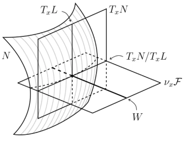
W

νxF

TxN

TxN/TxL

TxL

N

Figure 2.1: The space W

xtoyand a chain U =U1, U2, . . . , Uk ∋y of simple open sets coveringIm(γ). Then eachN ∩Ui is a horizontally totally geodesic submanifold and, as

N _∩(Ui∩Ui+1) = (N ∩Ui)∩Ui+1 = (N ∩Ui+1)∩Ui,

it follows thatdim(N∩U) = dim(N∩Uk). ThusN is a horizontally totally geodesic submanifold of M. Moreover, π is a Riemannian submersion, hence

codim(N) = codim(N _∩U) = codim(N)

is even.

It remains to show that if _F is transversely orientable then (N,_F|N) is also transversely orientable. Indeed,

(_∇BX)x :νxF →νxF

is skew-symmetric and vanishes on TxN/TxLx, so it preserves the gT-orthogonal complement (see Figure 2.1)

W =

TxN

TxLx ⊥

≤νxF.

Choosing the adequate orthonormal basis, (∇B_X₎

(38)

representa-tion of the type _          

0 α1

−α1 0

...

0 αl

−αl 0            ,

where l = dim(Wx)/2 = codim(N)/2. That is, Wx decomposes into 2-dimensional invariant subspaces Ej, j = 1, . . . , l. The eigenvalues ±iαj remain constant on N, because on each simple open setU _∋xthese are the eigenvalues of(_∇U₍_X

U))x, that are known to remain constant onN [see Kob72, p. 61]. Therefore we can decompose

the bundleW = (T N/T_F)⊥ _{into subbundles}

W =E1⊕ · · · ⊕El,

whereEj corresponds to the eigenvalue−α2j of(∇BX|W)2. Now deﬁne an endomor-phismJ of W by

J|Ej = 1

αj∇ B_X.

Then clearly J2 ₌ ₋_Id_{, so} _J _{deﬁnes a complex structure on} _W_{. In particular, we}

have thatW is orientable. As

T M T_F N

= T N

T_F ⊕W,

the result follows.

Recall that the symmetry rank of a Riemannian manifold is the rank of its isometry group. In analogy, if (M,F,gT₎ _{is a Riemannian foliation we deﬁne the} transverse symmetry rank of _F by

symrank(F) := max

a

n

dim(a)o,

wherearuns over all the Abelian subalgebras ofiso(_F). Fix a subalgebraa<iso(_F)

(39)

proper connected components of the zero sets of the transverse Killing vector ﬁelds ina. We have the following properties.

Proposition 2.2. For any N, N′ _{∈ Z}₍_a₎ _{the following holds:}

(i) Every transverse Killing vector field in a is tangent1

to N and, therefore, the restriction to N of the fields in a yields a commutative Lie algebra a_|N of

transverse Killing vector fields of_F|N.

(ii) If N is maximal in Z(a) with respect to set inclusion, then

dim(a_|N) = dim(a)−1.

(iii) Each connected component of N _∩N′ _{also belongs to} _Z₍_a_).

Proof. LetN andN′ _{be connected components of the transverse Killing vector ﬁelds}

X and X′ ina, respectively.

(i) Choose any Y ∈a. As we have that _LYX = [Y, X] = 0 and that Y ∈L(F) is a Killing vector ﬁeld for gT_{, it follows that}

0 = LYgT(X, X) =YgT(X, X)−2gT([Y, X], X)

= YkXk2

T.

That is, the ﬂow of Y preserves the level sets of _kX_k2

T and, hence, in particular, it preserves Zero(X). Therefore Y is tangent to N. It is now clear that a_|N is a commutative Lie algebra of transverse Killing vector ﬁelds of _F|N.

(ii) Suppose that N _{∈ Z}(a) is maximal and that Y _∈ a vanishes on N. Fix x_∈N and consider the commuting skew-symmetric applications

(_∇BX)x,(∇BY)x :νxF →νxF.

They both vanish on TxN/TxLx, so, again, as in the proof of Proposition 2.1, they preserve thegT_{-orthogonal complement} _W _{= (}_T

xN/TxLx)⊥ (see Figure 2.1), which

1

(40)

therefore decomposes as

W =E1⊕ · · · ⊕El, where2

l = dim(W)/2 and each Ei is a 2-dimensional subspace invariant by both

(_∇B_X₎

x and (∇BY)x. Now ﬁx any index i. As the space of skew-symmetric trans-formationsEi is one-dimensional, there exists some linear combination α(∇BX)x+

β(_∇B_Y₎

x that vanishes onEi. In particular,

ker(∇B₍_αX ₊_βY₎₎ x ⊃

TxN

TxLx ⊕

Ei

and, sinceker(_∇B₍_αX₊_βY₎₎

x completely determines the connected component of

Zero(αX+βY)containingx, it follows thatαX+βY vanishes on a set that contains N properly. This violates the maximality of N unless Y is a multiple of X, hence

dim(a_|N) = dim(a)−1.

(iii) Let C be a connected component of N _∩N′_{. First, by considering local}

trivializationsπ :U _→U of _F and observing that

N∩N′∩U = (N ∩U)∩(N′∩U) =π−1(N)∩π−1(N′) =π−1(N ∩N′),

whereN andN′ are connected components of the zero sets of the Killing vector ﬁelds

induced onU byX and X′ respectively, it follows as in the proof of Proposition 2.1

thatCis a submanifold, since each connected component ofN_∩N′ is a submanifold

of U [see Pet06, Proposition 30 (4)].

It is clear thatαX+βX′ vanishes onC for anyα, β _∈R. LetC′_{be the connected}

component of Zero(αX1 +βX2) containing C. For x ∈ C we have that the maps (_∇B_X

1)x and (∇BX2)x vanish simultaneously on

TxN

TxLx

∩

TxN′

TxLx

= TxC

TxLx

but not on any (nonzero) vector on the orthogonal complementW = (TxC/TxLx)⊥. Again, we decomposeW into 2-dimensional subspacesEi that remain invariant un-der both the commuting skew-symmetric maps(_∇B_X

1)x|W and (∇BX2)x|W. Since

2

(41)

these maps do not vanish simultaneously on the subspacesEi, it is possible to choose α, β ∈Rsuch that (∇B₍_αX ₊_βX′₎₎

x does not vanish onW. Hence

TxC′

TxLx

= ker(_∇B(αX+βX′))x

= TxC

TxLx

,

which shows thatC =C′_.

We end this section with a basic technical result that we will use later. Consider a Riemannian foliation_F of a closed manifoldM endowed with a bundle-like metric,

letX _∈iso(_F)and ﬁxN a connected component of Zero(X). Recall from

Proposi-tion 2.1 thatN is a compact submanifold, so it is known that for a suﬃciently small ε >0, if Bε(N) is the bundle of open balls consisting of vectors perpendicular toN and of length less than ε, then the restriction

exp⊥ :Bε(N)−→Tubε(N)

of the exponential map is a diffeomorphism onto a tubular neighborhoodTubε(N) ofN inM. If_kXxk=ε′ < εand y= exp⊥(Xx)then clearlyd(y, N) = ε. Moreover, the orthogonal projection πN : Tubε(N) → N is a locally trivial fibration whose typical fiber isπ_N−1(x) = exp⊥₍₍_B

ε(N))x). We will assume, decreasingε if necessary, that for eachy∈Tubε(N)the leaf Ly is transverse to πN−1(π(y)). The set of points

SN

ε′ in Tub_ε(N) which are at a distance ε′ from N is the tube of radius ε′ centered on N. It is precisely the image by exp⊥ _{of the bundle of spheres of radius} _ε′ _in

Bε(N), so it is a submanifold of M.

Let ηλ : T N⊥ → T N⊥ denote the product by a scalar λ > 0. Then on the union of the tubesSN

ε′ such thatλε′ < εwe deﬁne a homothetic transformation

hλ := exp⊥◦ηλ ◦(exp⊥)−1 of proportionality constant λ (see Figure 2.1). Lemma 2.3. With the notation above, πN and hλ are foliate maps.

Proof. Since_F is a singular Riemannian foliation and N is_F-saturated (see

Propo-sition 2.1), a geodesic perpendicular to N remains perpendicular to all the leaf

closures that it intersects, therefore if d(y, N) =ε′ _{it follows that} _T

(42)

N

Tubε(N)

SN λε′

SN ε′

hλ

Figure 2.2: Homothetic transformation with respect to N

leaf closure in _F (and hence any leaf of _F) intersecting Tubε(N) is contained in a tube centered onN.

Now letP be a relatively compact, connected, open neighborhood ofx=π(y)in

Lxand deﬁneTubε(P)andSεP′ just as we did forN. ThenTub_ε(P)is a distinguished tubular neighborhood, in the sense of [Mol88, p. 193]. By the same argument we gave above, we conclude that the connected componentPy ofLy∩Tubε(P)containing

y, called theplaqueof _F passing throughy inTubε(P), is entirely contained in SPε′ and, so, inSP

ε′ ∩SN_ε′, whereπ_P clearly coincides with π_N. Thus π_N maps plaques to plaques and is therefore foliate.

The proof that hλ is foliate consists of an adaptation of the proof of Molino’s homothetic transformation lemma [Mol88, Lemma 6.2], so we will just sketch it. It is suﬃcient to consider λ close to 1 so that yλ :=hλ(y) belongs to a distinguished neighborhood ofyand hence there are equidistant neighborhoodsΞ_∋yandΞλ ∋yλ inPy _and _Pyλ respectively, such that the shortest distance from a point _y′

λ ∈Ξλ ⊂

SN

λε′ to Ξ⊂ SN_ε′ is realized by the geodesic joining y_λ′ to its projection y′ in Ξ. But

d(y′_{, y}′

λ) = d(y, yλ) = ε′|1−λ| and such a distance between a point in SNε′ and a point in SN

(43)

2.2 The Canonical Stratification

As we already saw in the Sections 1.7 and 1.8, given a complete Riemannian foliation _F of M, the partition F deﬁned by the closures of the leaves of F is a

singular Riemannian foliation3 _of

M, whose dimension we deﬁne by

dim(F) = max

L∈F

n

dim(L)o.

We deﬁne the codimension of _F bycodim(_F) = dim(M)₋dim(_F). Notice that

the relationship between_F, the Molino sheafC_F and the structural algebra_g_F (see Section 1.8) enables us to write the defect of_F as

d= dim(gF) = dim(F)−dim(F) = codim(F)−codim(F).

Now for s satisfying dim(_F) _≤ s _≤ dim(_F), let us denote by Σs _{the subset of} pointsx_∈M such that dim(Lx) = s. Then we get a decomposition

M = [

x∈M

Σx,

called the canonical stratification of _F, where Σx is the connected component of Σs _{that contains} _x_{. Each component} _Σ

x is an embedded submanifold [Mol88, Lemma 5.3] called astratumof_F. Moreover, the restriction_F|Σx now has constant

dimension and forms a (regular) Riemannian foliation [Mol88, Lemma 5.3]. The

regular stratum Σdim(F) _{is an open, connected and dense subset of} _M_{, and each}

other stratum Σx 6= Σdim(F) is called singular and satisﬁes codim(Σx) ≥ 2 [see Mol88, p. 197]. In particular, codim (_F|Σx) < codim(F). The subset Σ

dim(F) _will

be called the stratum of the closed leaves, even though it is not, in general, a canonical stratum (for it can be disconnected).

Of course, the canonical stratiﬁcation is closely related to the structural Lie algebra gF. Consider F a q-codimensional Killing foliation of a closed manifold

M. W. Mozgawa shows in [Moz85, Théorème] that there are r = minL∈F{dim(L)}

3

(44)

vector ﬁelds in gF, linearly independent at every point of M, deﬁning a (q−r)

-codimensional foliation _F′ _of _M _{such that} _F′ ₌ _F and _F′ _{has at least one closed}

leaf. Whenr = 0 we also have the following.

Proposition 2.4. Let (M,_F) be a Killing foliation. Then there exists a transverse Killing vector field X ∈C_F₍_M₎ _{such that}

Zero(X) = Σdim(F).

Proof. Choose an enumerable cover{Ui} of M \Σdim(F) by simple open sets. Since there are no closed leaves in Ui, the algebra C_F₍_U_i_{) =} C_F₍_M₎_|_U

i projects on the

quotient Ui to an Abelian algebra ci of Killing vector ﬁelds whose orbits have di-mension at least 1. It is known that the set of 1-dimensional subalgebras of ci having trivial isotropy at each point of Ui is residual in the Grassmannian Gr1(ci) [see Moz85, Lemme]. It is clear that the isotropy ofC_F₍_M₎at_x_∈_U_i corresponds to the isotropy ofci atx, hence, since we have only countable many open setsUi, it fol-lows that the subset of1-dimensional subalgebras of C_F₍_M₎having trivial isotropy at each point of M \Σdim(F) _{is residual in} _Gr1₍_C

F(M)). In other words, a generic

X _∈C_F₍_M₎_<_iso₍_F₎satisﬁes _Zero(_X_{) = Σ}dim(F).

We can now use Proposition 2.1 to conclude the following.

Corollary 2.5. Let (M,_F) be a Killing foliation. Each connected component of Σdim(F) _{is a horizontally totally geodesic, closed submanifold of} _M _{of even} codimen-sion, and _F|_Σdim(F) is transversely orientable when F is.

2.3 The Structural Algebra and Finite Coverings

We now study the behavior of the structural algebra when a Riemannian foliation is lifted to a ﬁnitely-sheeted covering space.

Lemma 2.6. Let _F be a smooth foliation of a smooth manifold M and let ρ:Mc_→ M be a finitely-sheeted covering map. Then ρ(Lb) = ρ(Lb) for any Lb ∈ Fb, where

b