A Parallel Computing
Hybrid Approach for
Feature Selection
Jorge Miguel Barros da Silva
Mestrado Integrado em Engenharia de Redes e Sistemas Informáticos
Departamento de Ciência de Computadores 2015
Orientador
Ana Aguiar, Professora Auxiliar, Faculdade de Engenharia da Universidade do Porto
Coorientador
Todas as correções determinadas pelo júri, e só essas, foram efetuadas.
O Presidente do Júri,
Acknowledgements
Many people helped me not only during this thesis but throughout my academic career, I would like to take this opportunity to thank them all. Foremost, I would like to express my sincere gratitude to my supervisors Dr. Ana Aguiar and Dr. Fernando Silva for their continuous advice and support. They have provided me the necessary tools and have always allowed me complete freedom throughout my dissertation. This work would have been impossible without their guidance, knowledge and patience.
I would like to thank Dr. Isabelle Guyon and Dr. Lukas Romaszko for kindly
reopening the NIPS challenge for my tests. Their contribution allowed me to improve my dissertation and I am deeply grateful for that. I would like to thank all IT members for conceding me the opportunity to be part of such amazing group and for helping me improve as a professional.
Special thanks must go to my family for providing me unconditional support and encouragement during my time in graduate school.
My best friends Nuno, Rui, Tˆania, Diogo, Ant´onio, Joana thank you for the caring, emotional support, laughs, and entertainment you guys have provided. There is no way I can fully express how much you all mean to me.
Last but certainly not the least, thank you Patr´ıcia, for all your love and for always being there for me.
O principal objetivo da sele¸c˜ao de carater´ısticas ´e escolher o menor subconjunto poss´ıvel de caracter´ısticas que tenha o menor erro de generaliza¸c˜ao em rela¸c˜ao ao conjunto total. Devido a conseguir reduzir com eficiˆencia o espa¸co das caracter´ısticas, esta t´ecnica ´e conhecida por melhorar o desempenho da classifica¸c˜ao, reduzir o tempo predi¸c˜ao e diminuir os custos de aquisi¸c˜ao de dados. Isto torna a sele¸c˜ao de carac-ter´ısticas um passo de pr´e-processamento fundamental para as tarefas de classifica¸c˜ao. Esta tese apresenta um novo algoritmo h´ıbrido de sele¸c˜ao de carater´ısticas. A novidade deste trabalho ´e um novo wrapper, que consiste numa estrat´egia n˜ao uniforme, dividida em duas fases. A primeira recolhe o maior n´umero de potenciais boas solu¸c˜oes quanto poss´ıvel, em seguida, estas s˜ao exploradas at´e `a melhor pontua¸c˜ao que podem alcan¸car. Al´em disso, para reduzir o seu custo computacional, a estrutura do wrapper favorece a utiliza¸c˜ao de t´ecnicas de paraleliza¸c˜ao.
Este trabalho explora duas maneiras de paralelizar o algoritmo proposto. A primeira demonstra como ´e poss´ıvel fazˆe-lo utilizando maquinas em locais diferentes. Por isso
utilizada o paradigma de mem´oria distribu´ıda. A segunda aproveita as vantagens
de m´ultiplos processadores na mesma maquina, utilizando o ambiente de mem´oria
partilhada. O desempenho das duas estrat´egias de paraleliza¸c˜ao foi avaliado utilizando
at´e 33 processadores. Os resultados demonstram mostram speedups quase lineares
pare as duas, com a estrat´egia de mem´oria partilhada a ser melhor que a outra. Para avaliar a qualidade da sele¸c˜ao de caracter´ısticas do algoritmo, foram utilizados os cinco datasets do concurso da Neural Information Processing Systems. Os nossos resultados foram comparados com as submiss˜oes anteriores utilizando trˆes m´etricas: exatid˜ao, tamanho da solu¸c˜ao e uma m´etrica que combina as duas. Para a primeira m´etrica, o algoritmo apresentado teve um rank m´edio de 60% para todos os datasets, enquanto que a segunda teve sempre no top 15%. Os resultados da m´etrica combinada tiveram sempre na metade superior sendo que para um dataset obtivemos o rank de 22 em 879 submiss˜oes.
Todo o c´odigo desenvolvido neste trabalho est´a dispon´ıvel no github.
Abstract
The ultimate goal of feature selection is to select the smallest subset of features that yields minimum generalisation error from an original set of features. By effectively reducing the feature space, this technique is known to improve classification perfor-mance, reduce prediction time, and decrease the cost of data acquisition. This makes feature selection an essential pre-processing step for any classification task.
This thesis presents a new hybrid feature selection algorithm. The main novelty of this work is the wrapper, which consists in a non-uniform strategy divided in two phases. The first phase gathers as many potential good solutions as possible, then the second one explores them up to the best score they can reach. Furthermore, to mitigate its heavy computational cost, the wrapper maintains a structure that favours the use of parallelization techniques.
This work explores two parallel strategies to execute the proposed algorithm in parallel. The first one exposes how it is possible to solve the problem using machines in different physical places. Therefore, it uses the distributed memory paradigm. The second one takes advantage of multiple processing units present in the same machine, using the shared memory parallel paradigm. The parallel performance of both strategies is evaluated using up to 33 cores. The results show near linear speedups for both strategies, with the shared memory strategy outperforming the distributed one. To assess the quality of the feature selection algorithm, we used the five datasets from the Neural Information Processing Systems challenge. Our results are compared to previous submissions using three different metrics: accuracy, size of solution, and a metric that combines both. For the first parameter, our algorithm ranks on average among the top 60% for all the datasets while, for the second one it is among the top 15%. For the combined metrics, our results rank among the top half and for one particular dataset we were able to obtain a rank of 22 out of 879 submissions.
The code developed during the work has been made available in github.
Abstract 7 List of Tables 11 List of Figures 13 1 Introduction 14 1.1 Motivation . . . 16 1.2 Objectives . . . 17 1.3 Thesis Structure . . . 18 2 Literature Review 19 2.1 Classification Problems Workflow . . . 20
2.2 General Procedure for Feature Selection . . . 21
2.2.1 Subset Generation . . . 22
2.2.2 Subset Evaluation . . . 25
2.2.3 Stopping Criteria . . . 26
2.2.4 Result Validation . . . 26
2.3 Categorization of Feature Selection Algorithms . . . 27
2.3.1 Filter Algorithms . . . 27
2.3.2 Wrappers . . . 28 7
2.3.3 Embedded . . . 29
2.4 Comparing Feature Selection Algorithms . . . 30
2.5 Hybrid Approach . . . 31
2.6 Parallel Feature Selection . . . 32
3 A Hybrid Feature Selection Approach 33 3.1 Data Preparation . . . 35 3.2 UCAIM Algorithm . . . 35 3.3 Filter Part . . . 37 3.4 Grid Search . . . 39 4 Wrapper Search 41 4.1 Search Strategy . . . 41 4.2 Subset Evaluation . . . 43 4.3 Successor Generator . . . 44 4.4 Work Repetition . . . 45
4.5 Overview of the Wrapper Search . . . 46
5 Parallelized Computing Approach 48 5.1 MITWS Parallelization . . . 48 5.2 Wrapper Parallelization . . . 50 5.3 Master-Slave Strategy . . . 51 5.3.1 Strategy Setup . . . 52 5.3.2 Slave Workflow . . . 53 5.3.3 Master Workflow . . . 55
5.4 Shared Memory Strategy . . . 59
5.4.1 Strategy Setup . . . 60 8
5.4.3 Workers Workflow . . . 63 6 Performance Tests 67 6.1 Parallel Performance . . . 67 6.1.1 Testbed Description . . . 68 6.1.2 Parallel Test . . . 69 6.1.3 Master-Slave approach . . . 72
6.1.3.1 Master-Slave Parallel Tests . . . 72
6.1.4 Shared Memory approach . . . 73
6.1.5 Comparing the Two Approaches . . . 75
6.2 Feature Selection Results . . . 76
6.2.1 NIPS Datasets . . . 78
6.2.2 NIPS Results . . . 79
6.2.3 Testing MITWS Parameters . . . 83
6.3 MITWS Availability . . . 86
7 Conclusion and Future Work 89 7.1 Conclusion . . . 89 7.2 Future Work . . . 90 A Acronyms 91 B Produced Papers 92 C Appended Images 101 References 105 9
List of Tables
2.1 Pros and cons of feature selection searches. . . 24
2.2 A taxonomy of feature selection techniques [50]. . . 31
5.1 Parallelization of the first three parts of MITWS . . . 49
6.1 Results of the speedup test on the Master-Slave approach. . . 73
6.2 Results of the speedup test on the Shared memory strategy. . . 75
6.3 Characteristics of the NIPS challenge datasets. . . 79
6.4 Parameters and solutions of MITWS on NIPS datasets. . . 80
6.5 Results of MITWS on the NIPS challenge. . . 80
6.6 MITWS rank using the combined metric. . . 81
6.7 Impact of the parameters on the wrapper search. . . 85
1.1 Example of a classification problem on Machine Learning. . . 15
1.2 Model fitting on training data. . . 16
2.1 Performing feature selection on a dataset. . . 19
2.2 Workflow for classification problems. . . 21
2.3 The four steps of feature selection. . . 22
2.4 Overview of filter approach. . . 27
2.5 Differences in univariate and multivariate methods. . . 28
2.6 Overview of wrapper approach. . . 29
2.7 Overview of embedded approach. . . 30
3.1 Schematic of the MITWS algorithm. . . 34
3.2 Workflow of the MITWS algorithm . . . 35
3.3 Steps of the UCAIM algorithm . . . 36
4.1 Example of the proposed wrapper search. . . 42
4.2 How Support Vector Machines work. . . 43
4.3 Subset evaluation using SVM. . . 44
4.4 The two types of successor generation on the wrapper search . . . 45
4.5 Mapping a subset into the hash table . . . 46 11
5.1 Parallel scheme for UCAIM, Filter, and Grid Search. . . 49
5.2 Workflow of a single wrapper task . . . 50
5.3 Work initialization on both strategies . . . 51
5.4 Parallel Scheme for Master-Slave Strategy . . . 52
5.5 Master-Slave communication flow . . . 56
5.6 Parallel scheme for the shared memory strategy . . . 60
5.7 Hash Table Partitioning . . . 62
6.1 Wrapper search example. . . 70
6.2 Results of testing the CommRate variable . . . 73
6.3 Speedup of the implemented master slave strategy. . . 74
6.4 Speedup of the implemented shared memory strategy. . . 74
6.5 Correlating feature reduction and accuracy for several submissions in the NIPS challenge. . . 82
6.6 Impact of both successor strategies and the size to switch search phase on the number of tested subsets and final solution score. . . 86
C.1 Correlating feature reduction with accuracy for every submission in the Arcene dataset. . . 102
C.2 Correlating feature reduction with accuracy for every submission in the Dexter dataset. . . 102
C.3 Correlating feature reduction with accuracy for every submission in the Dorothea dataset. . . 103
C.4 Correlating feature reduction with accuracy for every submission in the Gisette dataset. . . 103
C.5 Correlating feature reduction with accuracy for every submission in the Madelon dataset. . . 104
Introduction
Data has become an important asset in today’s society. In fact, it has been asserted as a new economic class as gold or currency [51]. Despite its value, raw data, especially in cases where there are large amounts of it, is useless. The value of data is related to the efficiency of machine learning (ML) algorithms in extracting knowledge from it. Machine learning is an area in computer science that explores the construction of algorithms that are capable of finding patterns making predictions on data. These algorithms do not follow explicit programmed instructions, instead they create models about the data which allows them to make data-driven predictions or decisions [31]. Due to its potential this area has been thoroughly studied and several algorithms already exist and have been successfully applied on different problems. Topics such as speech and image recognition, medical diagnosis, and robotics have benefited from the improvements in this area. Furthermore, machine learning has been asserted as the key for innovation, competition, and productivity [8].
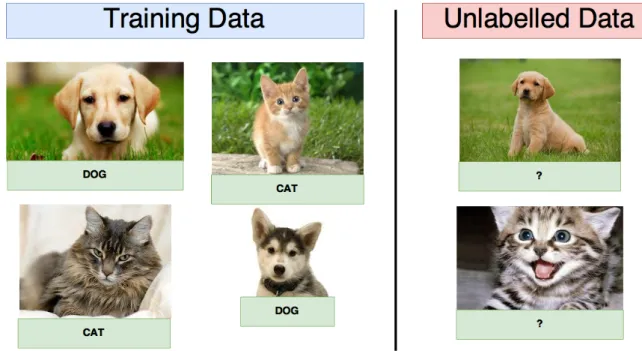
According to their characteristics, problems are divided into different categories on machine learning. This thesis will focus on classification problems, which consists in using an algorithm to predict the classification label of an example of data. To achieve that, the algorithm has to be trained with examples of data and their corresponding labels. In figure 1.1 we can see an example of these problems where the algorithm is fed with characteristics of images, also known as features, and then it is told which ones are cats or dogs, which are the labels of the problem. This is known as the training part and it produces a classifier. Later, new examples of characteristics of images, not used during the train part, are shown to it, and one expects the classifier to be able to classify them. The goal of classification algorithms is to produce a classifier that is
CHAPTER 1. INTRODUCTION 14
Figure 1.1: Example of a classification problem on Machine Learning.
able to accurately predict new data.
Although classification problems have been widely studied, preparing a classifier for such tasks is not easy. It is common for machine learning users to face difficulties such as: how much data is needed, what features should be added, and does the dataset have outliers and/or noisy data [22]. Usually, researchers gather as much information as possible about a problem and turn that into a processed dataset for classification purposes. This methodology often leads to datasets with a large number of features. In these cases, problems such as curse of dimensionality and overfitting are known to deteriorate the performance of the learning algorithm [13, 18, 43]. Therefore, it is critical in any classification problem to reduce the number of features to a smaller subset before training the classifier.
Feature selection (FS) is the process of selecting a subset of the original features so that the feature space is reduced according to a certain evaluation criteria [32]. The goal is to find a smaller subset that yields the minimum generalisation error. This technique can efficiently reduce the dimensionality (number of features) of the problem. Feature selection algorithms are divided into three categories: filter, wrapper, and
embedded [32]. The first ones assesses the quality of features by looking at the
properties of data. Wrappers use the learning algorithm to evaluate subsets of features. Embedded encapsulate feature selection with classifier construction. In addition to these categories, there are hybrid methods which intend to use a filter approach as a
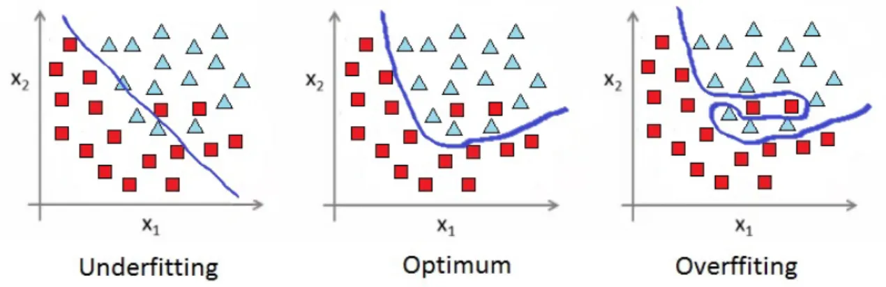
Figure 1.2: Model fitting on training data.
pre-processing step for a wrapper algorithm.
1.1
Motivation
A key requirement to successfully build a classifier is to have data filling the space or at least the part of it where the model is validated [13]. The amount of required data grows exponentially with the number of features (dimensions). Moreover, it is common on classification problems that the chunk of available data is not too large. Therefore, using a high number increases the volume of the space and data becomes sparse through it. This introduces the concept of the Hughes effect [45], which is the name of the curse of dimensionality problem in machine learning. It states that the predictive power of a machine learning algorithm decreases as the dimensionality increases with a fixed number of training examples.
In addition to the Hughes effect, there is other problem that is directly related to using an excessively number of features to produce a classifier. The complexity of a classification model increases with the dimensionality of the dataset. A complex model is more fitted to the training data, which means that it starts ”memorizing” data rather than learn from it. Thus, loosing its capability to generalise and drastically failing to make predictions for new data. This problem is very common and known as overfitting [13, 43]. Figure 1.2 illustrates the three cases for model fitting. On the first one, the model is not fit enough to the data. By contrast, on the last it is overfitted. The image in the middle, represents a model that despite not being able to perfectly predict the training data, will be the best one to predict new examples, which is the goal of the classification problems.
CHAPTER 1. INTRODUCTION 16
High dimension datasets poses a real threat to classification problems. Therefore, feature selection is commonly used as a pre-processing step in these tasks. By lowering the dimensions of datasets, feature selection not only increases the performance of the learning algorithm and the understanding of the classification process, but also reduces computational time of prediction and costs of data acquisition [55]. However, feature selection is a very challenging task. In order to select a subset of features, feature selection algorithms require searching through the feature space, testing subsets of features, and evaluating them to find the final solution. The search space consists of all possible subsets, which for a dataset with n features, produces a search space
of size 2n. This makes finding an optimal subset of features intractable in high
dimensional datasets. Moreover, many problems of this kind are asserted as NP-Hard [38]. Several algorithms exist in literature that tackle this problem. Commonly, they have to compromise the goodness of their solutions in order to provide results in a practicable time.
1.2
Objectives
This thesis presents Mutual Information Two-phased Wrapper Search (MITWS), a new feature selection algorithm based on an hybrid approach. The idea is to first use a filter methodology to reduce the number of features and then apply a wrapper search in order to find the final subset. According to the results reported in literature, wrapper methods tend to find better solutions [30, 17]. However, they are not frequently used in high dimensional datasets due to their computational cost. By using a filter as a pre-processing step before the wrapper search, the feature selection algorithm proposed in this thesis shows that it is possible to use this later technique on datasets with a large number of features.
MITWS will combine an already existing filter approach with a novel wrapper search strategy developed during this work. This new technique, encapsulates a new heuristic that is divided into two phases and intends to propose a different strategy to search for solutions, while maintaining a structure that would favour the use of several processing units. Furthermore, to improve computational performance the novel wrapper will be implemented on both shared and distributed memory parallel environment, using different strategies on each one.
1.3
Thesis Structure
The structure of this thesis is the following. Chapter 2 deals with literature review of feature selection. It starts with a generalization of the problem, explaining each type of algorithm while providing information about the most used ones. Chapter 3 thoroughly explains the MITWS algorithm while chapter 4 discusses the novel wrapper search. Chapter 5 presents two strategies to achieve parallelization of the MITWS algorithm. Chapter 6 address the performance of the implemented work with respect to parallel performance and quality of feature selection. Finally, chapter 7 addresses conclusions and future work.
Chapter 2
Literature Review
The fact that classifiers have low performance for high dimensionality datasets, turns feature selection into an indispensable component on the process of creating them. Given a dataset with several features, the idea of FS is to select those that are relevant, while removing irrelevant and redundant ones (see figure 2.1 for an example). Vergara et al. [58] explain three possible levels of relevance: strongly, weakly, and irrelevant. The first one, refers to features that provide unique information about the class, meaning that they cannot be replaced without loss of information. Weakly relevant features grant class knowledge, still they are not unique in the dataset, and may be replaced by others. Irrelevant features do not contribute with any info, therefore they can be discarded.
In addition to improving classification performance, there are other advantages of feature selection: facilitating data visualization and comprehension, reducing the costs of dataset acquisition and storage, reduce training and classification times [22]. As a consequence, FS has been widely studied. However finding the best features for a classification task is still challenging. The volume of the search space makes it infeasible to perform an exhaustive search in most cases. Therefore, numerous different
Figure 2.1: Performing feature selection on a dataset.
strategies that use heuristics to decrease the computational cost of the problem have been proposed. This led to the existence of several algorithms in the literature. In this chapter, we will discuss the most important ones.
2.1
Classification Problems Workflow
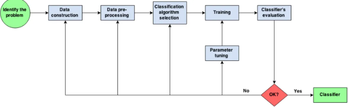
Let us start by analysing the required workflow to solve a classification problem in order to explain the process and to understand where feature selection fits in. The first step for a classification task is to identify the problem. At this stage, the labels for the problem should be defined. The next is to construct a dataset for the classification task. It is crucial that data is related to the problem that is being modelled, otherwise it will not be possible to achieve good classification results. As a simple example, it is not possible to anticipate the weather using heart rate information. In addition to that, only the most informative features about the problem should be used. In cases where there is not a complete knowledge about that, brute-force is an alternative. In this scenario, a large number of variables are measured and inserted into the dataset, expecting that best features can be isolated in the future. As Kotsiantis et al. [31] stated:
”A dataset collected by brute-force is not directly suitable for induction because of the noise and possible missing feature values.”
It is possible to deal with this matter, which leads us to the next step in the clas-sification workflow: data pre-processing. At this stage, key issues such as missing values and outlier detection should be handled. There are several statistic analysis approaches to deal with these problems [1, 26]. Additionally, this is the stage of the problem where the number of features of the problem can be reduced using a feature selection algorithm.
Selecting the classification algorithm is the step that follows. A wide range of classifi-cation algorithms exist, and despite their differences it is not easy to foresee which one is the best for a given problem. Thus, it is a common approach to test and compare several of them, and in the end, keep the one that provides the best results [31]. Classifiers evaluation is most regularly based on the prediction accuracy. A typical technique is to divide labelled data in two thirds to train the model, and use the remaining to test the accuracy. However, this procedure often leads to bad generali-sation outside of the evaluation dataset. Therefore, to reduce the generaligenerali-sation error,
CHAPTER 2. LITERATURE REVIEW 20
Figure 2.2: Workflow for classification problems.
more complex techniques, like cross-validation [29], can be used.
As long as the overall procedure is not able to produce a satisfactory classifier, the process should return to previous stages. There are many causes that may negatively affect the performance of a classifier [31]:
1. Relevant features are not being correctly identified. 2. Dataset does not have enough examples.
3. The number of features is too large.
4. The selected pre-processing technique is not good enough.
5. The elected classifier is not suited for the problem or needs parameter tuning.
Thus, it is not clear to each stage the workflow should return. The ultimate goal of every classification task is to perfectly predict unseen data. However, this is extremely unlikely to occur, and these tasks tend to last very long. Usually, they become an ongoing work where several new attempts are made in order to improve the predicting ability of the classifier. Figure 2.2 illustrates the mentioned workflow.
2.2
General Procedure for Feature Selection
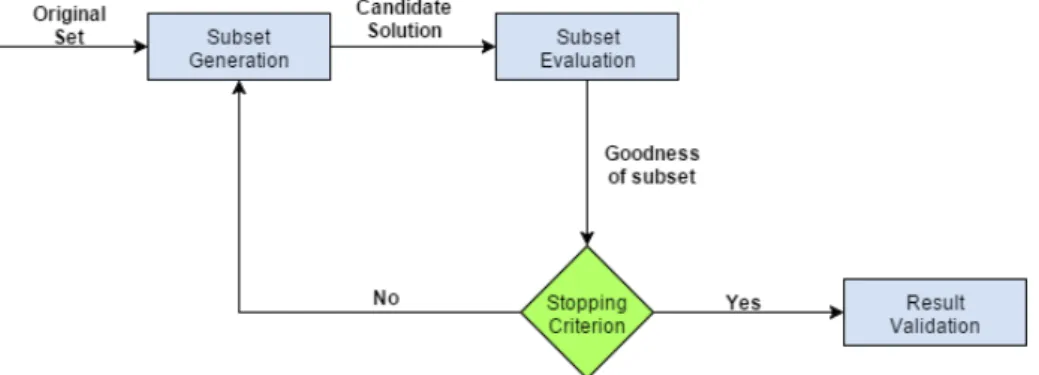
Feature selection algorithms operate by combining a search strategy to find combina-tion of features, with an evaluacombina-tion method to score them. In the end of the process, the highest score subset(s) are considered the solution(s). Despite the existence of sev-eral algorithms, they all follow a gensev-eral procedure that consists of four steps: subset generation, subset evaluation, stopping criteria, and result validation [42, 38, 32].
Figure 2.3: The four steps of feature selection.
The first one determines which subsets will be tested on the process, the next one represents the function that assigns a score to subsets, consequently allowing ranking them. The stopping criteria regulate the intensiveness of the search. Finally, the results validation is the part where the quality of the solution is assessed. Figure 2.3 illustrates these steps, which we will discuss in more detail in the following sections.
2.2.1
Subset Generation
Subset generation represents the process of the heuristic search, where each state in the space specifies a candidate subset for evaluation. Two key issues are addressed at this step: successor generation and search organization.
Successor Generation
Successor generation designates the method for expanding a subset into several new ones. According to authors of [38], there are four basic operators to address this:
• Forward: New subsets are produced by adding multiple features one at the time to the subset to which successors are being generated.
• Backward: New subsets are produced by removing multiple features one at the time from the subset from which successors are being generated.
• Compound: This operator applies k forward steps, followed by l backward ones. By doing so, new iterations between different features are explored [32]. • Random: Subsets are randomly selected.
CHAPTER 2. LITERATURE REVIEW 22
Search Organization
Search strategy designates the walk-path through the states, defining, along the way, from which subsets successors should be generated. This part defines the computa-tional cost of the feature selection algorithm, as well as its ability to find solutions. Therefore, it is plausible to assume this is the most important part of the procedure. Authors of [38] categorized searches into: complete, sequential, and random. Due to the large amount of algorithms that use genetic searches, in this thesis this is added as a category.
• Complete Search: This type of search guarantees finding the optimal solution. The exhaustive approach is an example of a complete search. However, to being characterized as complete, it is not required to be exhaustive. Instead, some heuristic functions may be used to cut the search space, without compromising
optimal solutions. Branch and Bound and Beam Search [53, 21] are some
examples of other complete searches.
• Sequential Search: Define a group of subsets to test in a certain level, and select the best to generate the successors to the next one. From within levels, the number of features on the solutions either increases or decreases one at the time. These searches are easy to implement and usually provide results very fast. However, the quality of the solutions is often poor. Some examples of these searches are stated in [24].
• Random Search: In this approach, the idea is to randomly guide the search. Las Vegas and Las Vegas Incremental algorithms [42] are both examples that fit this category.
• Genetic Search: These are a different type of searches that already incorporate the successor generation. Their idea is to mimic the process of natural selection which consists of three operators: selection, mutation and crossover. Initially several candidate solutions are spawned. Then, the quality of each one is evalu-ated and the best ones are selected. On the next step, new potential solutions are generated combining the elected ones from the previous stage. Genetic operators such as crossover and mutation are used at this point. The process repeats until the end. There are several searches of this type in literature [63].
Due to the importance of this part, it is relevant that the presented searches are further analysed. Sequential ones are the best in terms of computational cost. On a dataset
with n features, most of these methods require testing a maximum of
n
P
i=0
n–i potential solutions. However, they do not produce good results. Their inability to find quality subsets is related to the fact that the addition or removal of a feature to the solution is permanent. During the search, specially in the early stages, there are not any proofs that the elected features should be part of the optimal solution [17]. Therefore, since the beginning the quality is being jeopardized.
The complexity of random searches is totally dependent of the defined amount of tests. Additionally, it is hard to predict the quality of solutions. They rely on the fact that randomness can help escaping from local optima. Usually, these searches are associated to cases where there is an individual ranking of features. Therefore, the randomness of the process can be controlled by it, improving the likelihood of the best features being selected [11].
The computational cost of genetic searches depends on the size of the initial population and on the times the process is repeated. As those numbers increase, so does the probability of finding better solutions. However, these searches tend to converge to local optima [35].
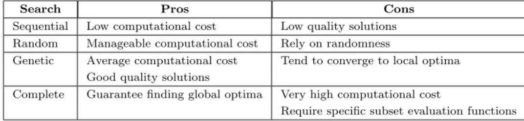
Complete searches find the global optima. However, they have the highest compu-tational cost and tend not to be used in high dimensional datasets [38]. During the process, they rely in a cutting state heuristic. Its intensiveness decreases as more states are cut-off in the early stages. Additionally, these searches, with the exception of the exhaustive one, require using a subset evaluation function that prevents the heuristic from cutting subsets that lead to the global optima. These specific evaluators impact the definition of the optimal solutions conditioning the characteristics of the final solution. The monotonicity property for the Branch and Bound algorithm [53] can be used as an example of these requirements. Table 2.1 summarizes the advantages and disadvantages of the mentioned searches.
Table 2.1: Pros and cons of feature selection searches.
Search Pros Cons
Sequential Low computational cost Low quality solutions Random Manageable computational cost Rely on randomness
Genetic Average computational cost Tend to converge to local optima Good quality solutions
Complete Guarantee finding global optima Very high computational cost
CHAPTER 2. LITERATURE REVIEW 24
2.2.2
Subset Evaluation
This part defines the process of obtaining a score for the subsets tested. The evaluation criterion delineates the quality of a subset and it affects the definition of the optimal solution. More precisely, the global optima to a certain evaluation criterion, may not even be a local optima on a different one. There are two groups that categorize evaluation functions: independent and dependent [38].
Independent Criteria
Independent criteria evaluates the quality of a subset of features considering the characteristics of the data. Most of the times these metrics are used to assess quality of an individual feature. Additionally, they are associated to filter approaches, which will be reviewed in section 2.3.1. Based on the metrics used, these criteria are divided across several categories [42]:
• Distance or divergence measures: the capability of features to differentiate the conditional probability between classes is assessed. Jeffrey’s divergence and Kaga’s divergence are some examples of these metrics [32].
• Information or uncertainty measures: the information that a feature adds to classes is determined. This concept is called information gain, and as an example we have Shannon entropy and all its variants [58].
• Probability of error measures: the ability of a feature to minimize the probability of a classification error is estimated. Bayesian probability is the most known example of this technique [57].
• Dependency measures: assess the capability of features in predicting the labels. Correlation coefficients can be seen as an example [22].
• Interclass distance measures: the distance in the data space is used to determine which are the best features to separate different classes. Euclidian distance is one example of such technique [32].
• Consistency measures: they are based on the principle that features with same values should belong to the same class. The violation of this rule results into a penalty for the feature, allowing a score to be obtained. Some of these approaches are stated in [42].
Dependent Criteria
Dependent criteria use the learning algorithm to estimate the quality of features. Every evaluated subset is used to train the model, then the performance of the later is used to assign a score to the subset. In classifications tasks the most common way to quantify the learning algorithm performance is to use the accuracy of predictions. Evaluation functions that use a dependent criteria are restrictedly associated to wrapper models which will be thoroughly discussed in section 2.3.2.
2.2.3
Stopping Criteria
Stopping criteria defines the conditions to end the search. Some used criteria are [32]:
• The search is complete.
• Some specified bound is reached. The bound may be a defined minimum or max-imum cardinality of the subset of features or a maxmax-imum number of iterations. • Finding a sufficiently good subset.
• The successors of the current state do not improve the evaluation criteria.
2.2.4
Result Validation
After the whole process is completed, a final subset of features is obtained. In order to check whether it is good enough for the problem, it is important to validate it. A straightforward method for validation is to directly measure the solution using the prior knowledge about the dataset. If there is information about the relevant features, it is possible to validate a solution by comparing the selected features against the ones that are known to be relevant. In these cases, information about which features are irrelevant or redundant is also important, mainly because their presence in the solution indicates its quality.
The most common scenario is the lack of knowledge about the dataset. Therefore, different techniques must be used. For example, it is possible to use the performance of the final solution on the model, and compare it to the one obtained with the whole set of features or any other subsets. Additionally, it is normal to use different model algorithms and compare the final solution on them [9].
CHAPTER 2. LITERATURE REVIEW 26
Figure 2.4: Overview of filter approach.
2.3
Categorization of Feature Selection Algorithms
As stated before, there are several feature selection algorithms, which are categorized into three groups: filter, wrapper, and embedded [32].
2.3.1
Filter Algorithms
Filter algorithms use an independent metric to evaluate single features or subsets of features in order to identify which ones are more relevant to the problem. They assume complete independence between the data and the learning algorithm. As result of that, the same strategy can be combined with distinct learning algorithms.
These type of algorithms have low computational cost. However, related to the process of finding solutions, they are known to have worse performance than other types of feature selection algorithms [17].
An overview of filter algorithms is illustrated in figure 2.4. The first state represents the part where the metric is used to obtain a solution. After that, the result is used to train the learning algorithm. In the end, the goodness of the final solution is evaluated at the model evaluation stage.
Section 2.2.2 identified the five types of metrics that can be used in filters. Neverthe-less, filter algorithms can still be divided into univariate or multivariate, depending on the way they search the features [50].
Univariate refers to methods that rank individual features by assigning a score to each one. Then, the rank can be used to select the solution, or to guide a search towards it [15, 6]. These methods are very fast to compute, but fail to remove redundant features that negatively impact learning performance. There are several examples in the literature [6, 16, 22, 60].
On the other hand, feature selection algorithms that evaluate subsets of features are named multivariate. They are known to be extremely efficient in removing redundant features, however they are prone to overfit the model. As a result, it is a common
approach to use a univariate method to filter the most irrelevant features, before using an multivariate method [22]. There exist several algorithms with these characteris-tics [6, 42, 7].
Figure 2.5 illustrates the differences between the two categories.
Figure 2.5: Differences in univariate and multivariate methods.
2.3.2
Wrappers
The idea of wrappers is to use the learning algorithm as a ”black-box” to guide the search towards the solution. Therefore, dependent criteria evaluation functions are used on these models. Figure 2.6 illustrates the overview of a wrapper approach. Since the learning algorithm is used in the process of selecting features, wrappers usually find better solutions [30, 17]. However, these solutions are strictly related to the selected algorithm. Therefore, it is not advisable to use a wrapper to obtain a subset of features with the intention of using it in several learning algorithms.
In terms of computational cost, wrapper algorithms are expensive, since they require training and testing the learning algorithm at least one time for each potential solution. Most of the times, cross-validation techniques are used [17], which even aggravates the problem. As a result, these methods are not frequently used on datasets with large amount of features.
Combining different search strategies with distinct classification algorithms results in creating new wrapper methods. Therefore, there are several algorithms in the
CHAPTER 2. LITERATURE REVIEW 28
Figure 2.6: Overview of wrapper approach.
literature. Some examples are: the hill climbing and best-first search used on Kohavi’s work [30], scatter search [39], sequential backward or forward search [6], and genetic searches [27].
2.3.3
Embedded
Embedded methods are inspired in wrappers and filters, trying to use the best qualities of both. They encapsulate feature nomination with classifier construction. By doing that, the feature selection part interacts with the learning algorithm which results in better solutions, as is the case of wrappers. However, they do not require training the model multiple times, which makes them less computational expensive. Furthermore, these methods are very specific to a learning algorithm. Meaning that an embedded method can only be used with the exact learning algorithm it was built to work with. According to Tang et al. [55] there are three types of embedded algorithms:
1. Pruning: these methods first train the classifier with all the data, and then try to remove features while maintaining the classifier performance. The RFE-SVM algorithm introduced at [23] is an example.
2. Build-in: these approaches have a mechanism that selects the features as it
constructs the classifier. Decision trees are the best known example of this
type [14].
3. Regularization models: these strategies use objective functions to try and minimize fitting errors while eliminating features that are not needed for the learning algorithm. There are several examples of regulation models: L1-norm, LASSO, and Concave Minimization [34, 55].
Figure 2.7 illustrates the overview of embedded algorithms. In the same way as
Figure 2.7: Overview of embedded approach.
the model is being created while features are being selected and it is not ready until the end of the process. Therefore, the model evaluation step has to be done at the end of the whole process.
2.4
Comparing Feature Selection Algorithms
In this chapter many feature selection algorithms were presented, but still many were left out. Performing a comparative study of all of them is a very difficult task. Mainly, because it is very challenging to find out the effectiveness of a FS method, without knowing in advance which features are relevant on the dataset. This is the most common case. Moreover, distinct datasets present different challenges which makes it hard to generalize the quality of algorithms.
The usual way to compare FS algorithms is to use different strategies on the same problem, and assert the quality of each final solution. Parameters such as number of features, accuracy of the model, and time can be used.
Belanche et al. [6], tested several fundamental algorithms to assess their performance in a controlled experimental scenario. Quoted from their conclusion:
”Our results illustrate the pitfall in relying in a single algorithm and sample data set, very specially when there is poor knowledge available about the structure of the solution or the sample data size is limited.”
The mentioned study, reinforces the idea shared by many researchers that there is no clear indication which is the ”best algorithm” for feature selection [41]. Many comparative studies of existing feature selection methods have been done in the literature. For example, the work at [6] applied seven filters, two embedded, and two wrapper methods to 11 synthetic datasets, and compared their performances. Another example is the work of Duch et al. [15], that compared five entropy-based
CHAPTER 2. LITERATURE REVIEW 30
Table 2.2: A taxonomy of feature selection techniques [50].
Model search Advantages Disadvantages Examples
Filter Univariate
Fast Ignores feature dependencies Information Gain
Scalable Ignores interaction with the learning
al-gorithm
Pearson Correlation
Independent of classifier
Multivariate
Models feature dependencies Slower than univariate techniques LVF Independent of classifier Less scalable than univariate techniques FOCUS Better computational complexity than
wrappers
Ignores interaction with the learning al-gorithm
mRMR
Wrapper Deterministic
Simple Risk of overfitting Sequential searches
Interacts with the classifier More prone to getting stuck on local optima
Less computationally intensive than ran-domized
Classifier dependent selection
Randomized
Less prone to local optima Computationally intensive Random searches Interacts with the classifier Classifier dependent selection Genetic searches Models feature dependencies Higher risk to overfitting
Embedded Interacts with the classifier Classifier dependent selection RFE-SVM Better computational complexity than
wrapper
Changing classifier means changing algo-rithm
Decisions trees
Models feature dependencies LASSO
filter methods. Similarly to the first presented study, here authors also concluded that there is not one best method for different datasets. Related to high dimension datasets, work at [14], analysed different FS methods combined with various classifiers. As a conclusion, authors showed the importance of using FS methods instead of all the available features. However, once again they did not conclude that there is a FS method that performs better than all the others. Hao et al. [24] compared the performance of sequential search and genetic algorithms, reaching the conclusion that no algorithm consistently outperforms the others.
Several more studies that compare feature selection algorithms with similar outcomes could be added to the list. Because of that, instead of trying to reason which algorithm performs better, table 2.2 presents the advantages and disadvantages of each type of feature selection.
2.5
Hybrid Approach
The three main categories for feature selection algorithms were discussed. However there is another methodology whose importance has been growing. This relatively new approach is called hybrid and its goal is to combine filter and wrapper methods for
performance improvement. As previously discussed, filter methods are computational fast but often fail to produce good solutions. On the other hand, wrapper methods achieve good results but they are very time consuming, and impracticable to use on high dimensional datasets. The idea behind an hybrid approach is to first use a filter method to reduce the feature space and then adopt a wrapper mechanism to select the final solution. By doing that, a high dimensional dataset will be transformed into a lower dimensional one, therefore using a wrapper approach becomes practical. There are several filter methods that can cut the feature space. For example, the IFSFFS algorithm [60] uses F-score filter metric to rank individual features, then the rank is used to more efficiently guide the wrapper search. On other example, the QBB algorithm [42] applies the LFV filter algorithm in order to generate subsets, which are utilized as starting points for a branch and bound search. One last example is presented in [61], where authors refer to a mutual information metric to remove features before proceeding to a more computational expensive wrapper search.
2.6
Parallel Feature Selection
Selecting the ideal set of features is far from an easy task. It usually requires many attempts until the desired result is attained. A conventional methodology is to change parameters on the algorithms or test different ones to compare results. Moreover, depending on the size of the dataset and on the algorithm chosen, a feature selection process can take a large amount of time.
Parallel computing emerged as a potential solution to tackle this problem. Carrying multiple computations simultaneously to solve a problem relies on the principle that large problems can, in fact, be divided into smaller ones [12]. Taking a closer look into the general procedure for feature selection, it consists in generating and evaluating huge amounts of subsets until a stop condition is reached, and the best subset is provided as final solution. This problem could be easily divided into smaller tasks, where each one is defined as the overall process on each subset, turning feature selection into an ideal candidate for parallel computing techniques. This triggered researchers to exploit parallelism within feature selection algorithms in order to improve their execution times. For example, Azmandian et al. [4] used graphic processing units to accelerate their feature selection algorithm. Lopez et al. [39] also resorted to parallelism to speed up a scatter search in order to obtain better performance in terms of execution time and quality of solution.
Chapter 3
A Hybrid Feature Selection
Approach
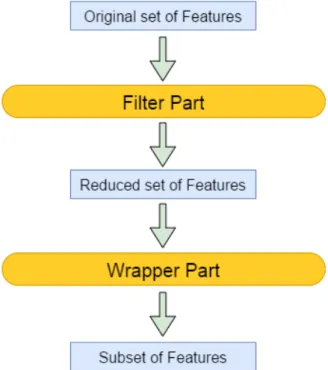
From the previous chapter it is possible to conclude that filter feature selection meth-ods are fast to compute, but often fail to produce good results. Otherwise, wrappers are able to find the best solutions, however the amount of computations required by them are huge, thus making it impracticable to use them on high dimensional datasets. Hybrid approaches emerge as a technique to help in this issue. By using a filter algorithm to decrease the search space of the problem as a first step, they enable wrapper approaches to be used despite the number of features on the dataset.
Inspired by these facts, an hybrid method is proposed in this thesis, combining a filter and wrapper method, aiming to preserve the advantages of both while mitigating their drawbacks. This chapter presents the Mutual Information Two-phased Wrapper Search (MITWS) which is a new hybrid approach and one of the contributions of this work. The innovative algorithm combines an already existing filter approach with a novel wrapper approach developed in the context of this work.
The MITWS algorithm is divided into two parts: filter and wrapper, as illustrated by figure 3.1. The first one, uses an univariate method to rank features individually. Based on a threshold and on the estimated ranks, features are selected to the next phase. The goal of this part is to use a less costly computational method to reduce the search space. Therefore, removed features are considerer irrelevant and are not used any further in the next stages of the algorithm. Individual ranks are obtained using the Mutual Information (MI) [58] as metric to evaluate features. The wrapper part searches the feature space by using a novel meta-heuristic in order to find the final
Figure 3.1: Schematic of the MITWS algorithm.
subset of features. As previously mentioned, wrappers require a learning algorithm to evaluate the goodness of subsets. By comparing Support Vector Machines (SVM) with several learning algorithms in the context of classification problems, Vinodhini and Chandrasekaran [59] show that SVMs in general outperform other classifiers. Thus, making SVMs a more desirable choice for the proposed method.
Two additional algorithms were added to MITWS: Uncertain Class Attribute Inter-dependency Maximization (UCAIM) [19] and Grid Search [37]. The first one is used to discretize data, which is a mandatory procedure to calculate MI in cases where variables have continuous values. The Grid Search is a very popular method used to estimate the parameters of learning algorithms.
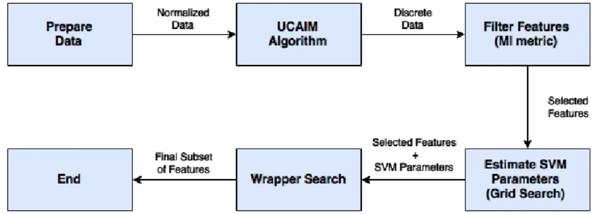
The workflow of the MITWS algorithm is illustrated in figure 3.2. The first step is to prepare data, which will later be discretized with the UCAIM algorithm. Then, the feature space is reduced by eliminating features that are not able to pass the MI filter. The next stage, if necessary, is to estimate the SVM parameters using the Grid Search. Finally, the algorithm executes the wrapper search which is responsible to find the subset of features that is presented as final solution. All the previous steps are explained in more detail in the following sections, with the exception of the wrapper search. Since this last part introduces a novel strategy which makes it the most significant contribution of this thesis, a full chapter is dedicated to it (chapter 4).
CHAPTER 3. A HYBRID FEATURE SELECTION APPROACH 34
Figure 3.2: Workflow of the MITWS algorithm
3.1
Data Preparation
This is the stage where data is read from files and pre-processed. In most cases, this process includes techniques to find outliers that may jeopardize the performance of the learning algorithm. Although there are several techniques to detect and remove them, this process usually requires some knowledge about the dataset. This procedure is rather specific to the data and thus it is not included as part of the present hybrid approach. Instead, MITWS assumes that the dataset is already clean and ready for learning purposes. In any case, this stage implements normalization of the feature values to a scale from 0 to 1. This is a recommended procedure in order to improve the performance of learning algorithms [22].
3.2
UCAIM Algorithm
In order to discretize data, UCAIM, an evolution of the original CAIM algorithm [33] was added to MITWS. Both methods have the goal to delineate intervals on data in such a way that the interdependence between features values and class labels is
maximum. Despite the fact that both algorithms perform well, the evolutionary
approach adds the offset component, which takes into account cases where data is unbalanced (number of examples in the data is not equally distributed by the class labels). The UCAIM algorithm has been shown to outperform the original one in these cases. Moreover, it performs as well as the CAIM on datasets where data is balanced [19].
0 0,1 0,2 0,3 0,4 0,5 0,6 0,7 0,8 0,9 1 U CA IM s tag e Values
Normalized data Possible points Discretization scheme Discrete data
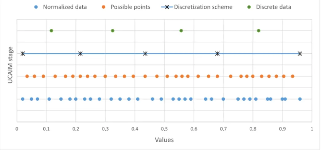
Figure 3.3: Steps of the UCAIM algorithm
of two elements: the maximum and minimum values. Then, it proceeds to define a set of possible points. These are all the midpoints between each adjacent pair in the sorted and non-duplicate set of values. After that, UCAIM iteratively tries to add possible points to D. At each round, all possible points are added, one at the time, to D. Then, formula 3.1, which tries to maximize the interdependence between classes, is used to evaluate the quality of D with the recently added point. At the end of the round, the point with the best score is definitely appended to D. The process stops when no point could improve the score that D has at the start of the round, and there are at least as many intervals as classes. By the end of the UCAIM algorithm, a discretization scheme D is obtained. Later, for each feature value, the interval on D where it belongs is discovered, and the value is converted to the midpoint of that interval. Thus, achieving the desired discrete data.
Algorithm 1 represents the steps required to find D for a given feature Fi and its
possible values Vi on a classification problem with S label classes. Additionally,
figure 3.3 illustrates an example of all the estimated values during different stages of the process. UCAIM(Fi, D) = n P r=1 max2 r×Of f setr M+r n (3.1)
where n is the number of intervals, r iterates through all intervals, maxr is the
maximum value inside an interval, M+r is the total number of values on the interval,
CHAPTER 3. A HYBRID FEATURE SELECTION APPROACH 36 Offsetr = S P i=1 (maxr− qir) S− 1 (3.2)
where S represents the classes labels, qir are the number of values in interval r that
belong to class i, and maxr is the maximum number of values in interval r across all
classes. Basically, Offsetr represents the average difference of the number of points
in all classes to the number of points in the class that has the most points in that interval.
Algorithm 1 UCAIM Algorithm 1: procedure UCAIM(Vi, S)
2: values ← RemoveDuplicates(Vi) 3: min, max ← FindLimits(values)
4: B ← GeneratePossiblePoints(values)
5: K = 1, D ← {min, max},
6: BestS ← 0, BestP ← {}
7: while K ≤ S or GlobalU CAIM < BestS do
8: GlobalU CAIM ← BestS
9: D ← D ∪ BestP
10: for P ∈ B do
11: auxD ← D ∪ P
12: auxS ← GetUCAIMScore(auxD)
13: BestS, BestP ← UpdateBest(P, auxS)
14: K = K + 1
3.3
Filter Part
In contrast to some feature selection algorithms, the aim of the filter part is not to select a final subset of features. Instead, MITWS uses it as a pre-processing step to eliminate features and make it practicable for a more intensive search on the wrapper part. Therefore, the presented filter should have the following characteristics:
1. Evaluate single features. Several filter approaches evaluate subsets of features (multivariate methods section 2.3.1). However, to keep a low computational cost on the presented approach, features are evaluated individually to avoid searching for feature subsets.
2. Not very restrictive. The percentage of removed features should not be
very large. Although as less features pass the filter the faster the wrapper
a metric [32]. Moreover, it has been shown that features considered irrelevant when individually evaluated, are in fact important when inserted into a specific set of features [22]. Hence, to avoid compromising the goodness of the final solution, it is important to avoid removing a large number of features at this stage.
There are several algorithms in the literature that fulfil the first requirement. These
methods are called univariate (section 2.3.1). As previously mentioned, the two
most commonly used univariate metrics are Mutual Information (MI) and Pearson Correlation Coefficients (PCC). Both metrics measure the dependence between two variables. Nonetheless, there is a key difference between them. MI measures the general dependence between the variables while PCC measures linear dependence. Li et al. [36] tested this property and concluded that this makes MI a better metric. Moreover, MI has been widely used on feature selection [58, 22, 15]. For these reasons, MI was selected as metric to evaluate individual features.
In order to calculate MI, a method to estimate the joint probability must be used. To better understand the calculation of MI, suppose that for a feature f , there are i possible values and j possible labels. Hence, Pi,j represents the joint probability of the
ith possible value of f belonging to the label j. Then, to calculate MI the following formula is used: IG(f ) =X i X j Pi,jlog Pi,j (Pi× Pj) (3.3)
Calculating the MI score for every feature does not remove features by itself, so after obtaining the scores, a strategy was defined to create a threshold. The idea is to remove features whose MI score is below the threshold. Since MI scores diverge a lot when changing datasets, a fixed threshold could not be defined. Instead, users are able to manipulate a percentage P which is then used on the formula 3.4 to calculate the threshold. Basically, the threshold is defined as a percentage of the maximum MI score obtained.
threshold = M Imax− (MImax× P ) (3.4)
Although MITWS does not present any restrictions to the definition of the value of P , it is recommended to use a value that does not define a very restrictive threshold.
CHAPTER 3. A HYBRID FEATURE SELECTION APPROACH 38
3.4
Grid Search
SVM was the selected learning algorithm to evaluate subsets of features. These algo-rithms have some parameters that must be tuned in order to provide better results [37]. However, it is common for researchers not to know which parameters should be used because they vary depending on the task. On our proposed method, users are allowed to define the parameters, but if they do not specify them,the algorithm estimates the best to be used.
MITWS tests several parameters and selects the ones that provide the best results using a Grid Search. This method tests parameters in two ranges: first, in a larger one and then, after choosing one value from it, in a smaller scale range. For example, supposing that for a parameter i, the large range is represented by the values Li =
{..., 27, 29, 211, 213, ...} and imagining that the selected value from the L
i is 29, the
algorithm proceeds to search the final parameter value in the following range Si =
{..., 28.5, 28.75, 29, 29.25, 29.5, ...}. There are cases where it is required to estimate more
than one parameter. In these scenarios, all the combinations of possible values and parameters are tested.
To test a possible value for a parameter, a classifier is modelled. Then, the performance of the later is adopted as metric to rank the best values. Typically, Grid Search
is applied on the final classifier in order to tune it. However, on the presented
approach, several classifiers will be handled during the process of selecting the subset of features that will be used on the final one. Moreover, performing a Grid Search for every considered classifier, is not an option. Doing that would increase the wrapper computational cost so much that even with a filter to decrease dataset dimensionality, and parallel computing techniques, it would take huge amounts of time to find a solution for an average number of features. Therefore, the solution is to estimate the parameters before starting the wrapper search.
Our proposed algorithm, performs a Grid Search on n randomly generated subsets before starting the wrapper and after the filter part. The best set of parameters for each subset count as a vote, and in the end, the parameters set with most votes is selected. In cases where the highest number of votes is the same in more than one set, the process generates n new random subsets and the test is reproduced for the tied values. This process is repeated until there are no more ties. Thus, obtaining a final value for the parameters.
on MITWS.
Algorithm 2 Grid Search
1: procedure Grid Search(n, dataset, possibleV alues )
2: subsets ←generateRandomSubsets(n)
3: large = T rue
4: while T rue do
5: votes ← ∅
6: votes ←getVotes(dataset, subsets, possibleV alues)
7: if tiedVotes(votes) then
8: possibleV alues ←filterTiedVotes(possibleV alues, votes)
9: else
10: if large then
11: large = F alse
12: possibleV alues ←getSmallerRangeValues(votes)
13: else
14: break
15: parameters ←getTopVote(votes)
16: 17:
18: procedure getVotes(dataset, subsets, possibleV alues)
19: votes ← ∅
20: for subset ∈ subsets do
21: bestScore = 0
22: bestV alue = 0
23: for value ∈ possibleV alues do
24: score ←getSVMScore(dataset, subset, value)
25: if score > bestScore then
26: bestScore = score
27: bestV alue = value
28: votes ← votes ∪ bestV alue
Chapter 4
Wrapper Search
The proposed feature selection approach was designed to adopt existing algorithms for most of the tasks that must be performed. However, the wrapper search is a new meta-heuristic which, together with the strategies for its parallel execution, makes it the main contribution of this work. It is the most complex part of MITWS and the functions used at this stage define its computational cost and ability to find good solutions. For the sake of understanding, the explanation is further divided into three sections: search strategy, subset evaluation, and successor generation.
4.1
Search Strategy
Despite the fact that several search strategies exist and have been successfully used on wrapper approaches, a novel meta-heuristic which is divided in two phases is introduced in this section. It aims to create a different strategy to search for solutions, while maintaining a structure that can be easily executed with multiple processing units. The proposed search organizes subsets as nodes on a tree, whose first level is composed by n starting subsets, each with a single feature not removed by the filter. Afterwards, subsets are tested and, if they are good candidates, they are further expanded into several more subsets. From now on, the words subsets and nodes are used interchangeably.
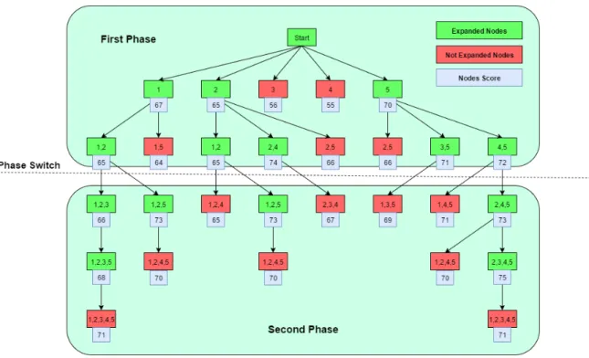
The innovative idea of the proposed search is to explore broadly different regions of the search space, looking for the areas of higher classification accuracy, and then focus on searching the local maxima in each region. Thus, the search strategy does not have
Figure 4.1: Example of the proposed wrapper search.
an uniform behaviour, but is divided into two phases. First, as many good solutions as possible are gathered. Then, they are improved up to the best score they can reach. The transition between phases takes place when subsets reach a certain number of features. Figure 4.1 illustrates an example of the implemented wrapper search. In the first phase, nodes are explored using a breadth first strategy. The decision to expand a node is based on the distance from its score to the global best. In this step, a threshold is defined and nodes whose score differs from the global best by less than a threshold amount, have their successors generated. During the second stage, nodes are explored using a depth first strategy. In addition to that, they are expanded while they still improve the score of the subsets from which they originate. The search stops when there are no more nodes left to explore.
During the second phase in order to avoid excessive work, a mechanism probabilisti-cally cuts subsets based on how distant their score is from the global best, according to the following table:
% Distance to global Cut probability d < 0.5 0% 0.5 ≤ d < 1.0 25% 1.0 ≤ d < 1.5 50%
CHAPTER 4. WRAPPER SEARCH 42
Figure 4.2: How Support Vector Machines work.
The mechanism executes every t seconds, where t is a value which can be user defined. Additionally, the first stage threshold that decides if nodes are expanded and the size at which stages switch, can also be configured. All these parameters have a great impact on the amount of nodes explored in the search. Thus, it is possible to control how restrictive the search is by changing them. Insights about their impact will be given in chapter 6.
4.2
Subset Evaluation
The idea of SVMs is to map vectors of features into higher dimension spaces. Then, finding hyper planes that separate classes, grouping the most points from the same class as possible. Hyper planes are defined using support vectors, which are subgroups of points from each class. Additionally, SVMs have several kernels to choose from. Each one defines a different way to map data into higher dimensions, consequently impacting the position of hyper planes. In order to select an adequate kernel, size and type of data should be taken into account [37]. The number of configurable parameters on SVMs, depends on the adopted kernel. Figure 4.2 illustrates the two crucial components of a SVM. The left one represents the mapping of the data into higher dimensions, and the other, is the hyperplane that divides classes.
The objective of using an SVM component in our strategy is to evaluate the goodness of a subset of features. In order to improve generalisation outside the training dataset, a cross-validation strategy is used at this stage [37]. This technique consists in defining a k number folds and dividing data examples into k groups. Then, for each tested subset, the classifier is trained with k − 1 groups and the accuracy tested with the remaining. This process is repeated k times for each subset. In the end the algorithm
Figure 4.3: Subset evaluation using SVM.
gets a score for the subset. This score is the average of accuracy obtained for each fold. This process is illustrated in figure 4.3.
4.3
Successor Generator
The idea is to expand a subset Sj into several new ones, where each of them is
represented by Sj added with a single new feature that was not part of it. In order
to decide how many successors of a subset are generated, two different options are provided.
The first strategy is to expand a subset Sj into as many successors as the number of
features that are not part of it. For example, if Sj has n features and the total number
of features on the wrapper is K, then expanding Sj will result in K− n new subsets.
One example of this type of expansion is given by figure 4.4a.
An alternative approach, each feature can be added with a specific probability, accord-ing to a likelihood of improvaccord-ing the evaluation score, estimated in a pre-processaccord-ing step described below. By doing so, our approach increases the likelihood of features with high improvement score being added to new subsets. Figure 4.4b illustrates
this process. There, each new subset has a Pi probability of being generated. The
likelihood of a certain feature contributing to an improvement in the evaluation criteria is estimated in a pre-search phase. The procedure starts by generating r random subsets, and evaluates each one of them using the subset evaluation procedure. Then, the improve capability of Fi is assessed by either adding or removing it from each
subset and checking if the score of the subset improved. In the end, the number of times Ii, that a feature improved a subset is obtained and used to calculate the
CHAPTER 4. WRAPPER SEARCH 44
(a) Successor generation without probabilities (b) Successor generation with probabilities
Figure 4.4: The two types of successor generation on the wrapper search
wrapper search decides to expand a node.
Pi =
Ii
r (4.1)
Since the second approach does not expand a subset into all possible successors, it explores a smaller number of nodes. Thus, making the whole wrapper strategy less computational costly. In chapter 6, the impact of both approaches on the final solution and number of subsets tested will be discussed.
4.4
Work Repetition
From the previous section, it was clear that our successor generator function may spawn subsets that have already been tested before. Moreover, from figure 4.1 it is possible to note that the search strategy does not handle the problem. Since the function that evaluates subsets is deterministic, testing a subset more than once is a waste of computations. Additionally, repeated work is a serious issue to the execution time of the wrapper search.
To solve this duplicated work problem, we added an efficient data structure, in this case an hash table. Our strategy consists in producing a unique identifier for every generated subset during the search, and use it as the hash key to save the associated subsets in the hash table. Then, every time the successor generator procedure is
Figure 4.5: Mapping a subset into the hash table
executed, a very efficient table look up checks which of the new spawned subsets have already been generated before. Those that have been generated before are discarded while the new ones have its unique identifier added to the structure.
The hash value is obtained by first sorting the features in a subset, then by adding a comma separator for each pair, and then by converted the whole subset into a string. Finally, any possible hash function can be used to create the entry. The mentioned process is illustrated by figure 4.5.
4.5
Overview of the Wrapper Search
Let us start by explaining the need for a new wrapper strategy and then, introduce the novelty in our strategy. As addressed during the literature review in chapter 2, there is no best method to solve all feature selection problems. This issue is directly related to the fact that a search that guarantees finding the optima solution in a practicable amount of time does not exist. Therefore, proposing new strategies is useful to tackle the problem.
The novelty of the wrapper is related to the developed search. Taking a look at the other components, using a SVM to evaluate subsets of features is a standard procedure that has been used in other cases [62, 40]. Related to the successor generation func-tions, one strategy consists in applying a forward operator introduced in section 2.2.1. The other one uses a similar methodology of feature selection algorithms that ranks features, and then use the rank in order to increase the likelihood of better features being selected. This is the case of the Las Vegas Incremental algorithm [42]. On the other hand, the presented search combines characteristics from different searches in