A Work Project, presented as part of the requirements for the Award of a Master Degree in Finance from the NOVA – School of Business and Economics.
EUR/USD EXCHANGE RATE – CAN IT BE EXPLAINED?
CLÁUDIA GRANJO FERNANDES - 23025
A Project carried out on the Master in Finance Program, under the supervision of:
Professor André Silva
2 EUR/USD EXCHANGE RATE – CAN IT BE EXPLAINED?
Abstract
This paper estimates a present-value model suggested by Engel, Mark and West (2007) applied to the EUR/USD exchange rate for the period from 01/1999 to 12/2015. We present evidence that contrary to what expected, the variable output differential showed a negative impact on the EUR/USD exchange rate. Another interesting finding is the fact that when the sample is restricted to the period of European sovereign-debt crisis, explanatory variables have no longer statistical significance. In addition, in order to validate the performance of the model, we develop a VAR model to analyse the importance of the selected explanatory variables in the model to forecast EUR/USD exchange rate, as suggested by Meese and Rogoff (1982).
3 1. Introduction
Remarkably, foreign exchange rate market is known to be one of the biggest financial markets over the world (King and Rime, 2010). Forecasting exchange rate models have been one of the main concerns of researchers. Empirical international finance points out the failure of traditional exchange rate models in predicting exchange rates. It is a tough task to anticipate fluctuations in exchange rates, mainly for short horizons. Structural and time series models fail due to imprecise parameter estimates errors in fundamentals. Engel, Mark and West (2007) developed a present value model that uses macroeconomic information showing that exchange rates incorporate future information about macroeconomic fundamentals. Meese and Rogoff (1983) together with Cheung et al. (2005) are two interesting papers in which exchange rates were found not to follow a model of exchange rate predictability.
The purpose of this study is to analyse the EUR/USD exchange rate. It will be developed Engel, Mark and West (2007) exchange rate present value model using the macroeconomic fundamentals suggested by the authors and a validation of the forecasting power of that model using Meese and Rogoff (1982) approach. Our aim is to use the simple model by Engel, Mark and West (2007) in order to check its consistency for the EUR/USD exchange rate over 01/1999-12/2015.
Furthermore, we will look to this model and analyse its validity for the period of European sovereign-debt crisis, from 09/2008 to 12/2012. Monthly data will be used as previous studies research demonstrated that the more frequent data is, the better the results estimations and forecast in exchange rate models.
Finally, this study attempts to empirically analyse EUR/USD exchange rate during the mentioned period. Our procedure is based on the mentioned papers. The objective is to understand if during this time span, the EUR/USD exchange rate followed any specific
4 pattern that allow us to make inferences, such as its prediction. For this reason, our study will be based on a present-value model and a VAR model. However, the methodology used might not be exactly the same as in those papers, once here there were made some adjustments in order to be coherent with the data series.
The remainder of this paper is three-fold. We present a briefly analysis the EUR/USD exchange rate from 01/1999 to 12/2015 in section 3. Section 4 contains the present-value exchange rate model that will be used over the study. In Section 5 we describe the exchange rate present value model, including discussion over the period 01/1999-12/2015, while in Section 6 we present the same model but for the period from 09/2008 to 12/2012. Section 7 contains the VAR forecasting model and analysis. Finally, section 8 concludes.
2. Literature Review
Previous literature suggest that exchange rate models have low explanatory power once they have problems with autocorrelation and discontinuities in prices. When taken macroeconomic variables to better explain exchange rates, those never seem statistical significant to determine the movements of exchange rate and when political actions are included in the model, they also have low explanatory power as Ehrmann, Osbat, Strasky and Usukula (2013) stated.
Recently, Engel, Mark and West (2007) suggested a present-value model based on macroeconomic fundamentals. Their results showed that when using macroeconomic fundamentals in exchange rates with a rational expectation model, there is low forecasting power. The authors found these conclusions due to the non-stationarity of macroeconomic fundamentals and also due to the fact that the discount factor of fundamentals in the model was somewhat high (near unit). Meese and Rogoff (1982) analysed the out-of-sample forecast of both structural and time series models. They found that the random walk model achieved
5 better forecasting results for the dollar/pound, dollar/mark, dollar/yen and trade-weighted dollar exchange rates for 12 month horizon.
Also Cheung, Chinn and Garcia-Pascual (2005) set up that exchange rate models mostly cannot outperform the random walk in what concerns to forecasting accuracy. However, according with Mark and Sul (2001) paper, monetary model forecasts that are built on panel estimation methods might have some forecasting power when compared to the random walk, for longer horizons.
Finally, Yesin (2016) studies exchange rate predictability and concluded that models perform better when studying advanced and open economies. The author also stated that attempts to control exchange rate regime did not influenced the forecasting power of the estimations.
3. Exchange rate data
3.1 Stylized facts
Graph 1 represents the nominal EUR/USD daily exchange rate since January 1999 until December 2015, our sample analysis. We can see that there exists volatility clustering. There exist some periods of our data of low volatility and others with high volatility. Another interesting point from this graph is the fact that the tendency line is lowering trough time. Meaning that it has been decreasing over time, however since around 2014 it had an increase.
6 0 0.2 0.4 0.6 0.8 1 1.2 1.4
Daily EUR/USD Exchange Rate
Graph 1 – Daily EUR/USD Exchange Rate
Graph 2 – Monthly EUR/USD Exchange Rate
Graph 2 shows the monthly nominal exchange rate. At first, glance looking at the graph, it seems that the period during the European sovereign-debt crisis appears to have higher volatility. Furthermore, before that period, we can see that the nominal exchange rate decreased until its minimum (0.6258) since the introduction of the euro in Europe.
0.6 0.7 0.8 0.9 1 1.1 1.2 2000 2002 2004 2006 2008 2010 2012 2014 2016 ExchangeRate
7 0 0.0002 0.0004 0.0006 0.0008 0.001 0.0012 2000 2002 2004 2006 2008 2010 2012 2014 2016 Vol_eurous
The impact of European sovereign-debt crisis
After the Great Depression, the financial crisis of 2008-2012 is considered by many researched to be the worst financial crisis. Having its epicentre in the US banking system, many say that the Lehman Brothers collapse was the burst bubble of it. Considering this scenario of collapse of large financial institution, rescue packages which were asked from some countries and prolonged unemployment were some of the results. The fact that some European banks were highly exposed to the US subprime market contributed to an even worst scenario in Europe with this financial crisis. During this period, once exchange rate were even more volatile, risk aversion increased in the investors.
When we look to Graph 3 which represents the monthly volatility of the EUR/USD exchange rate, we observe two big periods of volatility. The last is the European sovereign-debt crisis. The former represents the market’s reaction after the introduction of the euro in Europe.
8 4. Present value exchange rate model
4.1. Theoretical Motivation
Following a Present-Value model for exchange rate from Engel, Mark and West (2007), specifically equation (8) from the mentioned paper, this paper pretends to analyse the EUR/USD exchange rate for the period from 01/1999 to 12/2012 (Model 1) and over the period of European sovereign-debt crisis from 09/2008 to 12/2012 (Model 2). We believe that during these periods and under the following assumptions, this exchange rate model applies for the suggested sample.
Assumptions:
Uncovered Interest Parity (UIP) holds Purchasing Power Utility (PPP) holds No money demand errors
Income elasticity of money demand is unity
Starting with the definition of our dependent variable, and using the asset price intuition for exchange rates, we can state that
𝑠𝑡 = (1 − 𝑏) ∑∞𝑖=0𝑏𝑖𝐸𝑡[𝑓𝑡+𝑖] (1)
Meaning that exchange rate can be represented as the discounted present value of future fundamentals, where s if the log nominal exchange rate, b is the discount factor such that 0<b<1, and f indicated the macroeconomic factors. Thus, this equation implies that exchange rate contains information about future macroeconomic factors.
9 Using Engel, Mark and West (2007), we can set the fundamentals in order to perform this model. Therefore, following the previous stated assumptions, we will rely on a fairly standard but general structure built on the monetary exchange rate model:
𝑠𝑡 = 1 1+𝜆[−(𝑚𝑡 ∗− 𝑚 𝑡) + 𝛾(𝑦𝑡∗− 𝑦𝑡)] + ( 𝜆 1+𝜆) 𝐸𝑡[𝑠𝑡+1] (2)
In which, 𝜆 represents the interest semi-elasticity of money demand, mt the log of the money
supply and yt the log of the output. 𝛾 is the income elasticity of the demand.
This expectation difference equation assumes st as the log of the exchange rate, which is
computed by the log of the domestic currency price of foreign currency as stated in Engel, Mark and West (2007) paper. This formulation means that exchange rate is related to the value of the currency to economic fundamentals. As previous mentioned, for the purpose of this exchange rate model, the economic fundamentals used are the money supply and the output. The money supply is the currency in circulation and the output the Gross Domestic Product. Variables denoted with a * represent foreign variables, in this case, USD variables. Furthermore, and for a matter of simplicity we will assume 𝜆 equal to 10 (the same suggested for the authors of the model).
The no-bubbles forward solution from previous equation is given by:
𝑠𝑡 = 1 1+𝜆∑ ( 𝜆 1+𝜆) 𝑖 ∞ 𝑖=0 𝐸𝑡[−(𝑚𝑡∗− 𝑚𝑡) + 𝛾(𝑦𝑡∗− 𝑦𝑡)] (3)
According with this exchange rate model, two theoretical hypothesis can be made in what concerns to the exchange rate and the future fundamentals previously defined to test in our empirical model:
i. An appreciation of the foreign currency (higher s) implies expectations of lower money growth differential (home versus foreign currency)
10 ii. An appreciation of the foreign currency (higher s) implies expectations of higher
output differential (home versus foreign currency)
4.2 Data
Variables used to perform the following analysis are monthly and cover the period 01/1999 to 12/2012 (Model 1) and the period of European sovereign-debt crisis from 09/2008 to 12/2012 (Model 2). Monthly data was used to reduce the noise of the series and to be easier to identify changes in trends in order to obtain a better strategic long term forecasting.
The variables EUR/USD exchange rate, the output of the US were selected from DataStream while the output variable for Europe was obtained European Central Bank – Statistical Data Warehouse website. The variable money supply was interpreted as the currency in circulation. This variable was selected from the Federal Reserve Data Release for the foreign currency and from European Central Bank – Statistical Data Warehouse website for the European variable. Having all the variables defined, we will now move to the model formulation. In order to understand which fundamentals influence exchange rate, we will move to the formulation of our model.
Preliminary analysis
In a preliminary analysis of the data, we will analyse the variable log exchange rate in Model 1, its distribution and its main statistic indicators. This variable assumes values between -19.75% (minimum) and 6.92% (maximum), with a mean equal to -8.08% approximately. The variable distribution looks like it behaves as a Normal Distribution. When performing the histogram, we quickly analyse the distribution of log exchange rate, and it looks like it could
11 be adjusted to a theoretical shape, which is responsible for the shape of a normal density function, mostly known as Gauss curve given by:
𝑓(𝑥) = 1 √2𝜋𝜎𝑒 −1 2( 𝑥−𝜇 𝜎 ) 2 (4)
In which x represents the log exchange rate, 𝜇 its mean and 𝜎 its standard deviation.
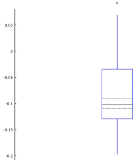
Figure 1 – Distribution of the dependent variable – s.
According with the box plot analysis, in Figure 2, half of the sample had an exchange rate lower than -10.26% (median) and the standard deviation is equal to 6.72%. It is interesting to see that if one could affirm that the percentage distribution of our dependent variable is approximately Normal, then one could also say that the percentage of exchange rate would change approximately between -8.08% ∓ 3 x 6.72%. Therefore, the variance range would be between -28.24% and 12.08%, which corresponds to a variation range of the percentage of the log of exchange rate coherent with reality (-19.75% (minimum) and 6.92% (maximum)).
In this context, a statistical test that allows to analyse with a certain statistical significance if a variable has an approximate Normal distribution will be used.
The Jarque-Bera(JB) test for normality is computed as followed: 0 0.02 0.04 0.06 0.08 0.1 0.12 0.14 0.16 0.18 -0.2 -0.15 -0.1 -0.05 0 0.05 Relative frequency s
12 -0.2 -0.15 -0.1 -0.05 0 0.05 s 𝐽𝐵 =𝑛 6(𝑆 2+(𝐾−3)2 4 ) (5)
Where n is the number of observations, S is the skewness of the sample and K is the kurtosis of the sample. This statistical test lays under the null hypothesis that the data have normal distribution. Meaning that if 𝐽𝐵 > 𝜒2(𝛼,2) 1 then the decision rejects the null hypothesis. This
test is measured by shape indicators about the distribution of the variable (Skewness and Kurtosis). Recalling the previous statistical results, the statistics JB is equal to -13.29. Checking with the Chi Squared distribution, for 2 degrees of freedom and a confidence interval equal to 95%, 5.9912 is the value of which we reject a possibility of believing that the
null hypothesis is true. Well, in this case, as -13.29 is lower than 5.991 we cannot reject the possibility of our dependent variable follow a Normal distribution.
Figure 2 – Box-Plot analysis of our dependent variable – s for Model 1.
1 JB statistics asymptotically has a chi-squared distribution with two degrees of freedom. 2 Usually nominated as the critical value.
13 Summary Statistics
Mean Median Minimum Maximum
Money growth differential 0.15847 0.16039 0.14241 0.16472 Output differential 0.017733 0.011710 -0.028809 0.14229 S – EUR/USD Exchange rate -0.080773 -0.10259 -0.19750 0.069204
Std. Dev. C.V. Skewness Ex. kurtosis
Money growth differential 0.0049452 0.031205 -1.1516 0.55778 Output differential 0.031342 1.7674 1.0629 1.4152 S – EUR/USD Exchange rat 0.067193 0.83188 0.69030 -0.48493
Table 1 – Summary statistics – Model 1
4.3 Methodology
In order to estimate the parameters of the model, the least squares method (MMQ) was used, using EVIEWS statistical software, in order to observe the impact that each of the independent variables would have on exchange rate, maintaining everything else constant. However, in order to test the overall quality of the model and the statistical significance of the parameters in question, we took into account the problems related to the explanatory variables and the randomness of the error. Given the distribution of the error of this random model, it is expected to find a Gaussian distribution. Regarding the explanatory variables, the problem of multicollinearity might arise.
In order to detect the problems described above, it is necessary to use statistical tests, with the exception of the problem of endogeneity. In the case of endogeneity, a graphical analysis can be made between the error and each of the explanatory variables. Note that if we check a pattern between the error and the explanatory variables, it means that the error is dependent on the explanatory variable, otherwise the error is independent. On the other hand, multicollinearity can be detected through the Variance Inflating Factor (VIF2), where its square root indicates how many times the standard error of the parameter associated with it is
14
associated with the variable itself. In this case, if we find a perfect Multicollinearity (R2 = 1),
the MMQ cannot be used because the explanatory variables of the model are perfectly correlated.
However, in order to test the hypothesis that we have a heteroscedasticity problem, we will use a statistical test, White Test. Therefore, to perform statistical tests on the overall validity of the regression model and the statistical significance of the estimated parameters, it is necessary to verify the good behavior of the error and its normality. The overall validity of the model can be evaluated using the F-Snedecor statistical test. Regarding the statistical significance of the model's estimated parameters, it can be determined using the Student-T statistical test. On the other hand, the higher the coefficient of determination, the greater the percentage of the exchange rate explained by the independent variables selected.
With respect to the autocorrelation problem, it can be detected through the Durbin-Watson (DW) statistical test, which is indispensable for making informed decisions regarding the model, assuming the following null hypotheses: H0= no autocorrelation. The significance of this statistical test depends on the number of observations of the sample (n) and the number of explanatory variables of the model (k) that are associated with the critical values of the test, dL and dU, and since it is intended to be in the absence of autocorrelation of the error, the obtained test value must be between 2 and the critical value of dU. Note that the closer the test statistic is closer to 2, the greater the probability that we are in a situation equivalent to the perfect absence of autocorrelation.
15 5. Model 1 - Specification
According to the methodology described above we have estimated the following theoretical model:
OLS model 1
Table 2 – OLS model for the present-value EUR/USD exchange rate model during the period of 01/1999-12/2015.
𝑆 𝑡 = 𝛽0− 𝛽1(𝑚𝑡+𝑗− 𝑚𝑡+𝑗∗ ) − 𝛽2(𝑦𝑡+𝑗− 𝑦𝑡+𝑗∗ ) + 𝜀𝑡 (6) 𝑆 𝑡 = 1.58 − 10.44(𝑚𝑡− 𝑚𝑡∗) − 0.61(𝑦𝑡− 𝑦𝑡∗) + 𝜀𝑡 (7)
The final mathematical model proposed to explain the behavior of the EUR/USD exchange rate between 01/1999 and 12/2015 can explain the reality because the explanatory variables
have statistical significance. In a first analysis of the model we verify that the coefficient of
determination, R2 is 61.93% which means that the explanatory variables can explain around 62% of the variation observed in the EUR/USD exchange rate for the mentioned period.
Coefficient Standard Error T-ratio P-value
Const 1.58376 0.0946012 16.74 5.70e-40
Money growth differential
(𝑚𝑡− 𝑚𝑡∗)
-10.4357 0.595356 -17.53 2.33e-42
Output differential
(𝑦𝑡− 𝑦𝑡∗)
-0.60641 0.093935 -6.456 7.92e-10
Mean dependent var Sum square residuals
-0.080773 0.348892 R-squared F(2.201) Log-likelihood Schwarz criterion rho 0.619330 163.5085 360.3901 -704.8259 0.863463 S.D.dependent var S.E. of regression Adjusted R-squared P-value (F) Akaike criterion 0.067193 0.041663 0.615543 7.00e-43 -714.7802
16 Using the Student-T test to evaluate the validity of the model constant, we find that since its p-value is lower than the critical point, with 95% confidence, we can say that the constant is important for the model. Using the same reasoning for the explanatory variables, we arise at the same conclusion that they are statistical significant for the model.
Therefore, we can make some inferences. Regarding the variable output differential, when related to the EUR/USD exchange rate, the increase of one unit of the first one caused a
decrease in 0.61% of the second one. This result was not expected according with the model.
If we recall the EUR/USD exchange rate present value model stated before, we would expect an increase in the output differential. Nevertheless, the phenomenon observed in the variable of money growth differential (home versus foreign country) was expected, since according to the mathematical model. The increase of one unit of money differential caused a decrease in of 10.44% in the EUR/USD exchange rate.
5.1 Model validity
The analysis of the error behavior is fundamental to accept the final model, since it is necessary to verify the good behavior of the same.
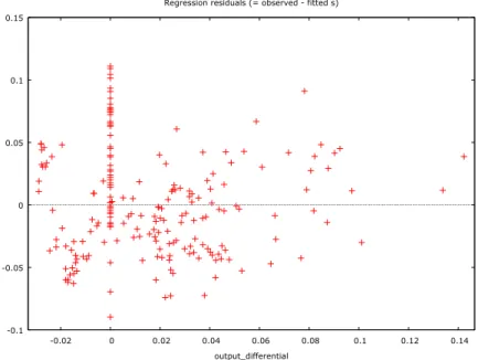
Exogeneity
Using a graphical analysis of the dispersion between the residual and each of the explanatory variables of the model, we observed that the error does not seem to be connected to any of the explanatory variables. A pattern is not evidenced that lead us to believe that we are dealing with a problem of endogeneity that puts into question the randomness of the error and, consequently, the validity of the model. Thus, we might say that we are facing a scenario of exogeneity.
17 -0.1 -0.05 0 0.05 0.1 0.15 -0.02 0 0.02 0.04 0.06 0.08 0.1 0.12 0.14 residual output_differential Regression residuals (= observed - fitted s)
-0.1 -0.05 0 0.05 0.1 0.15 0.145 0.15 0.155 0.16 0.165 residual money_differential Regression residuals (= observed - fitted s)
Figure 3 – Dispersion between the residual of the model and the output differential variable.
Figure 4 – Dispersion between the residual of the model and the money growth differential variable.
Homoscedasticity
In order to analyze the homoscedasticity of the error, in a first approach, we used a graphical analysis of dispersion between the residual model and the explanatory variables. In this sense, when analyzing both explanatory variables, we verified that there seemed to be problems of heteroscedasticity, since it appears that the variance of the error is not constant. However, in
18
order to detect whether or not we are dealing with this problem, we turn to the White Test, assuming the null hypothesis that heteroscedasticity is not present.
Thus, if we were faced with a homoscedasticity scenario with 95% confidence, we would
have to have a nR2 <11.07, since this is the critical value obtained through the Chi-square
table with 5 degrees of freedom. However, since the value of the test statistic is greater than 11.07, we have a heteroscedasticity problem, which leads us to believe that the model error is not random.
Test statistic: TR^2 = 40.162031, with p-value = P(Chi-square (5) > 40.162031) = 0.0000
Normal Distribution
Analyzing graphically the model residue, through a histogram and using the Chi-square test statistic with two degrees of freedom to test the normality of the residual, we have evidence to reject the hypothesis of the error assuming a normal behavior, as observed in figure 4. However, since we have previously verified that it does not have a random behavior, it leads us to conclude that the residue under analysis is not well behaved.
19
Figure 5 – Histogram of the residual of the model.
Autocorrelation
Since we are dealing with a chronological series and not with sectional data, we considered that it was probable that time would help to explain the dependent variable and, if this situation were observed, there could be an error memory and we would have an autocorrelation problem. To detect this situation, we used the DW test statistic. Note that the value obtained corresponding to this test was 0.266625 and, once this value assumed a value lower than 2, we could be in the presence of a positive autocorrelation. In this sense, with a number of observations equal to 204 (n = 204) and the number of explanatory variables equal to 2 (K = 2), we obtain the following table:
dL dU
0 Positive Autocorrelation
1,653 Uncertainty 1,693 2
Table 3 – White’s Test
0 2 4 6 8 10 12 -0.1 -0.05 0 0.05 0.1 Density uhat1 uhat1 N(6.7817e-016,0.041663) Test statistic for normality:
20
It should be noted that the value of the DW statistic is not between the two critical values (zone of uncertainty), being to the left of dL, so we accept the existence of positive autocorrelation in the error, with 95% confidence. To correct the autocorrelation problem, we estimated a new model using the Cochrane-Orcutt estimation. However, as we can see in Table 4, the coefficients of our estimators lost its significance when performing this model. We tried to solve the autocorrelation problem but it was not successful.
Cochrane-Orcutt, using observations 1999:02 – 2015:12 (T=203), rho
Table 4 – Cochrane – Orcutt estimation
5.2 Results and Discussion
We investigate the equation model proposed by Engel, Mark and West (2007) for the EUR/USD exchange rate from 01/1999 until 12/2015. This empirical evidence, based on a
Coefficient Standard Error T-ratio P-value
Const -0.0695577 0.135151 -0.5147 0.6074
Money growth differential
(𝑚𝑡− 𝑚𝑡∗)
-0.133761 0.788654 -0.1696 0.8655
Output differential
(𝑦𝑡− 𝑦𝑡∗)
-0.00891299 0.0282157 -0.3159 0.7524
Mean dependent var Sum square residuals
-0.080989 0.022928 R-squared F(2.200) rho 0.974931 0.062476 0.298385 S.D.dependent var S.E. of regression Adjusted R-squared P-value (F) Durbin Watson 0.067288 0.010707 0.974680 0.939454 1.396992
21
present value exchange rate model links exchange rates to macro variables through expectations. Our results show that nominal exchange rate appears to be well justified by the present value model suggested by Engel, Mark and West (2007) in which some assumptions were made in order to narrow a simple analysis of the topic. However, results should not be totaling reliable, once the error is not random due to detected problems related to Endogeneity and Heteroscedasticity. Nevertheless, these findings are interesting from an economic point of view. Despite the fact the model is not free of error problems, the p-value associated to the explanatory variables are very low. Which suggests that this formulation of the model appears to be suitable when applied to the EUR/USD exchange rate, but results cannot be made with 100% certainty. The results suggest that macroeconomic factors, such as differential output and growth output are related to exchange rates. In addition, the autocorrelation problem and the failure in correcting it, lead us to believe that the estimates of the model parameters are "good" (the estimators are centered), but the error variance is poorly calculated, so the estimators are not efficient, as are the tests T-Student and F-Snedecor are not reliable. In this sense the coefficient of determination may also not be reliable.
6. Model 2 – Specification
OLS model 2
Table 5 – OLS model for the EUR/USD exchange rate during the period of 09/2008 - 12/2012.
Coefficient Standard Error T-ratio P-value
Const 0.456304 0.558546 0.8169 0.4179
Money growth differential
(𝑚𝑡− 𝑚𝑡∗)
-3.56259 3.43095 -1.038 0.3042
Output differential
(𝑦𝑡− 𝑦𝑡∗)
22 𝑆 𝑡 = 0.46 − 3.56(𝑚𝑡− 𝑚𝑡∗) − 0.22(𝑦
𝑡− 𝑦𝑡∗) + 𝜀𝑡 (8)
For the period of European sovereign-debt crisis, the final mathematical model proposed to explain the behavior of the EUR/USD exchange rate is given by equation (8). Comparing to model 1 and therefore, with equation (7), one fact jump insight. With 52 number of observations, none of the explanatory variables have statistical significance in the model. using the Student-T test to evaluate the validity of the model explanatory variables, we find that since its p-value is higher than the critical point, with 95% confidence, we can say that they do not seem to be significant in the model.
6.3 Results and Discussion
One interesting conclusion about this model is the fact that, when we restrict our analysis for the period of European sovereign-debt crisis, from 09/2008 to 12/2012, explanatory variables do not have statistical significance. This results lead us to believe that this is not precise for
periods of crisis. The addition of other variables such as monetary authority’s policies and
public debate by policy makers, suggested in Ehrmann, Osbat, Starsky and Uuskula (2013), might contribute to a better explanation of EUR/USD exchange rate during the period of European sovereign-debt crisis.
7. VAR forecasting analysis
In 1982, Meese and Rogoff suggested an approach to study the validity of exchange rate models and its forecast power. Instead of forecasting the fundamental values from the exchange rate model, this approach consists of comparing out-of-sample forecast to the random walk. The advantage of using this methodology from Meese and Rogoff (1982) is the
23 fact that the vector auto-regressor (VAR) model allows that explanatory variables to be endogenous. In fact, the variable money supply, which is typically used as exogenous variable in the underlying theoretical model used before, could be more realistic if used as endogenous variable. This is supported by VAR results in Meese and Rogoff (1982).
For the purpose of this study, we examine a VAR model with the two explanatory variables used before for present-value exchange rate model in order to analyse how these variables influence exchange rate model forecasts.
The VAR model is the following:
𝑠𝑡 = 𝛼1,1𝑠𝑡−1+ 𝛼1,2(𝑚 − 𝑚∗)𝑡−1+ 𝛼1,3(𝑦 − 𝑦∗)𝑡−1+ 𝛼1,4+ 𝜀𝑡 (9)
(𝑚 − 𝑚∗)
𝑡= 𝛼2,1𝑠𝑡−1+ 𝛼2,2(𝑚 − 𝑚∗)𝑡−1+ 𝛼2,3(𝑦 − 𝑦∗)𝑡−1+ 𝛼2,4+ 𝜀𝑡 (10)
(𝑦 − 𝑦∗)
𝑡 = 𝛼3,1𝑠𝑡−1+ 𝛼3,2(𝑚 − 𝑚∗)𝑡−1+ 𝛼3,3(𝑦 − 𝑦∗)𝑡−1+ 𝛼3,4+ 𝜀𝑡 (11)
According with the authors, the fact that each equation is estimated by OLS is an “efficient estimation strategy”.
7.1 Methodology
We estimate a VAR model for monthly data from 01/1999 to 12/2015. Firstly, we will perform the Augmented Dickley-Fuller test in order to test the stationarity of our variables, to verify if variables are invariance under time shift. Variables found not stationary, the first difference was made. Secondly, in order to check for serial correlation, we perform a LM test for residual autocorrelation, in which the null hypothesis represents no serial correlation in the residuals. Thirdly, we check the normality of residuals. Therefore, we perform the JB test.
24 In order to determine the optimal lag length of the VAR, we use the methodology of lag-order selection, selected by Schwarz's Bayesian information criterion (SC)3. Regarding the stability conditions of the model, we analyse the roots of the system inside the unit circle.
In order to evaluate model performance, MAE and RMSE were applied. The robustness of this metrics has been studied before, but still there is no consensus about the best one to use. For example, Willmott and Matsuura (2005) highlighted some worries about RMSE metric. However, the suggestion of using MAE instead of RMSE is not the key. In theory, RMSE is a better approach for cases when the error distribution of the model is estimated to be normal (Gaussian). In addition, MAE represents the dispersion in error results between the forecasted and the actual value. The downside of this metric is the fact that the relative error’s dimension usually is not that obvious.
Knowing that both approaches have their limitations, we believe that a combination of both metrics is appropriate for the analysis of the model performance. For the purposes of this study, we will compare RMSE and MAE metrics to control for large but uncommon errors in the forecast output. In case there is a big spread among these two methods then it indicates that the error might not be consistent.
The used metrics are calculated as following:
𝑀𝐴𝐸 =1 𝑛∑ |𝑒𝑖| 𝑛 𝑖=1 (12) 𝑅𝑀𝑆𝐸 = √1 𝑛∑ |𝑒𝑖 2| 𝑛 𝑖=1 (13)
Random Walk process
The random walk is inserted in the non-stationary process, that is, all the characteristics of the behavior of the process are not changed in time, that is, the process develops in time around the mean.
25 The reason why we compare VAR to the random walk is because exchange rate series is theoretically followed by a random walk. Therefore, our aim is to analyse whether the model is able to outperform the random walk or not.
7.2 Model validity
Primarily, we must check whether our VAR model has satisfied all the assumptions or not. It was done the first difference of both series s (logarithm of exchange rate) and (m-m*) the money growth differential in order to make them stationary. As previous stated, lag selection is made under the SC information criterion, and so we end up to a VAR (1,2) model. In addition, it is important to stress the fact that the choice of the optimal lag also took into consideration the correlation between time t and t-1 of the model.
Therefore, in what concerns to serial correlation, once the probability of LM-Statistic is higher than our critical point, so accept the null hypothesis meaning that there is no serial correlation in our VAR model. Regarding the statibility condition we can say that no root lies outside the unit circle, meaning that the VAR model satisfies the stability condition.
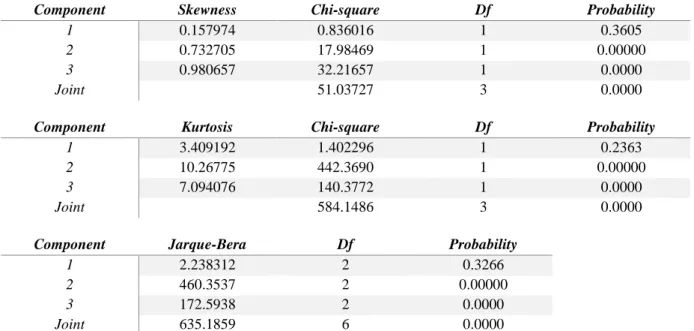
Lastly, in order to check the normality of residuals we perform the JB test under the null hypothesis of residuals are normally distributed, and we verify that under the Cholesky of covariance (Lutkepohl) orthogonalization method, variable EUR/USD (s) is normally distributed, which is desirable. For the model of money growth differential and output differential, we reject the null hypothesis that residuals are not normally distributed. Once the model passes the diagnostic test, we can go through the forecast.
The following equations represent the final mathematical VAR (1,2) proposed model.
26 (𝑚 − 𝑚∗) 𝑡= −0.3881𝑠𝑡−1− 0.0404(𝑚 − 𝑚∗)𝑡−1− 2.6509(𝑦 − 𝑦∗)𝑡−1− 3.9𝐸 − 05 + 𝜀𝑡 (13) (𝑦 − 𝑦∗) 𝑡 = −0.0339𝑠𝑡−1+ 0.0018(𝑚 − 𝑚∗)𝑡−1+ 0.3679(𝑦 − 𝑦∗)𝑡−1+ 0.0047 + 𝜀𝑡 (14) Stability condition Root Modulus 0.836499 0.836499 -0.442881 0.442881 0.168248-0.322979i 0.364175 0.162846+0.322979i 0.364175 -0.190617-0.134192i 0.233115 Table 6 – VAR stability condition
Normality tests
Component Skewness Chi-square Df Probability
1 0.157974 0.836016 1 0.3605
2 0.732705 17.98469 1 0.00000
3 0.980657 32.21657 1 0.0000
Joint 51.03727 3 0.0000
Component Kurtosis Chi-square Df Probability
1 3.409192 1.402296 1 0.2363
2 10.26775 442.3690 1 0.00000
3 7.094076 140.3772 1 0.0000
Joint 584.1486 3 0.0000
Component Jarque-Bera Df Probability
1 2.238312 2 0.3266
2 460.3537 2 0.00000
3 172.5938 2 0.0000
Joint 635.1859 6 0.0000
27 7.3 Results and discussion
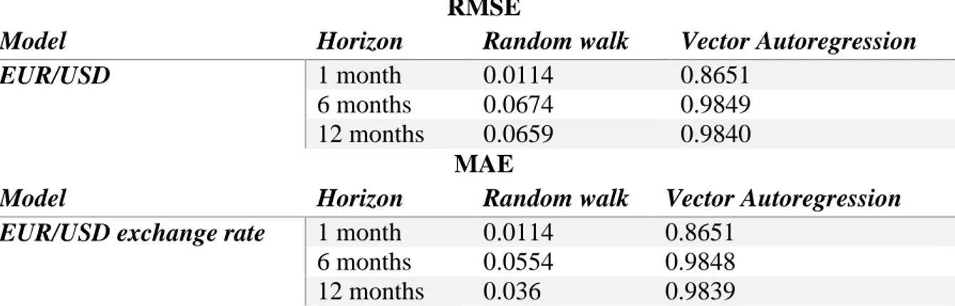
Following Meese and Rogoff (1982) paper, this study analyses the out-of-sample forecasting power of the time series model of EUR/USD exchange rate suggested before. For this purpose, we present in Table 8 regarding the Root Mean Square Error (RMSE) and Mean Absolute Error (MAE) for a VAR(1,2) model and a random walk without drift. We tested the forecasting power for 1 month, 6 months and 12 months. It is possible to realize from Table 8 that the RMSE is close to 1 for the three different horizons for the VAR model. For the random walk model, it was obtained the lowest RMSE for one month horizon.
RMSE and MAE analysis
RMSE
Model Horizon Random walk Vector Autoregression
EUR/USD 1 month 0.0114 0.8651
6 months 0.0674 0.9849
12 months 0.0659 0.9840
MAE
Model Horizon Random walk Vector Autoregression EUR/USD exchange rate 1 month 0.0114 0.8651
6 months 0.0554 0.9848
12 months 0.036 0.9839
Table 8 – RMSE and MAE for the VAR (1,2) model and for the Random walk model.
Another useful tool to analyse the out-of-sample forecasting porwer is the MAE. When looking to the corresponding output of MAE for both Random walk process and Vector Autoregression model, we verify that the one month horizon is again the lowest for the Random walk. However, this time we see that a horizon of 12 months seems to have better forecasting power than 6 months horizon. In what concerns to the Vector Autoregression, once again values are close to 1, meaning that there exists a spread in the values and therefore it has very low forecasting explanation power.
28 8. Conclusions
In this paper, we use the present-value exchange rate model proposed by Engel, Mark and West (2007) in order to determine the contribution of macroeconomic fundamentals to exchange rate movements. We show that when applying observed macroeconomic fundamentals, such as money growth differential and output differential are related to exchange rates, however, results cannot be made with 100% certainty due to some econometric problems such as Endogeneity Heteroscedasticity and Autocorrelation.
When applying the model for the period of European sovereign-debt crisis, macroeconomic factors that showed to be statistical significant for the full sample, found not to be during this period. One explanation for these findings might be related with the fact that exchange rates have clustering volatility and especially during crisis period, they are even more volatile. The European debt-sovereign crisis is particularly interesting from investor’s point of view. During this period, many factors played a role, namely political actions and market news.
However these factors are difficult to measure, including monetary authority’s policies and
public debate by policy makers variables might contribute to a better explanation of the movements of EUR/USD exchange rate during this period (see Ehrmann, Osbat, Starsky and Uuskula (2013)).
The second part of our study we presented a VAR (1,2) model together with the random walk in order to analyse the forecasting ability of the model. What was found was that the suggested time series model could not outperform the random walk model at any studied horizon. This finding goes along with what Meese and Rogoff (1982) stated about out-of-sample forecasting performance.
The advantage of using this methodology from Meese and Rogoff (1982) is the fact that the vector auto-regressor (VAR) model allows that explanatory variables to be endogenous. In
29 fact, the variable money supply, which is typically used as exogenous variable in the underlying theoretical model used before, could be more realistic if used as endogenous variable.
In addition, the fact that it was used monthly data to perform the analysis might have helped to the achieved results. For further analysis, it would be interesting to analyse whether the implemented model applies for periods of low volatility. During this study we found that the present value model did not work for the European sovereign-debt crisis. Meaning that for periods of high volatility, this specifically model is not robust enough to explain exchange rate movements. Looking back to EUR/USD exchange rate time series since 1999 we realize that until 2015 there existed two periods of high volatility. During 200-2002, period at which EU Member States adapted its economy to the new currency of all, and 2008-2012 the European sovereign-debt crisis. What we found here was that indeed a random walk model do better than existing macroeconomic models for the EUR/USD exchange rate.
Finally, in order to increase the capability of the performed test and once classic VAR model can experience over-parameterization, a Bayesian estimation approach by Litterman (1979) could be an efficient way to decrease the RMSE when forecasting up to three years horizon.
30 Bibliography
Campbell, J. A. (1997). The Econometrics of Financial Markets. New Jersey: Princeton University Press.
Charles Engel, N. C. (2007, August). EXCHANGE RATE MODELS ARE NOT AS BAD AS YOU THINK. pp. 5-10.
Cheung, C. a.-P. (2005, JULY). EMPIRICAL EXCHANGE RATE MODELS OF THE NINETIES: ARE ANY FIT TO SURVIVE?
Hamilton, J. (1994). Time Series Analysis. Princeton : Princeton University Press.
Lucio Sarno, M. S. (2013). WHICH FUNDAMENTALS DRIVE EXCHANGE RATES? A CROSS-SECTIONAL PERSPECTIVE. pp. 4-6.
Michael Ehrmann, C. O. (2013, APRIL). THE EURO EXCHANGE RATE DURING THE EUROPEAN SOVEREIGN DEBT CRISIS. DANCING TO ITS OWN TUNE?, pp. 8, 9, 12, 13.
Mills, T. (1999). The Econometric Modeling of Financial Time Series , Second Edition. Cambridge : Cambridge University Press.
Richard A. Meese, K. R. (1982). EMPIRICAL EXCHANGE RATE MODELS OF THE SEVENTIES Do they fit out of sample? pp. 4-8.
Rossi, B. (2005). Are Exchange Rates Relly Random Walks? Some Evidence Robust to Parameter Instability. 6-9.