Os artigos dos Textos para Discussão da Escola de Economia de São Paulo da Fundação Getulio Vargas são de inteira responsabilidade dos autores e não refletem necessariamente a opinião da
FGV-EESP. É permitida a reprodução total ou parcial dos artigos, desde que creditada a fonte. Escola de Economia de São Paulo da Fundação Getulio Vargas FGV-EESP
Janeiro de 2017
Working
Paper
438
Reinterpreting the Mutual Fund Theorem:
The Risk Portfolio as a Tactical Overlay
Os artigos dos Textos para Discussão da Escola de Economia de São Paulo da Fundação Getulio Vargas são de inteira responsabilidade dos autores e não refletem necessariamente a opinião da
FGV-EESP. É permitida a reprodução total ou parcial dos artigos, desde que creditada a fonte. Escola de Economia de São Paulo da Fundação Getulio Vargas FGV-EESP
Reinterpreting the Mutual Fund Theorem:
The Risk Portfolio as a Tactical OverlayPaulo Tenani
São Paulo School of Economics, FGV January 6th 2017
Abstract
The Mutual Fund Theorem is an elegant way of describing how investors with different attitudes towards risk should construct their portfolios. It is, however, often misinterpreted. This paper revisits the topic by defining the Risk Portfolio as a self-financed tactical overlay portfolio in which all the overweight and underweight positions cancel each other out. In this sense no net resources are ever allocated to the Risk Portfolio and all the investment is allocated to the Minimum Variance Portfolio. Under these circumstances the Mutual Fund Theorem implies that the ratio of Bonds to Stocks in the Total Portfolio would depend on investor´s risk aversion; as it is actually observed in practice. The paper also argues that the Asset Allocation puzzle, as traditionally stated in the literature, only arises because of a misconception about the “the facto” definition of the Risk Portfolio.
Key Words: Mutual Fund Theorem, Asset Allocation Puzzle, Modern Portfolio Theory, Minimum Variance Portfolio, Risk Portfolio.
I
I
.
.
I
I
n
n
t
t
r
r
o
o
d
d
u
u
c
c
t
t
i
i
o
o
n
n
The Mutual Fund Theorem is a simple and elegant way to describe how investors with different attitudes towards risk should construct their portfolios. It is traditionally stated as saying that every investment decision consists of three steps. First, there is the construction of the Minimum Variance Portfolio; secondly, the construction of the Risk Portfolio; and thirdly and last, the Asset Allocation Decision on how much to allocate between the Minimum Variance and the Risk Portfolio - a decision that will depend on each investor´s risk-aversion. The objective of this paper is to argue for a different interpretation of the Mutual Fund Theorem; one in which there is no Asset Allocation between the Minimum Variance and the Risk Portfolio. This would happen if the Risk Portfolio were interpreted as, using Asset Management jargon, a “tactical overlay”; composed of only underweights and over-weights allocations that sum up to zero. In other words, the Risk Portfolio would be completely self-financed requiring no net resources whatsoever to be invested in it. All investments, in fact, would be allocated to the Minimum Variance Portfolio and changes in risk-aversion would exclusively result in changes in the magnitudes of the over and under-weights positions within the Risk Portfolio.
It is important to mention that such an interpretation of the Mutual Fund Theorem arises naturally whenever the first order conditions for the investor´s maximization problem are written in a slightly different manner than what is usually done in the traditional Finance literature1; allowing for the coefficient matrix to be inverted even in the presence of a Riskless Security. The solution that arises from this procedure is a clear illustration of how all assets in
1 For example Ingersoll (1992), Elton, Gruber and Brown (2009), Pennacchi (2008) as well as Merton
the Portfolio contribute to both the Minimum Variance as well as the Risk Portfolios; with the Riskless security, when it exists, being also part of the Risk Portfolio.
The intuition, however, is much less clear if one writes the first-order conditions in the traditional manner; in which the Variance-Covariance Matrix of the Portfolio is also the coefficient matrix. Under these circumstances, in the presence of a Riskless Security, the coefficient matrix cannot be inverted, which has led traditional Finance textbooks to arbitrarily exclude the Riskless Security of the Total Portfolio and then solve an Asset Allocation Problem between the Riskless Security and the newly defined Risk Portfolio. It is exactly this procedure that has led the Mutual Fund Theorem to be misinterpreted in the Finance literature, as illustrated by the Asset Allocation Puzzle described in Canner, Mankiw and Weil (2001).
What happens is the following. According to the Mutual Fund Theorem, all assets within the Risk Portfolio should have the same proportions to each other, independently of the investor´s risk aversion. However, in practice, less/higher risk-averse investors tend to have a different share of Bonds over Stocks in their Total Portfolios. Is this an Asset Allocation Puzzle or just a misinterpretation of the Mutual Fund Theorem? It is, in fact, a misinterpretation. And it is a misinterpretation because one is simply confusing the Risk Portfolio with the Bonds and Stocks portion of the Total Portfolio; which, as we will see below, is just not the Risk Portfolio as implied by the Mutual Fund Theorem. This typical and erroneous interpretation of the Risk Portfolio would be innocuous - in terms of the Asset Allocation Puzzle - if there existed a Riskless Security. However, in the absence of a Riskless Security, Bonds and Stocks, as well as the others risk securities, would all be part of the Minimum Variance as well as the Risk Portfolios. So, while by the Mutual Fund Theorem one should expect the share of Bonds over Stocks to be the same in the Risk Portfolio of all
investors; this should not be the case in their total Portfolios. In fact, using historical data, the Mutual Fund Theorem indicates that less risk-averse investors should hold a higher proportion of Bonds over Stocks in their total Total Portfolios.
The paper is organized as follows. Section II describes the investor´s problem in a mean-variance framework and then derives the first order conditions for an optimal allocation. To allow for the coefficient matrix to be inverted even in the presence of a Riskless Security, the first order conditions for the investor´s problem are written in a slightly different manner than in Merton (1972), keeping the Lagrange multipliers on the left-hand side of the equations while moving the Expected Return terms to the right-hand side. This will result in a bordered coefficient matrix that can be inverted even in the presence of a Riskless security. Section III illustrates the traditional manner in which the first order conditions are usually represented in the Finance literature, with the Variance-Covariance Matrix also being the Coefficient Matrix. Section IV then states and proves nine properties of Mean-Variance Efficient Allocations as well as Mean-Variance Efficient Portfolios. But, most importantly, Section IV defines the Minimum Variance Allocations and the Minimum Variance Portfolio as being the equivalents, in Asset Management jargon, to the Strategic Allocation and the Strategic Portfolio – where the totality of the investment is allocated - while the Risk Allocations and the Risk Portfolio would be the equivalents to the Tactical Allocation and Tactical Overlay Portfolio – which is completely self-financed. This is a result that is not sufficiently emphasized in the Finance literature but that this paper intends to stress. Section V illustrates, with numerical examples, the main results of Section IV as well as one solution to the Asset Allocation Puzzle proposed by Canner, Mankiw and Weil (1997). Section VI finally concludes.
I
I
I
I
.
.
T
T
h
h
e
e
I
I
n
n
v
v
e
e
s
s
t
t
o
o
r
r
´
´
s
s
P
P
r
r
o
o
b
b
l
l
e
e
m
m
Consider a portfolio P consisting of N securities with the expected return on the ith security denoted by ri; the covariance between the returns on the ith and jth securities denoted
by σij, and the variance of the ith security denoted by σii = σi2. Let ai be the percentage value of
portfolio P that is invested in security i. Under these definitions, the return and variance of portfolio P are given by the following expressions:
1)
N i i i p ar R 1 2)
N i N i N i j j ij j i i i p a a a 1 1 1 2 2 2 The utility of the investor,U
E
Rp;2p
, is defined over the expected return, E[Rp] , and the variance of the portfolio, 2p, - with the first and second order derivatives having the usual signs: U1´ > 0; U2´ < 0; U11´´ < 0; U22´´ > 0. The investor´s problem, is to find a vector of security allocations ai; i = 1,……..,N, that maximizes utility subject to the constraint that thesum of these allocations is equal to the leverage of the portfolio k.
3)
N i i k a 1Defining as the Lagrange multiplier, the Lagrangian for this problem is given by:
N i i p p i U E R k a a 1 2 ; ; The first order conditions are a system of N+1 equations comprised of equation 3) as well as the following system of N linear equations:
4)
i N i j i j ij j i i E R U U U a a ) 2 ( ) 2 ( 2´ ´ 1 ´ 2 2
i = 1,...N.Notice that the system of N equations in 4) is written with the modified Lagrange multiplier as a right-had side variable; which allows one to write the system of N + 1 first order conditions in matrix form as follows:
k r E U U r E U U r E U U r E U U r E U U U a a a a a N N N N N N N N N N N N N N N N N N N N N N N ) 2 ( ) 2 ( 3 ) 2 ( ) 2 ( ) 2 ( ) 2 ( * 0 1 1 1 1 1 1 1 1 1 1 ' 2 ' 1 1 ' 2 ' 1 ' 2 ' 1 2 ' 2 ' 1 1 ' 2 ' 1 ´ 2 1 3 2 1 2 1 , 3 , 2 , 1 , , 1 2 1 3 , 1 2 , 1 , 1 , 3 1 , 3 2 3 2 , 3 1 , 3 , 2 1 , 2 3 , 2 2 2 1 , 2 , 1 1 , 1 3 , 1 2 , 1 2 1 Or, using matrix notation, 5) Q . A = R
Matrix Q is a (N+1; N+1) coefficient matrix composed by the (N ; N) variance-covariance matrix bordered by the coefficients of the linear constraint in equation 3) as well as the marginal-utility-adjusted Lagrange multiplier. Notice that, because of the border, matrix Q can still be inverted even in the presence of a Riskless Security - a security with zero variance and covariance terms. Vector A is a (N+1 ; 1) parameter vector with the elements of the first N rows being the allocation in the N securities of the portfolio, ai , and the
marginal-utility-adjusted Lagrange multiplier (/(-2U2´ )) as the element at the N+1 row. Vector R is a
(N+1 ; 1) right-hand-side vector composed by the N marginal-utility-adjusted expected returns of the securities in the portfolio; (U1´/(-2U2´)).E[ri] , i = 1, ….., N, as its first N
From this point on we will be calling the term
( 2 2')
'
1 U
U the return-risk preference parameter. Notice that a lower/higher
U1' (2U2')
indicates either a higher/lower marginal utility with respect to the variance term or a lower/higher marginal utility with respect to the Expected Return term and thus, a more/less risk-averse investor.Adding to the above notation, define four additional (N+1 ; 1) vectors, that will be used in the sections below: vectors Z, Z’, R’, R’’. Vector Z is composed of N zeros as its i = 1…....N elements and the degree of leverage k as its N+1th element. Vector Z’, on the other
hand, is composed of N zeros as its i = 1…....N elements and a 1 (one) as its N + 1th element. Vector R’, is composed of the N marginal-utility-adjusted expected return terms,
U ( 2U )
.E
ri' 2 '
1 ) as its i = 1, …., N elements, and a zero as its N+1
th element. Similarly,
vector R’’, is composed of the N expected returns, E
ri as its i = 1, ….,N elements, and a zero as its N+1th element.Finally, the minors (i , j) of matrix Q will be called Qi,jand, whenever the elements of a certain vector V, for V = R, R’,Z, Z’ , are substituted in column i of matrix Q, the resulting matrix will be called QiV.
I
I
I
I
I
I
.
.
T
T
h
h
e
e
I
I
n
n
v
v
e
e
s
s
t
t
o
o
r
r
´
´
s
s
P
P
r
r
o
o
b
b
l
l
e
e
m
m
a
a
s
s
t
t
y
y
p
p
i
i
c
c
a
a
l
l
l
l
y
y
s
s
t
t
a
a
t
t
e
e
d
d
i
i
n
n
t
t
h
h
e
e
F
F
i
i
n
n
a
a
n
n
c
c
e
e
l
l
i
i
t
t
e
e
r
r
a
a
t
t
u
u
r
r
e
e
It is interesting to compare the system of N + 1 first-order conditions as described in equation 4), with the way it is typically described in Finance textbooks. This is represented below:
4’)
i N i j i j ij j i i E R U U U a a ) 2 ( ) 2 ( 2´ ´ 1 ´ 2 2
i = 1,...N. 3)
N i i k a 1Or, in Matrix form
1 ' 2 ' 1 ´ 2 1 ' 2 ' 1 ´ 2 1 ' 2 ' 1 ´ 2 1 ' 2 ' 1 ´ 2 1 ' 2 ' 1 ´ 2 5 4 3 21 1 2 1 3 2 1 1 2 1 13 12 11 3 1 3 2 3 32 31 2 1 2 23 2 2 21 1 1 1 13 12 2 1 ) 2 ( ) 2 ( ) 2 ( ) 2 ( ) 2 ( ) 2 ( ) 2 ( ) 2 ( ) 2 ( ) 2 ( * r E U U U r E U U U r E U U U r E U U U r E U U U a a a a a N NN N N N N N N N N N N N N N N N 3)
N i i k a 1That is, in the traditional Finance textbooks, the first order system of equations is organized so as to solve for the optimal allocations a , i = 1, 2, ...,N in terms of the Lagrange i multiplier. Then, summing up all a , one can use 3) to solve for the Lagrange multiplier i which is substituted back in the expressions for a , i = 1, 2, ...,N to get the final results. i
Notice, however, that by describing the first-order conditions as above, the Variance-Covariance Matrix of the Portfolio is also the coefficient matrix of the system of first order conditions in 4’). So, in the presence of a Riskless Security, this coefficient matrix cannot be inverted, as it will have one column as well as one row of zeros. So, in order to solve for the first order conditions, it is typical of Finance textbooks to simply separate the Riskless security from the Portfolio, and rename this N-1 Portfolio of risk assets as the “Risk” Portfolio. Moreover, the problem is redefined in two stages. First, one needs to find the efficient allocation for the N-1 risk securities within this new “Risk” Portfolio. And secondly one should decide on the best allocation between the Riskless Asset and this new “Risk” Portfolio.
In addition, notice that it is exactly this “separation” between the Riskless Security and the N-1 risk assets – which is literally done by force so that the coefficient matrix can be inverted – that will lead to the misconceptions about what de facto is the Risk Portfolio, as implied by the Mutual Fund Theorem. At this point, it suffices to say that the Risk Portfolio will not be this Portfolio of N - 1 risk assets - as the Finance literature commonly interprets it to be - but rather the tactical overlay portfolio that will be defined in Section IV below.
I
I
V
V
.
.
P
P
r
r
o
o
p
p
e
e
r
r
t
t
i
i
e
e
s
s
o
o
f
f
O
O
p
p
t
t
i
i
m
m
a
a
l
l
A
A
l
l
l
l
o
o
c
c
a
a
t
t
i
i
o
o
n
n
s
s
a
a
n
n
d
d
O
O
p
p
t
t
i
i
m
m
a
a
l
l
P
P
o
o
r
r
t
t
f
f
o
o
l
l
i
i
o
o
s
s
In this section, using the first order conditions as written in equation 5), we re-derive a few well known properties of an efficient allocation. They are the following: (Property 1) Every Mean-Variance Efficient Allocation can be divided into two separate allocations: a Minimum Variance Allocation, with a coefficient of k, and a Risk Allocation, with a coefficient of U´1/(-2U´2); (Property 2) The Minimum Variance Allocation is a function of
only the variance and covariance terms of the securities in the Portfolio; (Property 3) The Risk Allocation is a linear function of the Expected Returns of the securities in the Portfolio;
(Property 4) When there exists a Riskless Security, the Minimum Variance Allocation will be one for the Riskless Security and zero for all other securities in the Portfolio.
We also derive two other properties that are not well known, namely that: (Property 5) the sum of all the Minimum Variance Allocations is equal to the totality of the investment in Portfolio; and (Property 6) the sum of all the Risk Allocations is equal to zero. These two properties will then allow us to define the following properties: (Property 7) A Mean-Variance Efficient Portfolio is the combination of a Minimum Mean-Variance Portfolio, in which all the investment is allocated, and a Risk Portfolio, which is a tactical overlay portfolio that is completely self-financed; (Property 8) The proportion of any two securities within the Risk
Portfolio is independent of the return-risk preferences and, whenever there is a Riskless Security, the proportion of two risk securities within the Total Portfolio will be equal to their proportion in the Risk Portfolio.
Finally, Property 9 shows that the traditional way of dealing with the first order conditions in the presence of a Riskless Security2 - namely to arbitrarily exclude this security from the Total Portfolio and then solve the Asset Allocation Problem between the Riskless Security and the a newly defined “Risk Portfolio” - will give very different results than the procedure followed in this paper - namely to rearrange the first order conditions so that the coefficient matrix can be inverted and simultaneously solve for the allocation in the Riskless Security as well as the N -1 risk assets in the Portfolio.
Throughout the paper we will denote an optimal allocation by ai*, i = 1,… N; where
the star superscript represents an optimal.
Property 1:
Every Optimal Allocation a*i , i = 1,…….., N for any individual security in the portfolio, is a
linear combination of two allocations: a Minimum Variance Allocation, ai,MIN , and a Risk
Allocation, ai,RISK ; with the linear coefficient of the Minimum Variance Allocation, ai,MIN ,
being the leverage of the portfolio, k, and the linear coefficient of the Risk Allocation, ai,RISK ,
being the return-risk parameter U´1/(-2U´2).
Proof:
From Cramer´s rule we know that the optimal allocations a*i are given by:
Q Det Q Det a R i i * , i = 1,…….., NBy the properties of determinants, one can add a N + 1 column of zeros to the ith column and write the system of optimal solutions a*i , i = 1,…….., N as:
Det
Q Q Det Q Det Q Det a R i Z i i ' * , i = 1,…….., NFactoring out the degree of leverage k fromDet
QiZ as well as the return-riskpreference parameter
( 2 2´)
´ 1 U U from
R' i QDet one can write the above system of equations as follows:
Det
Q Q Det U U Q Det Q Det k a R i Z i i '' ' 2 ' 1 ' * 2 , i = 1,…….., N Defining: 6)
Q Det Q Det a Z i MIN i ' , , i = 1,…….., N 7)
Q Det Q Det a R i RISK i '' , , i = 1,…….., NThen, the optimal allocation for security i will be given by the following expression:
8) i iMIN aiRISK U U ka a ' , 2 ' 1 , * ) 2 ( , i = 1,…….., N
Property 2:
The Minimum Variance Allocation,ai,MIN, i = 1, ……, N, of any individual security in the portfolio is independent of the expected returns of all securities in the portfolio, depending only on the variances and covariances of these securities.
Proof:
From equation 6), the Strategic or Minimum Variance Allocation for the N securities in the portfolio is given by:
DetQ Q Det a Z i MIN i ' , for i =1...NWhere matrix Q, as described before, is a bordered matrix, in which the (N ; N) covariance matrix is boarded by a column and a row of ones and zeros. So, matrix Q does not possess any expected returns as its components but only variances and covariance terms. Similarity, the matrix QiZ' is the same as matrix Q with its i th column substituted by the elements of vector Z’, which are zeroes and ones. So it also does not possess any expected return terms as its components; but only variance and covariance terms.
That is, as we wanted to show, all Minimum Variance Allocations ai,MIN i = 1, ……, N are independent of expected returns and depend only on the variances and covariances of the securities in the portfolio.
Property 3:
The Risk Allocation of any individual security in the portfolio, is a linear function of the expected returns of all securities in the portfolio - with the linear coefficient depending only on the variances and covariances of these securities.
Proof:
From equation 7) the Tactical or Risk Allocation for security i is given by the following expression:
Q Det Q Det a R i RISK i '' , i=1...NWhere QiR'' is the same as matrix Q with its i
th column substituted by the elements of
vector R’’; which are the expected returnsE
ri ; i = 1,..., N as elements of the first N rows and a zero at its N+1th row term.By the property of determinants, one can write the determinant of matrix QiR'' in the following manner:
9)
i
i
i
N
Ni
N i
Ri Er DetQ Er DetQ Er Det Q DetQ
Q Det '' 1, 2 2, , 1, . 0 ....
Where the Qj,iterms are the minors (i, j) of matrix Q. These minors, however, do not depend on the expected returns of the securities in the portfolioE
ri , as the ith column is eliminated when calculating the determinant of matrixQiR'', and depend only on the variance-covariance terms. In addition, matrix Q also does not depend on the expected returns, depending only on the variance-covariance terms.That is, as we wanted to show, all Risk allocations, ai,RISK, i = 1,…..,N, are linear functions of all the expected returns on the individual securities of the portfolio, with the linear coefficients depending only on the variance-covariance terms.
Property 4:
If there is, in the portfolio, a security with zero volatility then the Minimum Risk Allocation will be equal to one for this security and zero for all other securities in the portfolio.
Proof:
Assume a Riskless security F with zero volatility. This implies that, in matrix Q, the row and column F, will be a row and column with N zeros elements, F,j i,F 0; i, j = 1, ...,N, and a one as its Nth element; so that Det
QFZ Det
Q'
. Thus, from equation 6), 1
,MIN F
a .
In addition, for all other securities in the portfolio, i ≠ F, columns i and F of matrix
'
Z F
Q will be exactly the same. Thus Det
QiZ' 0 and, by equation 10), ai,MIN 0, for all i ≠ F; as we wanted to prove.Property 5:
The Minimum Variance Allocation, ai,MIN , i = 1,…….., N, for any individual security
in the portfolio, is the solution to the problem of minimizing the variance of the portfolio, subject to the constraint that k = 1.
Proof:
This is proved by inspecting the ai,MINterm in equation 6), for i = 1,2,…, N , and noticing that it is exactly the solution to the maximization of the following Lagrangian, when either U1’ or E[ri] is zero for all i = 1, 2,….,N
N i i p p i U E R a a 1 2 1 ; ; Property 6:
The Risk Allocation ai,RISK,, i=1...N for any individual security in the portfolio is the
solution to the problem of maximizing the investor´s utility subject to the constraint that the leverage of the portfolio ,k, equals zero.
Proof:
This is proved by inspecting the ai,RISKterm in equation 7), for i = 1,2,…, N , and noticing that it is exactly the solution to the maximization of the following Lagrangian:
N i i p p i U E R a a 1 2 0 ; ; Property 7:
A Mean-variance Efficient Portfolio is a linear combination of two portfolios: a Minimum Variance Portfolio, in which all the value of the portfolio- leveraged or not - is allocated; and a Risk Portfolio, in which the magnitude of the Tactical Allocations – that sum to zero – depend on the magnitude of the risk/return preferences of the investor.
Proof:
By Property 1, the optimal allocation is given by:
8) i iMIN aiRISK U U ka a ' , 2 ' 1 , * ) 2 ( , i = 1, ..., N
One can define a Minimum Variance Portfolio PMIN, with
N i MIN i a 1 , 1, and with
expected return and variance defined by the following equations:
1’)
N i i MIN i MIN a r R 1 , 2’)
N i N i N i j j ij MIN j MIN i i MIN i MIN a a a 1 1 1 , , 2 2 , 2 Similarly one can define a Tactical or Risk Portfolio PRISK, with
N i RISK i a 1 , 0, and
with expected return and variance defined by the following equations:
1’’)
N i i RISK i RISK a r R 1 , 2’’)
N i N i N i j j ij RISK j RISK i i RISK i RISK a a a 1 1 1 , , 2 2 , 2 2 Thus, from 8), the Return and Variance of the Efficient Portfolio P*, can be written as functions of portfolios PMIN, and PRISK in the following manner:
14) P MIN RRISK U U kR R ) 2 ( 2' ' 1 *
15) P MIN RISK MINRISK U U k U U k ' ; 2 ' 1 2 2 ' 2 ' 1 2 2 * 2 2 2 2
Property 8:
The proportion of any two securities in the Risk Portfolio is independent of the return-risk preferences and whenever there is a Riskless security, the proportion of two return-risky securities in the Total Portfolio will be equal to their proportion in the Risk Portfolio.
Proof:
By equation 7), the proportion of two securities i and j within the Risk Portfolio is given by:
'' '' , , R j R i RISK j RISK i Q Det Q Det a a , i , ,j = 1,…….., N and i ≠ jWhich, depends only on the variance-covariance terms of the securities in the Portfolio as well as the Expected Returns of securities i and j. That is, it does not depend on the return-risk preferences as we wanted to show.
In addition, by Property 1, the allocations of securities i and j in the Total Portfolio are given by: RISK i MIN i i a U U ka a ' , 2 ' 1 , * ) 2 ( , RISK j MIN j j a U U ka a ' , 2 ' 1 , * ) 2 ( ,
However, if there is one other security in the Portfolio that is Riskless, then by Property 4 ai,MIN aj,MIN 0. So, we can write the proportion of securities i to j in the Total Portfolio as: RISK j RISK i j i a a a a , , * *
Which is exactly equal to the proportion of securities i to j in the Risk Portfolio, as we wanted to show.
Property 9:
The procedure traditionally carried out in Finance Textbooks, of arbitrarily excluding the Riskless Security from the Portfolio, then calculating a “Risk” portfolio with N -1 risk assets and finally solving an asset allocation problem between the Riskless Security and this newly defined “Risk” Portfolio; will yield a different solution than the procedure followed in this paper, which is to rearrange the first-order conditions so that the coefficient matrix can be inverted, and then simultaneously calculate the optimal allocation of the Riskless Security and the N-1 risk assets in the Total Portfolio of N securities.
Proof:
To verify whether these two procedures yield the same result we just need to check whether the ratio of two risk securities, say risk security i and j, would be the same in the case in which there are N securities in the Total Portfolio and in the case in which there are N-1 securities in the Portfolio – as a certain security F, riskless or not, is excluded.
Notice that, with N securities in the Portfolio, securities i, j and F will all be part of both the Minimum Variance as well as the Risk Portfolios. In addition, by Property 8, the proportion of securities i to j within the Risk Portfolio will be independent of the return-risk coefficient – a result that, however, would not hold in the Total Portfolio unless security F is Riskless.
On the other hand, with security F excluded from a Portfolio of N -1 risk securities, the ratio of risk securities i and j would no longer be independent of the return-risk coefficient. In fact, under the new problem of finding a Mean-Variance Efficient allocation in this new Portfolio of N – 1 risk securities, there would be a new Minimum Variance as well as a new Risk Portfolio, but no other Riskless Security. Thus by Property 8 the ratio of securities i to j would depend on the return-risk parameter. That is:
'
,
1 2 ' 1 1 , 1 , ' 2 ' 1 1 , 1 * 1 * ) 2 ( ) 2 ( N RISK j N MIN j N RISK i N MIN i N j N i a U U a k a U U a k a aAnd notice that the (.)N-1 stands for the new Portfolio of N – 1 risk securities.
In other words, even in the presence of the simplifying assumption of a Riskless Security, both procedures will yield different results. The same argument would apply for the case in which security F is not Riskless. In fact, in this case, the two stage procedure would also imply that, not only the allocation between securities i and j depend on the risk-return parameter; but also the Minimum Variance allocation between securities F, i and j. This result, however, would not hold under the one stage procedure carried out in this paper. In this procedure, both the Minimum Variance as well as the Risk Portfolio would be independent of the return-risk parameter.
I
I
.
.
A
A
N
N
u
u
m
m
e
e
r
r
i
i
c
c
a
a
l
l
E
E
x
x
a
a
m
m
p
p
l
l
e
e
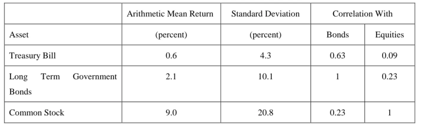
To illustrate the Properties demonstrated in Section IV, as well as the Asset Allocation Puzzle that arises from the misinterpretation of the Mutual Fund Theorem, we use the same example as in Canner, Mankiew and Weil (2001). The authors use historical data from 1926 to 1992 for the returns, volatilities and correlations of Treasury Bills, Long Term Government Bonds and Common Stock as shown in Table 1 below:
Table 1: Historical Data from Canner, Mankiew and Weil (2001)
Arithmetic Mean Return Standard Deviation Correlation With
Asset (percent) (percent) Bonds Equities
Treasury Bill 0.6 4.3 0.63 0.09
Long Term Government Bonds
2.1 10.1 1 0.23
Common Stock 9.0 20.8 0.23 1
Throughout the analysis, it is assumed that the leverage of the portfolio is k =1.
a) No Riskless Security
Assuming the return-risk coefficient to be equal to U´1/(-2U´2) = (1/5) and (U´1/(-2U´2)
= (1/4.4) , we would have the following allocations for Treasury Bills, Long Term Government Bonds and Common Stock in the Minimum Variance, Risk and Mean-Variance Efficient Portfolios:
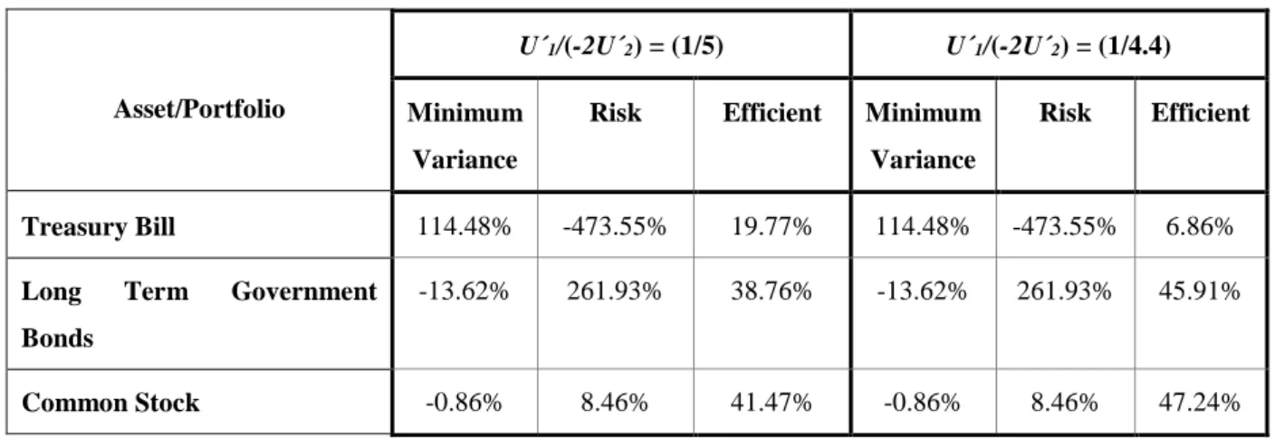
Table 2: Allocations in Minimum Variance, Risk and Optimal Portfolios for different U´1/(-2U´2)
Asset/Portfolio
U´1/(-2U´2) = (1/5) U´1/(-2U´2) = (1/4.4)
Minimum Variance
Risk Efficient Minimum
Variance
Risk Efficient
Treasury Bill 114.48% -473.55% 19.77% 114.48% -473.55% 6.86%
Long Term Government
Bonds
-13.62% 261.93% 38.76% -13.62% 261.93% 45.91%
Common Stock -0.86% 8.46% 41.47% -0.86% 8.46% 47.24%
There are four things to notice about Table 2. First of all, as demonstrated in Properties 5, 6 and 7, all the investment is allocated in the Minimum Variance Portfolio - whose allocation coefficients sum up to one - and none is allocated in the Risk Portfolio, which is completely self-financed and whose allocation coefficients sum up to zero. In other words, the Risk Portfolio is a tactical overlay portfolio and, for the specific cases analyzed in Table 2, it is comprised of an underweight in Treasury Bills that completely matches up the over-weights in Long Term Government Bonds and Common Stock.
Secondly, notice that all assets have an important contribution to both the Minimum Variance as well as the Risk Portfolios. As expected, the Treasury Bill comprises most of the allocation of the Minimum Risk Portfolio (actually a leveraged 114.48% allocation), while both Long Term Bonds (-13.62%) and Common Stock (-0.86%) contribute with small shorts to finance the leveraged position in the Treasury Bill.
Thirdly, as the Mutual Fund Theorem implies, the allocation of securities in both the Minimum Variance as well as the Risk Portfolios are independent of the return-risk preferences U´1/(-2U´2). However, something different happens in the Total Portfolio. There,
the magnitudes of the tactical allocation positions taken in the Risk Portfolio, are all adjusted by the return-risk coefficient U´1/(-2U´2). In particular, for the case in which the investor is
more risk-averse and U´1/(-2U´2) = (1/5), the Total Portfolio is comprised of 19.77% in
Treasury Bill, 38.76% in Long Term Government Bonds and 41.47% in Common Stock. However, for the case in which the investor is less risk-averse and U´1/(-2U´2) = (1/4.4), the
while the proportion of Stocks increases by 5.77 points, to 47.24% - both of these financed by a decrease exposure in the Treasury Bill of 12.91 percentage points, to 6.86%
That is, and this is the fourth thing to notice about Table 2, while the security allocations within the Risk Portfolio (as well as the Minimum Variance Portfolio) are indeed independent of the return-risk preferences - as the Mutual Fund Theorem would imply - their allocation in the Total Portfolio is not; as demonstrated in Property 8. In fact, for a more risk-averse investors, with U´1/(-2U´2) = (1/5), the proportion of Long Term Bonds to Common
Stocks in the Total Portfolio is 48.32% while for less risk-averse investors with U´1/(-2U´2) =
(1/4.4), it increases by 103 basis points, to 49.29%.
This is exactly the Asset Allocation Puzzle. And notice that it arises from a misinterpretation of the Risk Portfolio as being comprised of only Long Term Bonds and Common Stocks. If this misinterpretation is corrected, and the Risk Portfolio is as defined in Properties 1, then the ratio of Bonds to Common Stocks would remain constant and there would be no Asset Allocation Puzzle. This is also illustrated in Table 2.
b) Riskless Security
Let´s now redo the calculations for the case in which the Treasury Bill is a riskless security, having zero variance and zero covariance with Long Term Bonds and Common Stock. In this specific case, the allocations for the Minimum Variance, the Risk and the Mean-Variance Efficient Portfolios are illustrated in Table 3 below; for the cases in which the return-risk coefficients are, respectively, U´1/(-2U´2) = (1/5) and U´1/(-2U´2) = (1/4.4).
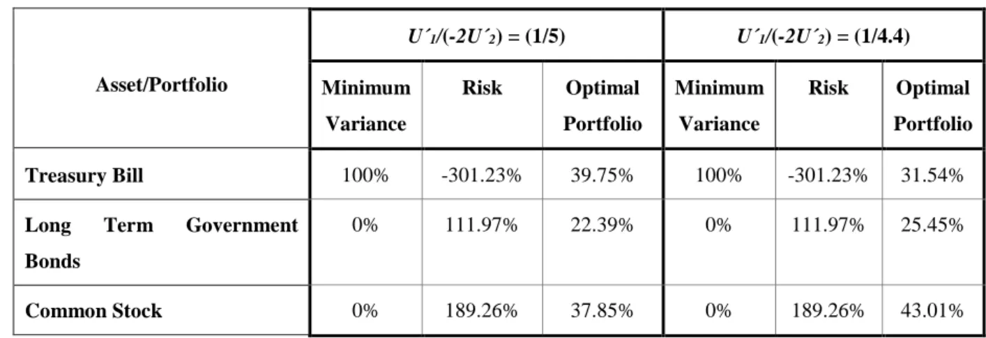
Table 3: Allocations in Minimum Variance, Risk and Optimal Portfolios for different U´1/(-2U´2)
for the case in which the Treasury Bill is riskless
Asset/Portfolio
U´1/(-2U´2) = (1/5) U´1/(-2U´2) = (1/4.4)
Minimum Variance Risk Optimal Portfolio Minimum Variance Risk Optimal Portfolio Treasury Bill 100% -301.23% 39.75% 100% -301.23% 31.54%
Long Term Government
Bonds
0% 111.97% 22.39% 0% 111.97% 25.45%
There are two things to notice about Table 3. The first one is that, as demonstrated in Property 4, if there is a Riskless Security, then the Minimum Variance allocation will be one for this security and zero for all other securities. That is, in this specific example, the Minimum Variance allocation in the Treasury Bill would be one and the Minimum Variance Allocations in Long Term Government Bonds and Common Stock would be zero.
The second thing to notice is that, if the Minimum Risk Allocation of Long Term Bonds and Common Stock are zero, then the proportion of Bonds to Stocks in the Risk Portfolio will be the same as the proportion of Bonds to Stocks in the Total Portfolio, as shown in Property 8. And, in fact, since the Mutual Fund Theorem implies that the proportion of Bonds to Stocks in the Risk Portfolio should be independent of the risk-return preferences, the same would also apply to the Total Portfolio. This is illustrated in Table 3 above, with the proportion of Long Term Bonds to Common Stock remaining at 37.17% for both the Risk as well as the Total Portfolios, independently on whether U´1/(-2U´2) = (1/5) or U´1/(-2U´2) =
(1/4.4). That is, in the presence of a Riskless security, the proportion of Bonds to Stocks would be constant even if one misinterpreted the Risk Portfolio as being comprised of only Bonds and Stocks. As this fact does not happen in practice, it ended up being interpreted in the Finance literature as an Asset Allocation puzzle.
c) Comparing the Two Procedures
Let´s now compare the two procedures mentioned in the paper. The first one, traditionally carried out in the Finance literature, starts by eliminating the Riskless Security from the Total Portfolio of N securities and then calculating a new “Risk” Portfolio of N – 1 risk securities. As a final step, it solves an Asset Allocation exercise to determine the optimal allocation between the Riskless Security and this new N – 1 “Risk” Portfolio. We will call this procedure “Traditional”.
The second procedure, as described in Section III, rewrites the first order conditions for the investor´s problem in such a way that the coefficient matrix can actually be inverted. This allows for the jointly determination of the Mean Variance Efficient allocation for the
Riskless Security as well as the N - 1 Risk Securities in the Portfolio. We call this procedure, “Jointly Determination”.
Table 4 below illustrates the Mean-Variance Efficient allocations that would arise from these two different procedures, for the case in which the Treasury Bill is the Riskless Security and the return-risk parameter is either U´1/(-2U´2) = (1/5) or U´1/(-2U´2) = (1/4.4).
Similar results would hold in the absence of a Riskless security; namely, the two procedures would yield different results.
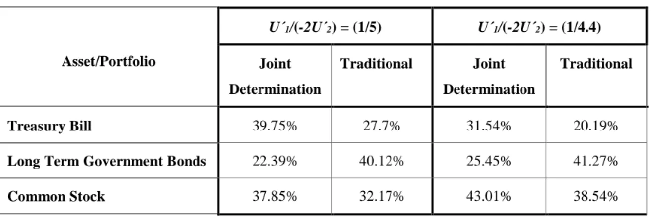
Table 4: Asset Allocations under the Joint determination of all Assets and under the Two Stages Procedure, for different U´1/(-2U´2) and for the case in which the Treasury Bill is riskless
Asset/Portfolio
U´1/(-2U´2) = (1/5) U´1/(-2U´2) = (1/4.4)
Joint Determination Traditional Joint Determination Traditional Treasury Bill 39.75% 27.7% 31.54% 20.19%
Long Term Government Bonds 22.39% 40.12% 25.45% 41.27%
Common Stock 37.85% 32.17% 43.01% 38.54%
There are two things to notice about Table 4. The first one is that, as suggested by Property 9, even for the case in which there exists a Riskless Security, both procedures will yield very different solutions to the investor problem. In other words, to jointly determine the allocation of N assets, as it is done in Section III, yields a different solution than to first solve the problem for N – 1 securities, and then solve an asset allocation problem between the remaining one security and the Efficient Portfolio of those N – 1 Securities - as it is done in the traditional Finance Literature. And a different solution exists even under the simplifying assumption that there exists a Riskless Security, as illustrated in Table 4.
Secondly, as shown in Properties 8 and 9, when there exists a Riskless Security, the proportion of Equities to Bonds in the Total Portfolio will be independent of the return-risk parameter under the Joint Determination Procedure; but it will not be independent under the Traditional Procedure. This is illustrated in Table 4. In fact, notice that for the Joint Determination procedure, the ratio of Bonds to Equities is 37.17% for U´1/(-2U´2) = (1/5) as
well as for U´1/(-2U´2) = (1/4.4). However, under the traditional procedure, the ratio of Bonds
to Equities would be 55.5% for U´1/(-2U´2) = (1/5) and 51.7% for the less risk averse investor
with U´1/(-2U´2) = (1/4.4). That is, even in the traditional two-steps procedure, an Asset
Allocation Puzzle would only exist if one misinterpreted the new “Risk” Portfolio as being comprised of only Bonds and Stocks.
I
I
.
.
C
C
o
o
n
n
c
c
l
l
u
u
s
s
i
i
o
o
n
n
This paper revisits the Mutual Fund Theorem using a different interpretation of the Risk Portfolio. Under this interpretation, the Risk Portfolio is a tactical overlay portfolio in which the overweight and underweight positions exactly cancel each other out. In this sense, the Risk Portfolio is completely self-financed and all investment is allocated to the Minimum Variance Portfolio; with differences in risk aversion resulting in no changes whatsoever in the Asset Allocation between the Minimum Variance and the Risk Portfolio - but rather in a tactical adjustment to the overweight and underweight positions within the Risk Portfolio. Such new interpretation of the Mutual Fund Theorem arises naturally for the case in which the first order conditions for the investor´s problem are written in a slightly different manner – that allows for the coefficient matrix to be inverted even in the presence of a Riskless Security.
In this sense, the Asset Allocation puzzle, as traditionally stated in the Finance textbooks, arises from a misinterpretation of what the facto is the Risk Portfolio. What happens is that, by the Mutual Fund Theorem, the Risk Portfolio is not comprised exclusively of risk assets such as Bonds and Stocks - as traditionally stressed - but rather of all securities in the Portfolio; including the Riskless Security. And once this is clarified, there is no Asset Allocation puzzle whatsoever. The dependence on the risk-return parameter that is observed in the data, of the ratio of Bonds to Stocks in the Total Portfolio, is exactly what is predicted by the Mutual Fund Theorem in the absence of a Riskless Security.
R
R
e
e
f
f
e
e
r
r
e
e
n
n
c
c
e
e
s
s
Canner, N.; G. Mankiw and D. Weil (1997): “As Asset Allocation Puzzle”. American Economic Review, March, pps. 181-191.
Elton, E.; M. Gruber and S. Brown (2009): “Modern Portfolio Theory and Investment Analysis”. John Wiley & Sons
Ingersoll, J. [1987]: “Theory of Financial Decision Making”. Rowman & LittleField Publishers Inc.
Merton, R. [1972]: “An Analytical Derivation of the Efficient Portfolio Frontier”. Journal of Financial and Quantitative Analysis, Vol. 7, No. 4, September, pp. 1851-1872.