ORIGINAL ARTICLE
CITE AS: Andrade, M.S.; Gorgens, E.B.; Reis, C.R.; Cantinho, R.Z.; Assis, M.; Sato, L.; Ometto, J.P.H.B. 2018. Airborne laser scanning for terrain modeling in the Amazon forest. Acta Amazonica 48: 271-279.
Airborne laser scanning for terrain modeling in the
Amazon forest
Mariana Silva ANDRADE1, Eric Bastos GORGENS1*, Cristiano Rodrigues REIS1,
Roberta Zecchini CANTINHO2, Mauro ASSIS3, Luciane SATO3, Jean Pierre Henry Balbaud OMETTO3
1 Universidade Federal dos Vales do Jequitinhonha e Mucuri - UFVJM, Departamento de Engenharia Florestal, Rodovia MGT 367 - Km 583, nº 5000, Alto da Jacuba,
CEP 39100-000, Diamantina, Minas Gerais, , Brasil
2 Ministério da Ciência, Tecnologia, Inovações e Comunicações. United Nations Development Programme. SCRN 702/703, 47, Asa Norte, CEP 70720-610, Brasília,
Distrito Federal, Brasil
3 Instituto Nacional de Pesquisas Espaciais - INPE, Centro de Ciências do Sistema Terrestre, Av. dos Astronautas, 1758, Jardim da Granja, CEP 12227-010, São José dos
Campos, São Paulo, Brasil
* Corresponding author: [email protected]
ABSTRACT
Very few studies have been devoted to understanding the digital terrain model (DTM) creation for Amazon forests. DTM has a special and important role when airborne laser scanning is used to estimate vegetation biomass. We examined the influence of pulse density, spatial resolution, filter algorithms, vegetation density and slope on the DTM quality. Three Amazonian forested areas were surveyed with airborne laser scanning, and each original point cloud was reduced targeting to 20, 15, 10, 8, 6, 4, 2, 1, 0.75, 0.5 and 0.25 pulses per square meter based on a random resampling process. The DTM from resampled clouds was compared with the reference DTM produced from the original LiDAR data by calculating the deviation pixel by pixel and summarizing it through the root mean square error (RMSE). The DTM from resampled clouds were also evaluated considering the level of agreement with the reference DTM. Our study showed a clear trade-off between the return density and the horizontal resolution. Higher forest canopy density demanded higher return density or lower DTM resolution.
KEYWORDS: ground filter, airborne LiDAR, digital terrain model, DTM, ALS
Escaneamento laser aerotransportado para modelagem de terreno em
floresta amazônica
RESUMO
São poucos os estudos dedicados a entender a criação de modelo digital de terreno (MDT) para florestas amazônicas. O MDT tem uma importante função quando o escaneamento laser aerotransportado é usado para estimar a biomassa da vegetação. Examinamos a relação da densidade de pulsos, resolução espacial, algoritmos de filtragem, densidade da vegetação e inclinação do terreno com a qualidade do MDT. Três áreas de floresta amazônica foram sobrevoadas usando LiDAR aerotransportado. Cada nuvem de dados original teve sua densidade reduzida objetivando 20; 15; 10; 8; 6; 4; 2; 1; 0,75; 0,5 e 0,25 pulsos por metro quadrado, utilizando um processo de reamostragem aleatória. Os MDTs das nuvens reamostradas foram comparados com o MDT de referência, produzido a partir da nuvem original, calculando o desvio pixel a pixel e resumindo-o por meio do erro padrão da estimativa (RMSE). Os MDTs das nuvens reamostradas também foram avaliados quanto ao nível de correspondência com o MDT de referência. Houve uma clara compensação entre densidade de pontos e resolução horizontal. Dosséis mais densos exigem uma maior densidade de retornos, ou MDT com menor resolução.
INTRODUCTION
Developing countries are concerned with the quantification of their forest carbon stocks, as part of the effort to negotiate carbon credits for emission reductions from deforestation and forest degradation (Saatchi et al. 2011). The Brazilian Reducing Emissions from Deforestation and Forest Degradation (REDD) initiative aims at defining a spatial carbon baseline and monitoring changes in forest stocks (Asner 2009). The IPCC framework imposes a regional or national mapping approach, which poses a huge challenge to the monitoring programs of developing countries (Asner et al. 2012a). REDD implementation is technically challenging in countries that have limited budgets to monitor extensive forests with complex and variable structure, in hardly accessible regions (Liu et al. 2007; Saatchi et al. 2011). Many studies have shown that Light Detection and Ranging (LiDAR) technology can contribute to tackle these challenges, generating spatially continuous high-resolution biomass information (Asner 2009; Saatchi et al. 2011; Asner et al.
2012b; Espírito-Santo et al. 2014).
Historically, large-scale carbon mapping relied on multispectral images and ground-based sample inventories (Saatchi et al. 2011). However, the multispectral-based approach presents problems in dealing with the complexity of tropical forest structures, which vary with climate, soil, vegetation and anthropogenic disturbances, among other factors (Lu et al. 2004; Sarker and Nichol 2011; Asner et al.
2012b). LiDAR deals well with forest structure complexity, due to its capacity to penetrate into the canopy (Lefsky et al.
1999). As a result, several projects aimed to estimate carbon stocks at regional or country level based on LiDAR technology, including Brazil (FUNCATE 2017), the Democratic Republic of the Congo (UCLA IoES 2017), Colombia (Asner et al.
2012a), and Malaysia (Coomes et al. 2017).
The standard approach consists in calibrating airborne LiDAR measurements against field-based biomass estimates. Many studies show that field-measured biomass estimates are consistently related to LIDAR measurements (Næsset 1997; Asner et al. 2012b). However, a reliable digital terrain model (DTM) is essential, since the LiDAR measurements used to describe the forest are based on vegetation height, which is obtained from the difference between the elevation of each laser return and the DTM (Næsset 1997; Lim and Treitz 2004; Asner et al. 2012a).
The challenge to create a good DTM is to filter the returns that truly reached the terrain from the LiDAR dataset (Meng
et al. 2010). However, finding the ground returns is not as simple as searching for the lowest returns in a given area. Distinguishing between ground and non-ground returns is particularly hard in regions with large relief variations, and in regions with dense vegetation cover (Meng et al. 2010; Hansen et al. 2015). To overcome these challenges, different
algorithms have been developed based on segmentation filters (Filin 2002), morphological filters (Arefi and Hahn 2005), contour based filters (Elmqvist 2002), triangulated irregular network filters (Axelsson 1999) and interpolation filters (Kraus and Pfeifer 1998; Kraus and Pfeifer 2001; Evans and Hudak 2007).
Misclassification of the ground returns commonly results in errors in the final DTM (Stereńczak and Kozak 2011). Many factors affect DTM accuracy, including density and distribution of the elevation sample, the filtering and interpolation algorithms, and the DTM resolution itself. The return density is a prerequisite to obtain very detailed high resolution (Liu et al. 2007) and it can be influenced by flight and sensor parameters, among others. Pulse density can be increased by increaseing the pulse rate frequency (PRF), increasing the scanning rate, overlapping flight paths, decreasing flight altitude, or decreasing the aircraft speed (individually or in combination). Usually, all parameters set to increase the pulse density also have a direct effect on the increase of acquisition costs (Jakubowski et al. 2013). LiDAR survey costs vary extensively. In the projects developed by our reasearch group, survey costs have varied from 4 R$/ ha to 250 R$/ha. Tilley et al. (2004) reported an equivalent variation, from US$1/ha to US$37/ha. Increasing the scale of area coverage and setting the flight parameters can reduce survey costs. In this context, very few studies have tried to understand the relationship between DTM accuracy, pulse density and filtering algorithms for tropical forests (Hansen
et al. 2015; Leitold et al. 2015; Jakubowski et al. 2013), and none has been carried out in the Amazon forest.
In this study we examined the relationship between pulse density, filter algorithm, and DTM accuracy in three areas of Amazon forest. We also investigated the influence of vegetation density and terrain complexity on DTM accuracy.
MATERIAL AND METHODS
Three high-density airborne laser scanning surveys were conducted over two forested areas located in the Brazilian Amazon region, characterized, respectively, by open and dense ombrophilous forest typologies. One flight was made over the Cauaxi Forest (Instituto Floresta Tropical) in the state of Pará (area 1, 3.76°S, 48.48°W), and two other flights over the Jamari National Forest, in the state of Rondônia (areas 2, 9.08°S, 62.80°W; and area 3, 9.14°S, 63.01°W) (Figure 1, Table 1). The areas have been managed under the reduced impact logging system. For more details about forest management procedures, refer to Monteiro et al. (2013) for Jamari Forest, and to Pinagé et al. (2015) for Cauaxi Forest.
413996 operating at a 100 kHz frequency. The scanning angle was 11°, with 65% of overlap between strips, and the flight altitude was about 850 m. This parameter setting resulted in a pulse density of ~ 10 pulses m-2 for a single scan and
~ 28 pulses m-2 for overlapping scans. The LIDAR sensor
was capable of recording up to four returns for each pulse, including last. The vendor processed the flight products using the PosPac, DashMap and TerraScan softwares. All data were projected using UTM SIRGAS 2000 for horizontal datum and Imbituba tide gauge station for vertical datum.
In the context of this study, it is important to distinguish between the concepts of pulse density and return density (also known as point density). The airborne LiDAR technology works by sending out short pulses of laser light downward from an airborne platform, which defines pulse density as the number of laser pulses per square meter sent out by the LiDAR equipment. The return density is defined as the number of returns registered from the backscattered energy of the emitted pulses (Baltsavia 1999). In practical terms, a single outgoing pulse may generate multiple returns, when there are partially transmitting strata of objects above the ground, such as the leaves and branches of trees.
The original LiDAR data were reduced targeting the following pulse densities: 20, 15, 10, 8, 6, 4, 2, 1, 0.75, 0.5 and 0.25 pulses m-2, based on a random resampling process.
The resampling algorithm computed the original pulse density Figure 1. Location of the three study areas in the Brazilian Amazon, in Cauaxi Forest (Pará state, PA, area 1) and Jamari National Forest (Rondônia state, RO, areas 2 and 3). Maps 1, 2 and 3 show the DTM derived from the original point cloud of each study area, respectively.
Table 1. Descriptive summary of the airborne laser scanning campaigns in our three study areas in the Brazilian Amazon, located in Cauaxi Forest (Pará state) (Area 1) and Jamari National Forest (Rondônia state) (Areas 2 and 3).
Area 1 Area 2 Area 3
Flight date 27 Jul 2012 20 Nov 2011 17 Nov 2011
UTM Zone 22S 20S 20S
Elevation (m above sea level) 84 - 148 83 - 118 86 - 108
High slope (degrees) 44 19.5 16.5
Average slope (degrees) 6.2 3.3 1.8
Total area (hectares) 1214 500 500
Average return density (returns m-²) 28.3 25.8 25.1
Average 1st returns density (returns m-²) 13.89 16.15 15.43
P50 (m) 22.7 19.5 20.8
Cover (%)1 81.3 77.1 78.5
Canopy Relief Ratio2 0.42 0.38 0.41
to a 25-by-25-meter window and randomly removed pulses to reach the target pulse density. Removing a pulse implicated removing all returns related to that pulse, and for that reason the resulting point density was not exactly the same value of the pulse density target. During the resampling process, a new pulse was identified whenever a first return was found or when there was an intermediate return without the previous level (e.g. second return without a first return). More details about the resampling process can be found in McGaughey (2013).
To filter the ground returns for DTM creation, three filtering algorithms were considered. Two were based on interpolation (Kraus and Pfeifer 1998, from now on referred to as KF; and Evans and Hudak 2007, from now on referred to as EH), and one was based on a triangulated irregular network (Axelsson 1999, from now on referred to as AX). The choice of the algorithms was guided by their availability in airborne laser scanning (ALS) processing software and their popularity among forest analysts. The KF algorithm was implemented in FUSION/LTK 3.5 and set considering an 8-meter window size (Silva et al. 2012) and standard filter parameters (McGaughey 2013). The EH algorithm was implemented in MCC-LiDAR 2.1 and parameterized considering the scale parameter of 1.5 and the curvature limit of 0.3, according to the software manual (Hudak 2016). The AX algorithm was implemented in LASTOOLS version 120628 and all the parameters set to standard values. We produced a series of DTMs in a full factorial scheme of algorithms with horizontal resolutions (1, 2, 5 and 10 meters) and pulse densities (20, 15, 10, 8, 6, 4, 2, 1, 0.75, 0.5 and 0.25 pulses m-2). From
here onward, we will refer to a DTM produced in this way as DTMres.
To ideally assess the DTMres accuracy, the produced surface should be compared with a “true” terrain surface, recorded by differential GPS, by a leveling station or by a total station (Liu
et al. 2007). In differential GPS acquisition, the georeferenced data is corrected using a static base station and post-processing, applying a proper geographic transformation. In theodolite or total station survey, the produced planimetric map should be georeferenced using some ground reference coordinates. In the Amazon, ground truth acquisition is technically constrained by the demands of great field effort and high costs (Rempel et al. 1995; Sigrist et al. 1999, Valbuena et al 2010). The implementation of ground surveys based on topographic equipment is logistically challenging in dense vegetation, due to factors such as limited field of view, high air moisture and temperature, and frequently inaccessible survey areas. Dense vegetation also influences GPS data collection by significantly increasing signal interruption and interference in the reception of the continuous array of epochs used to fix the phase ambiguity (Valbuena et al.
2010). The forest canopy also affects precision, mainly due to wave propagation interference, blocking or attenuating the signal and increasing the multipath effect (Monico 2007).
Such conditions substantially increase the recording time per point (Valbuena et al. 2010) and positional errors can reach 3.5 m in horizontal, and 5 m in vertical position (Yoshimura and Hasegawa 2003). To overcome these problems, Liu et al. (2007) and Jakubowski et al. (2013) proposed the use of a DTM created from the highest return density cloud as a reference (DTMref). The DTMref will be used as a reference for DTMres. A total of 144 DTMs were created for each area (four resolutions x 12 pulse densities x three filter algorithms). To evaluate the deviation from the reference, each DTMres was compared to the DTMref,calculating the deviation pixel by pixel and summarizing the deviations as the root mean square error (RMSE). The comparison between DTMres and DTMref was carried outkeeping the resolution and the filter algorithm fixed, and using the effect size concept by means of Cohen’s d (Cohen 1988). Therefore the RMSE represented the accuracy loss caused by the pulse density reduction, and Cohen’s d measured the strength of the relationship between two surfaces on a numeric scale. The effect size estimates a population parameter and is not affected by sample size (Sawilowsky 2009).
For each study area, the DTMres with the highest effect size (i.e. with the largest difference relative to DTMref) was subtracted from the respective DTMref by computing the deviation. The influence of vegetation density and slope on the deviation was analyzed through a scatterplot. Forest canopy cover is a projection of the vertical profile of canopy foliage onto a horizontal plane (Smith et al. 2009). As a proxy for vegetation density, we used the ratio between the number of returns above 10 m and the total number of returns, further referenced as cover (in %) (Smith et al. 2009; Hopkinson and Chasmer 2009). The slope was defined as the angle of inclination to the horizontal. All the analyses was performed in R version 3.1.1 using the raster, rgdal, and effsize packages.
RESULTS
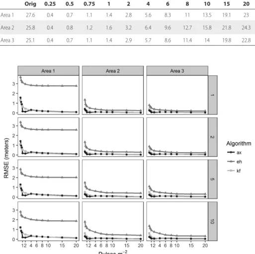
Even considering the same pulse density target, the final return density for each cloud was not exactly the same, due to the resampling algorithm employed (Table 2). The RMSE was higher for DTMres derived from the 0.25 pls m−2 clouds and
reduced logarithmically as the pulse density increased. AX and KF showed very similar performance, and EH the highest RMSE values (Figure 2). A high-resolution DTM required a higher pulse density to warrant a sub-metric RMSE. In area 1, AX was able to create a 1m-resolution DTMres from a 10 pulses m−2 cloud with an RMSE of 0.17 m. Considering
a lower-resolution, the 0.75 pulses m−2 cloud generated a
DTMres with RMSE of 0.67 m.
0 and 0.099117. A transect from area 1 exemplifies the small effect size, that indicates a very strong relationship between the two surfaces on a numeric scale (Figure 3).
Area 1 had the most complex terrain among the study areas. AX and KF showed sub-metric RMSE for DTMres produced from 0.75 and 0.5 pulses m-2 clouds, respectively.
The DTMres produced with EH never reached RMSE values below 1.5 (Figure 2). For areas 2 and 3, all three algorithms performance better with respect to RMSE than for area 1. However, AX and KF still performed better then EH.
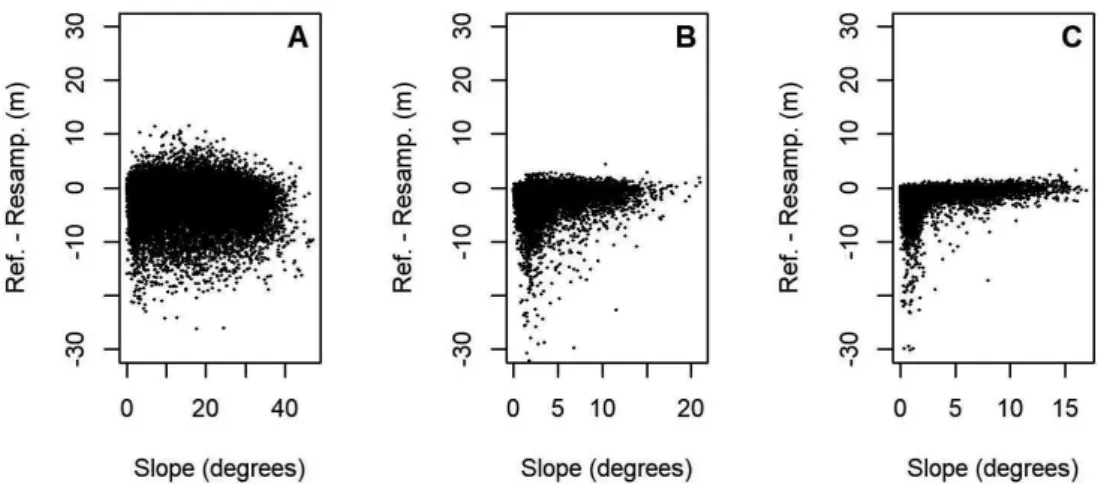
The DTMres with the highest effect size for area 1 was the 5m-resolution model created with AX from the 0.25 pulses m−2 cloud. For areas 2 and 3, the highest effect size
was obtained for the 10 m-resolution DTMres created with EH from the 0.25 pulse m−2 cloud. The plot of the deviation
between DTMres and DTMref suggested that deviations increased with cover percentage (Figure 4). The plots of deviations against slope showed a decrease of deviations when slope increased (Figure 5). AX and KF showed very similar performance for all study areas. AX returned smaller RMSE than KF, but KF showed a smaller effect size.
DISCUSSION
The DTM analysis of three types of vegetation in Malaysia showed errors varying from 0.24 m to 3.06 m for mixed tropical forest areas when compared to ground returns, with lower errors associated with the high point-density derived DTMs (Rasib et al. 2013). In Brazilian Atlantic Forest, differences up to 3.02 m were observed between the DTM from the resampled LAS files (1 pulse m−2) and the control
Figure 2. Root mean square error (RMSE) of digital terrain models (DTMs) derived from resampling of originally acquired airborne LiDAR data at different pulse densities (20, 15, 10, 8, 6, 4, 2, 1, 0.75, 0.5 and 0.25 pulses m−2) in three areas of Brazilian Amazon forest in Cauaxi Forest, in Pará state (Area 1) and Jamari National Forest,
in Rondônia state (Areas 2 and 3). Lines indicate resampling using different filter algorithms: Kraus and Pfeifer (KF) = light gray; Evans and Hudak (EH) = dark gray; and Axelsson (AX) = black. For each area resamplings are presented at spatial resolutions of 1, 2, 5 and 10 m
Table 2. Final return density (returns m-2) after resampling to targeting pulse densities of 0.25, 0.5, 0.75, 1, 2, 4, 6, 8, 10, 15 and 20 pulses m-2. of airborne LiDAR scanning
data in three study areas in the Brazilian Amazon [Cauaxi Forest (Pará state) (Area 1) and Jamari National Forest (Rondônia state) (Areas 2 and 3)]. Orig = original point cloud.
Targeting pulse density (pulses m-2)
Orig 0.25 0.5 0.75 1 2 4 6 8 10 15 20
Area 1 27.6 0.4 0.7 1.1 1.4 2.8 5.6 8.3 11 13.5 19.1 23
Area 2 25.8 0.4 0.8 1.2 1.6 3.2 6.4 9.6 12.7 15.8 21.8 24.3
Figure 3. Elevation profiles for a transect from area 1 (in Cauaxi Forest, Pará state). A - DTM derived from the 20 pulses m-2 cloud (in gray) and the reference (in black);
B - DTM derived form the 0.25 pulses m-2 cloud (in gray) and the reference (in black).
Figure 4. Difference between the digital terrain model (DTM) derived from the original cloud (Ref ) and the resampled (Resamp) clouds as a function of metric cover (%) in three study areas in the Brazilian Amazon. A - area 1 (Cauaxi Forest, in Pará state); B - area 2; and C - area 3 (Jamari National Forest, in Rondônia state).
points obtained in the field (Leitold et al. 2015). When compared to the DTM derived from the 20 pulses m-2 cloud,
the difference was 0.19 m. In both studies, the higher the return density of the cloud used to create the DTM, the smaller was the error compared to ground points. The RMSE range in our study (0.01 m to 3.67 m) was very similar to the observed by Rasib et al. (2013) and Leitold et al. (2015). Our results showed an interesting relation between spatial resolution, deviation from the DTMref and consistency of the DTMres. DTMres derived from lower pulse density clouds showed larger RMSE and a larger effect size. Consistency refers to similar surfaces comparing DTMres and the respective DTMref. LiDAR datasets can withstand substantial data reduction without reducing the DTM quality, but the level of data reduction is significantly influenced by the desired horizontal resolution (Guo et al. 2010). Density reduction can increase the efficiency of DTM generation due to smaller file size and less processing time, but it depends on the terrain characteristics, the interpolation method, and data resolution (Liu et al. 2007). For tree plantations, an increase in return density produced little improvement in the volume estimation accuracy (Tesfamichael et al. 2010).
The lower performance of EH was unexpected since this algorithm was developed for high-biomass and high-relief areas (Evans and Hudak 2007). As we kept the algorithm parameters as suggested by the authors, there is a chance that EH performance can be improved in our survey areas by fine-tuning the parameter settings. On the other side, no single algorithm can perform well in all kinds of situations (Maguya et al. 2014).
The influence of slope was not as strong as that of the forest cover on DTM extraction in our study. Contrary to our results, in a tropical forest in Costa Rica, a comparison between ground control points and a DTM derived from a 9 pulses m−2 cloud indicated larger errors in areas with greater
slope (Clark et al. 2004). Slope was not very accentuated in our study areas, so that other factors, which were not controlled in our study, such as season (which affects leaf density), scan angle, and flight altitude could have influenced response to slope (Maguya et al. 2014). Yet, in the Costa Rica forest, DTM error was also larger in areas of dense forest canopy when keeping the relief constant (Clark et al. 2004). Forest canopy density was also positively correlated with DTM error in a coniferous forest in western North America (Reutebuch et al.
2003). Dense vegetation has been recognized as an important drawback to generate accurate DTM, as it blocks the pulse pathway (Hansen et al. 2015; Leitold et al. 2015). An increase in pulse density in areas of dense canopy may increase the probability of pulses reaching the ground (Meng et al. 2010). New algorithms are being developed for terrain extraction from airborne laser scanning (Cheng et al. 2017). However, few of them are so far available as commercial software, and
others do not have yet an end-user interface implemented. As new algorithms become available, it is important to compare their performance with that of algorithms that have been in use for a longer time, in order to support users in their decision-making process. The use of airborne scanning to monitor tropical forests is becoming more popular, which demands a better understanding of the available processing alternatives and the consequences for product generation.
CONCLUSIONS
Our study showed that it is possible to produce consistent DTMs from low-density LiDAR clouds in areas of Amazon forest in Rondônia and Pará (northern Brazil). Among the three selected filters, the Kraus and Pfeifer filter was the most efficient to extract the DTM in our three study areas. There was a trade-off between pulse density and DTM quality. Though the DTM was still consistent with lower point density, its accuracy decreased. It was possible to reduce the observed differences by decreasing the horizontal resolution of the DTM. Our work indicates that, by optimizing flight parameters, it is possible to increase the accuracy of DTMs in large-scale projects of forest monitoring in the Amazon region.
ACKNOWLEDGMENTS
This study was supported by Fundo Amazônia (Banco Nacional de Desenvolvimento Econômico e Social - BNDES) (processo: 14.2.0929.1) and by Conselho Nacional de Desenvolvimento Científico e Tecnológico - CNPq, chamada Universal (processo 403297/2016-8). We also thank the Instituto Nacional de Pesquisas Espaciais - INPE, the Universidade Federal dos Vales do Jequitinhonha e Mucuri - UFVJM, the Fundação de Amparo à Pesquisa do Estado de Minas Gerais - FAPEMIG and the Coordenação de Aperfeiçoamento de Pessoal de Nível Superior - CAPES. The ALS data was provided by Projeto Paisagens Sustentáveis (US Forest Service and Empresa Brasileira de Pesquisa Agropecuária - Embrapa).
REFERENCES
Arefi, H.; Hahn, M. 2005. A morphological reconstruction algorithm for separating off-terrain points from terrain points in laser scanning data. International Archives of Photogrammetry, Remote
Sensing and Spatial Information Sciences, 36: 120-125.
Asner, G.P.; Clark, J.K.; Mascaro, J.; Galindo-García, G.A.; Chadwick, K.D.; Navarrete-Encinale, D.A.; et al. 2012. High-resolution mapping of forest carbon stocks in the Colombian Amazon. Biogeosciences, 9: 2683-2696.
Asner, G.P. 2009. Tropical forest carbon assessment: integrating satellite and airborne mapping approaches. Environmental
Research Letters, 4: 034009.
A universal airborne lidar approach for tropical forest carbon mapping. Oecologia, 168: 1147-1160.
Axelsson, P. 1999. Processing of laser scanner data—algorithms and applications. ISPRS Journal of Photogrammetry and Remote
Sensing, 54: 138-147.
Baltsavias, E.P. 1999. Airborne laser scanning: basic relations and formulas. ISPRS Journal of Photogrammetry and Remote
Sensing, 54: 199–214.
Chen, Z.; Gao, B.; Devereux, B. 2017. State-of-the-Art: DTM Generation Using Airborne LIDAR Data. Sensors, 17:24.
Clark, M.L.; Clark, D.B.; Roberts, D.A. 2004. Small-footprint lidar estimation of sub-canopy elevation and tree height in a tropical rain forest landscape. Remote Sensing of Environment, 91: 68-89. Cohen, J. 1988. Statistical power analysis for the behavioral sciences.
2nd ed., Erlbaum Associates, Hillsdale, 579p.
Coomes, D.A.; Dalponte, M.; Jucker, T.; Asner, G.P.; Banin, L.F.; Burslem, D.F.R.P.; et al. 2017. Area-based vs tree-centric approaches to mapping forest carbon in Southeast Asian forests from airborne laser scanning data. Remote Sensing of Environment, 194: 77-88.
Elmqvist, M. 2002. Ground surface estimation from airborne laser scanner data using active shape models. International Archives of
Photogrammetry Remote Sensing and Spatial Information Sciences,
34: 114-118.
Espírito-Santo, F.D.; Gloor, M.; Keller, M.; Malhi, Y.; Saatchi, S.; Nelson, B.; et al. 2014. Size and frequency of natural forest disturbances and the amazon forest carbon balance. Nature
Communications, 5: 3434.
Evans, J.S.; Hudak, A.T. 2007. A multiscale curvature algorithm for classifying discrete return lidar in forested environments. IEEE
Transactions on Geoscience and Remote Sensing, 45: 1029-1038.
Filin, S. 2002. Surface clustering from airborne laser scanning data.
International Archives of Photogrammetry Remote Sensing and
Spatial Information Sciences, 34: 119-124.
FUNCATE. 2017. Monitoramento Ambiental por Satélite no Bioma Amazônia (https://www.funcate.org.br/msa/projetos/mudanca-de-uso-da-terra/). Accessed on 14/05/2018.
Guo, Q.; Li, W.; Yu, H.; Alvarez, O. 2010. Effects of topographic variability and lidar sampling density on several dem interpolation methods. Photogrammetric Engineering & Remote Sensing, 76: 701-712.
Hansen, E.H.; Gobakken, T.; Næsset, E. 2015. Effects of pulse density on digital terrain models and canopy metrics using airborne laser scanning in a tropical rainforest. Remote Sensing, 7: 8453-8468.
Hopkinson, C.; Chasmer, L. 2009. Testing lidar models of fractional cover across multiple forest ecozones. Remote Sensing
of Environment, 113: 275-288.
Hudak, A. 2016. MCC-LiDAR: (https://sourceforge.net/p/mcclidar/ wiki/Home). Acesso em 10/10/2016.
Jakubowski, M.K.; Guo, Q.; Kelly, M. 2013. Tradeoffs between lidar pulse density and forest measurement accuracy. Remote Sensing
of Environment, 130: 245-253.
Kraus, K.; Pfeifer, N. 1998. Determination of terrain models in wooded areas with airborne laser scanner data. ISPRS Journal of
Photogrammetry and Remote Sensing, 53: 193-203.
Kraus, K.; Pfeifer, N. 2001. Advanced dtm generation from lidar data. TheInternational Archives of Photogrammetry, Remote Sensing
and Spatial Information Sciences, 34: 23-30.
Lefsky, M.A.; Cohen, W.B.; Acker, S.A.; Parker, G.G.; Spies, T.A.; Harding, D. 1999. Lidar remote sensing of the canopy structure and biophysical properties of douglas-fir western hemlock forests.
Remote Sensing of Environment, 70: 339-361.
Leitold, V.; Keller, M.; Morton, D.C.; Cook, B.D.; Shimabukuro, Y.E. 2015. Airborne lidar-based estimates of tropical forest structure in complex terrain: opportunities and trade-offs for REDD+. Carbon Balance and Management, 10: 3.
Lim, K.S.; Treitz, P.M. 2004. Estimation of above ground forest biomass from airborne discrete return laser scanner data using canopy-based quantile estimators. Scandinavian Journal of Forest
Research, 19: 558-570.
Liu, X.; Zhang, Z.; Peterson, J.; Chandra, S. 2007. The effect of lidar data density on DEM accuracy. Proceedings of the International
Congress on Modelling and Simulation, p.1363-1369.
Lu, D.; Mausel, P.; Brondízio, E.; Moran, E. 2004. Relationships between forest stand parameters and Landsat TM spectral responses in the Brazilian Amazon Basin. Forest Ecology and
Management, 198: 149–167.
Maguya, A.S.; Junttila, V.; Kauranne, T. 2014. Algorithm for extracting digital terrain models under forest canopy from airborne lidar data. Remote Sensing, 6: 6524-6548.
Mcgaughey, R. 2013. Fusion/LDV: Software for lidar data analysis
and visualization. 3.3 ed. USDA Forest Service, Portland. 211p.
Meng, X.; Currit, N.; Zhao, K. 2010. Ground filtering algorithms for airborne lidar data: A review of critical issues. Remote Sensing, 2: 833-860.
Monteiro, A.L.S.; Cruz, D.C.; Cardoso, D.R.S.; Souza Jr, C.M. 2013. Monitoramento remoto de concessões florestais na amazônia - flona do Jamari, Rondônia. Anais do XVI Simpósio
Brasileiro de Sensoriamento Remoto,p.6433-6440.
Næsset, E. 1997. Estimating timber volume of forest stands using airborne laser scanner data. Remote Sensing of Environment, 61: 246-253.
Pinagé, E.R.; Keller, M.; Dos-Santos, M.N.; Spinelli-Araújo, L.; Longo, M. 2015. Avaliação temporal dos efeitos da exploração madeireira usando dados lidar. Anais do XVII Simpósio Brasileiro
de Sensoriamento Remoto, p.834-841.
Rasib, A.W.; Ismail, Z.; Rahman, M.Z.A.; Jamaluddin, S.; Kadir, W.H.W.; Ariffin, A.; Razak, K.A.; Kang, C.S. 2013. Extraction of digital terrain model (dtm) over vegetated area in tropical rainforest using lidar. Proceedings of the IEEE, Geoscience and
Remote Sensing Symposium, p.3391-3394.
Monico, J.F.G. 2007. Posicionamento pelo GNSS: descrição,
fundamentos e aplicações, 2nd ed. Editora UNESP, Botucatu,
480p.
Rempel, R.S.; Rodgers, A.R.; Abraham, K.F. 1995. Performance of a GPS animal location system under boreal forest canopy. The
This is an Open Access article distributed under the terms of the Creative Commons Attribution License, which permits unrestricted use, distribution, and reproduction in any medium, provided the original work is properly cited.
Reutebuch, S.E.; Mcgaughey, R.J.; Andersen, H.E.; Carson, W.W. 2003. Accuracy of a high-resolution lidar terrain model under a conifer forest canopy. Canadian Journal of Remote Sensing, 29: 527-535.
Saatchi, S.S.; Harris, N.L.; Brown, S.; Lefsky, M.; Mitchard, E. T.; Salas, W.; et al. 2011. Benchmark map of forest carbon stocks in tropical regions across three continents. Proceedings of the
National Academy of Sciences, 108: 9899-9904.
Sarker, L.R.; Nichol, J.E. 2011. Improved forest biomass estimates using ALOS AVNIR-2 texture indices. Remote Sensing of
Environment, 115: 968-977.
Sawilowsky, S.S. 2009. New effect size rules of thumb. Journal of
Modern Applied Statistical Methods, 8: 597-599.
Sigrist, P.; Coppin, P.; Hermy, M. 1999. Impact of forest canopy on quality and accuracy of gps measurements. International Journal
of Remote Sensing, 20: 3595-3610.
Silva, A.G.P.; Gorgens, E.B.; Rodriguez, L.C.E.; Silca, C.A.; Alvares, C.A.; Campoe, O.C.; Stape, J.L. 2012. Influência da janela do filtro de terreno em dados lidar sob duas coberturas florestais.
Anais do X Seminário de Atualização em Sensoriamento Remoto e Sistemas de Informações Geográficas Aplicados à Engenharia Florestal, p.65-72.
Smith, A.M.; Falkowski, M.J.; Hudak, A.T.; Evans, J.S.; Robinson, A.P.; Steele, C.M. 2009. A cross-comparison of field, spectral, and lidar estimates of forest canopy cover. Canadian Journal of
Remote Sensing, 35: 447–459.
Stereńczak, K.; Kozak, J. 2011. Evaluation of digital terrain models generated in forest conditions from airborne laser scanning data acquired in two seasons. Scandinavian Journal of Forest Research, 26: 374-384.
Tesfamichael, S.; Ahmed, F.; Aardt, J.V. 2010. Investigating the impact of discrete-return lidar point density on estimations of mean and dominant plot-level tree height in eucalyptus grandis plantations. International Journal of Remote Sensing, 31: 2925-2940.
Tilley, B.K.; Munn, I.A.; Evans, D.L.; Parker, R.C.; Roberts, S.D. 2004. Cost considerations of using lidar for timber inventory.
Proceedings of the Southern Forest Economics Workers, p.43-50.
UCLAS IoES. 2017. Carbon map of DRC: High resolution carbon
distribution in forests of Democratic Republic of Congo. University
of California, Institute of the Environment and Sustainability, Los Angeles,64p.
Valbuena, R.; Mauro, F.; Rodriguez-Solano, R.; Manzanera, J.A. 2010. Accuracy and precision of GPS receivers under forest canopies in a mountainous environment. Spanish Journal of
Agricultural Research, 8: 1047-1057.
Yoshimura, T.; Hasegawa, H. 2003. Comparing the precision and accuracy of GPS positioning in forested areas. Journal of Forest
Research, 8: 147-152.
RECEIVED: 15/01/2018
ACCEPTED: 22/08/2018