UNIVERSIDADE NOVA DE LISBOA
Faculdade de Ciências e Tecnologia
Departamento de Química
Experimental design methodologies
for the identification of
Michaelis-Menten type kinetics
Por
Filipe Ataíde
Dissertação apresentada na Faculdade de Ciências e Tecnologia da
Universidade Nova de Lisboa para obtenção do grau de Mestre em
Acknowledgements
First of all, I would like to thank my family, especially my parents, for supporting me in
such a way that I could spend 6 months in Hannover (Germany) to elaborate my Master
thesis;
To Prof. Bernd Hitzmann and Prof. Rui Oliveira, regarding the thesis coordination and
support;
To all the elements of Bernd Hitzmann’s work group, in particular to Patrick Lindner
and David Geissler, for all the help provided with Matlab software, during my stay in
Hannover;
To my new friends from Erasmus, with a special word to Asia, Petra and Joana;
To all my good friends that made the distance bearable and showed me how important
they really are in my life;
And last, but not least, Fábio, who was there for me in every single moment and shared
both Erasmus and Master thesis’ experience with me.
To all of you,
Table of Contents
1. Introduction ... 2
2. System and Methods... 3
2.1. Calculation of the Fisher Information Matrix ... 3
2.2. Experimental design optimality criteria ... 5
2.2.1 A-criterion ... 5
2.2.2 D-criterion ... 6
2.2.3 E-criterion... 6
2.2.4 Modified E-criterion ... 7
2.3. Genetic Algorithm ... 7
3. Process and implementation details... 9
3.1. Experiment description... 9
3.2. Process restrictions and possible design scheme... 10
3.3. Measurement error variances... 13
3.4. Conditions for the comparison between experimental design and equidistant sampling ... 14
4. Results and Discussion ... 14
4.1. Experimental design for batch process ... 14
4.2. Experimental design for fed-batch (pulses) process... 17
4.3. Experimental design for fed-batch (continuous) process ... 19
4.4. Equidistant sampling for batch and fed-batch (pulses) processes ... 21
4.5. Comparison between experimental design and equidistant measurement points for batch process ... 22
4.6. Comparison between experimental design and equidistant sampling for fed-batch (pulses) process ... 26
Table of Figures
Figure 2.1: Diagram of genetic algorithm’s simplified way of working... 8
Figure 3.1: Example of optimized time tag points for continuous feed and an adjusted
function that will represent the feeding rate throughout the experiment... 12
Figure 4.1: Substrate concentration and squared sensitivities of the batch process using
criterion A and error 1, for experimental design... 15
Figure 4.2: Quotient between Sv2
( )
timax and SKm
( )
ti 2and profile of substrate concentration
through time... 16
Figure 4.3: Substrate concentration and squared sensitivities of the optimized fed-batch
(pulses) process using criterion A and error 1, for experimental design ... 18
Figure 4.4: Substrate concentration and squared sensitivities of the optimized fed-batch
(continuous) process using criterion A and error 1, for experimental design... 20
Figure 4.5: Substrate concentration and squared sensitivities of the fed-batch (pulses)
process using criterion A and error 1 for equidistant sampling’ method... 22
Figure 4.6: CRLB vmax dependence on real values of vmax for experimental design (Km
fixed to 0.3 mol/L) and equidistant sampling using 1, for batch process ... 24
Figure 4.7: CRLB Km dependence on real values of Km for experimental design (vmax
fixed to 0.12 mol/(g.h)) and equidistant sampling using 1, for batch process ... 24
Figure 4.8: CRLB vmax dependence on real values of vmax for experimental design (Km
fixed to 0.3 mol/L) and equidistant sampling using 1, for fed-batch (pulses) process . 27
Figure 4.9: CRLB Km dependence on real values of Km for experimental design (vmax
fixed to 0.12 mol/(g.h)) and equidistant sampling using 1, for fed-batch (pulses)
process ... 27
Figure 8.1: Results for experimental design - batch mode, criterion A and error 1...II
Figure 8.2: Results for experimental design - batch mode, criterion A and error 2...III
Figure 8.3: Results for experimental design - batch mode, criterion D and error 1... IV
Figure 8.4: Results for experimental design - batch mode, criterion D and error 2...V
Figure 8.5: Results for experimental design - batch mode, criterion E and error 1... VI
Figure 8.6: Results for experimental design - batch mode, criterion E and error 2... VII
Figure 8.7: Results for experimental design - batch mode, criterion E-mod and error 1
Figure 8.8: Results for experimental design - batch mode, criterion E-mod and error 2
... IX
Figure 8.9: Results for experimental design – fed-batch mode (pulses), criterion A and
error 1...X
Figure 8.10: Results for experimental design – fed-batch mode (pulses), criterion A and
error 2... XI
Figure 8.11: Results for experimental design – fed-batch mode (pulses), criterion D and
error 1... XII
Figure 8.12: Results for experimental design – fed-batch mode (pulses), criterion D and
error 2...XIII
Figure 8.13: Results for experimental design – fed-batch mode (pulses), criterion E and
error 1... XIV
Figure 8.14: Results for experimental design – fed-batch mode (pulses), criterion E and
error 2...XV
Figure 8.15: Results for experimental design – fed-batch mode (pulses), criterion E-mod
and error 1... XVI
Figure 8.16: Results for experimental design – fed-batch mode (pulses), criterion E-mod
and error 2... XVII
Figure 8.17: Results for experimental design – fed-batch mode (continuous), criterion A
and error 1...XVIII
Figure 8.18: Results for experimental design – fed-batch mode (continuous), criterion A
and error 2... XIX
Figure 8.19: Results for experimental design – fed-batch mode (continuous), criterion D
and error 1...XX
Figure 8.20: Results for experimental design – fed-batch mode (continuous), criterion D
and error 2... XXI
Figure 8.25: Results for equidistant sampling – batch mode, criterion A and error 1
... XXVI
Figure 8.26: Results for equidistant sampling – batch mode, criterion A and error 2
... XXVII
Figure 8.27: Results for equidistant sampling – fed-batch (pulses) mode, criterion A and
error 1...XXVIII
Figure 8.28: Results for equidistant sampling – fed-batch (pulses) mode, criterion A and
error 2... XXIX
Figure 9.1: Comparison between experimental design and equidistant sampling - batch
mode, criterion A, 1... XXXI
Figure 9.2: Comparison between experimental design and equidistant sampling - batch
mode, criterion A, 2... XXXII
Figure 9.3: Comparison between experimental design and equidistant sampling - batch
mode, criterion D, 1...XXXIII
Figure 9.4: Comparison between experimental design and equidistant sampling - batch
mode, criterion D, 2...XXXIV
Figure 9.5: Comparison between experimental design and equidistant sampling - batch
mode, criterion E, 1... XXXV
Figure 9.6: Comparison between experimental design and equidistant sampling - batch
mode, criterion E, 2...XXXVI
Figure 9.7: Comparison between experimental design and equidistant sampling - batch
mode, criterion E-mod, 1... XXXVII
Figure 9.8: Comparison between experimental design and equidistant sampling - batch
mode, criterion E-mod, 2... XXXVIII
Figure 9.9: Comparison between experimental design and equidistant sampling –
fed-batch (pulses) mode, criterion A, 1...XXXIX
Figure 9.10: Comparison between experimental design and equidistant sampling –
fed-batch (pulses) mode, criterion A, 2... XL
Figure 9.11: Comparison between experimental design and equidistant sampling –
fed-batch (pulses) mode, criterion D, 1...XLI
Figure 9.12: Comparison between experimental design and equidistant sampling –
fed-batch (pulses) mode, criterion D, 2... XLII
Figure 9.13: Comparison between experimental design and equidistant sampling –
Figure 9.14: Comparison between experimental design and equidistant sampling –
Index of Tables
Table 3.1: Parameters and conditions used in the experiments... 13
Table 4.1: Results of the optimization for batch process using the error 1... 17
Table 4.2: Results of the optimization for batch process using error 2... 17
Table 4.3: Results of the optimization for fed-batch (pulses) process using the error 119
Table 4.4: Results of the optimization for fed-batch (pulses) process using the error 219
Table 4.5: Results of the optimization for fed-batch (continuous) process using the error
1... 21
Table 4.6: Results of the optimization for fed-batch (continuous) process using the error
2... 21
Table 4.7: Time tags for the equidistant sampling and its results ... 22
Table 4.8: Lowest CRLB’s and its corresponding parameter for experimental design and
range in which experimental design is better than equidistant sampling for batch process
using the error 1, for vmax... 24
Table 4.9: Lowest CRLB’s and its corresponding parameter for experimental design and
range in which experimental design is better than equidistant sampling for batch process
using the error 1, for Km... 25
Table 4.10: Lowest CRLB’s and its corresponding parameter for experimental design
and range in which experimental design is better than equidistant sampling for batch
process using the error 2, for vmax... 25
Table 4.11: Lowest CRLB’s and its corresponding parameter for experimental design
and range in which experimental design is better than equidistant sampling for batch
process using the error 2, for Km... 25
Table 4.12: Maximum parameter error for different criteria and measurement error type,
for batch process ... 26
Table 4.13: Lowest CRLB’s and its corresponding parameter for experimental design
and range in which experimental design is better than equidistant sampling for fed-batch
(pulses) process using the error 1, for vmax... 28
Table 4.14: Lowest CRLB’s and its corresponding parameter for experimental design
and range in which experimental design is better than equidistant sampling for fed-batch
Table 4.15: Lowest CRLB’s and its corresponding parameter for experimental design
and range in which experimental design is better than equidistant sampling for fed-batch
(pulses) process using the error 2, for vmax... 28
Table 4.16: Lowest CRLB’s and its corresponding parameter for experimental design
and range in which experimental design is better than equidistant sampling for fed-batch
(pulses) process using the error 2, for Km... 28
Table 4.17: Maximum parameter error for different criteria and measurement error type,
Abstract
The main objective of this work was to investigate the application of experimental
design techniques for the identification of Michaelis-Menten kinetic parameters. More
specifically, this study attempts to elucidate the relative advantages/disadvantages of
employing complex experimental design techniques in relation to equidistant sampling
when applied to different reactor operation modes. All studies were supported by
simulation data of a generic enzymatic process that obeys to the Michaelis-Menten
kinetic equation.
Different aspects were investigated, such as the influence of the reactor operation mode
(batch, fed-batch with pulse wise feeding and fed-batch with continuous feeding) and
the experimental design optimality criteria on the effectiveness of kinetic parameters
identification. The following experimental design optimality criteria were investigated:
1) minimization of the sum of the diagonal of the Fisher information matrix (FIM)
inverse (A-criterion), 2) maximization of the determinant of the FIM (D-criterion), 3)
maximization of the smallest eigenvalue of the FIM (E-criterion) and 4) minimization
of the quotient between the largest and the smallest eigenvalue (modified E-criterion).
The comparison and assessment of the different methodologies was made on the basis
of the Cramér-Rao lower bounds (CRLB) error in respect to the parameters vmax and Km
of the Michaelis-Menten kinetic equation.
In what concerns the reactor operation mode, it was concluded that fed-batch (pulses) is
better than batch operation for parameter identification. When the former operation
mode is adopted, the vmax CRLB error is lowered by 18.6 % while the Km CRLB error is
lowered by 26.4 % when compared to the batch operation mode. Regarding the
optimality criteria, the best method was the A-criterion, with an average vmax CRLB of
6.34 % and 5.27 %, for batch and fed-batch (pulses), respectively, while presenting a
Km’s CRLB of 25.1 % and 18.1 %, for batch and fed-batch (pulses), respectively. As a
general conclusion of the present study, it can be stated that experimental design is
justified if the starting parameters CRLB errors are inferior to 19.5 % (vmax) and 45%
(Km), for batch processes, and inferior to 42 % and to 50% for fed-batch (pulses)
process. Otherwise equidistant sampling is a more rational decision. This conclusion
clearly supports that, for fed-batch operation, the use of experimental design is likely to
1. Introduction
During the last few years, the study of enzyme behaviour has become a popular field of
research. The collection of meaningful kinetic data is, however, very much dependent
on the experimental planning technique adopted. A correct experimental planning to
optimize resources allows maximizing the accuracy of parameter estimation and at the
same time it allows to minimize the experimental effort required for a given level of
accuracy (Murphy, E.F., et al., 2002). With a good experimental design methodology,
one can obtain accurate estimates of enzyme kinetic parameters (although always with
an associated error) out of the measurements, and also optimal timestamps of whichever
activities may be performed during the experiment, e.g., injection of a substrate at an
optimal time instant.
The traditional approach of experimental planning is based on equidistant sampling,
which requires (as the names implies) having measurements throughout the experiment
with equal intervals between them, instead of using optimized measurement times. This
technique has the advantage of being simpler and less time consuming, because it does
not need any planning to be done. However, it has the disadvantage of not delivering the
best outcome when compared with optimized experiments.
The main objective of this thesis is to compare different experimental design techniques
and to assess in which situations the experimental design may be advantageous over the
equidistant measurement point’s technique.
This thesis follows the work of a previous study by Lindner and Hitzmann (2006), in
which error estimation was calculated using the Fisher information matrix and
Cramér-Rao lower bounds associated to its respective parameter. In Lindner and Hitzmann
(2006) one criterion for optimization was used. In this thesis four different criteria were
2. System and Methods
The main objective of experimental design is to plan experiments in a way that
unknown parameters of a process model can be determined precisely. A dynamic
process can be generally described as
(
x t P)
f dt dx
, ,
= ,
where x represents state variables – substrate concentration, enzyme concentration and
total volume, described as S, E and V, respectively; t is experiment time and P stands for
the experiment parameters: vmax and Km. To perform the measurements the following
model is used
( )
t g(
x t P)
yE i = , i, ,
on which yE
( )
ti stands for process output that can be estimated at ti (timestamp wherethe measurements yiM are performed); x and P represent the same stated previously.
To find its optimal design and, therefore, determine its enzyme kinetics parameters,
there is the need to calculate the Fisher information matrix (FIM). With the analysis of
FIM, errors associated to the estimation of parameters can be calculated.
2.1. Calculation of the Fisher Information Matrix
The process that is being analysed in this study is carried out in a stirred tank reactor
where only one variable measurement is being performed: substrate concentration.
Three modes will be adopted in this system, which are batch and fed-batch (pulse wise
feeding) and fed-batch (continuous feeding), meaning that not only substrate
concentration will change throughout the experiment but also enzyme concentration and
(
)
(
)
Sample Enzyme Substrate Substrate Enzyme m Enzyme Substrate V V V f dt dV E V V V V E E f dt dE S K ES v S V V V V S S f dt dS − + = = − − = = + − − − = = 3 0 2 max 0 1S0 stands for initial substrate concentration, while E0 refers to initial enzyme
concentration; VSubstrate, VEnzyme and VSample stand for volume flow due to substrate,
enzyme and sampling respectively.
In batch mode, there will be neither change in the enzyme concentration nor in volume
broth, therefore leading the first equation to an ordinary time-dependent enzyme kinetic
and the other two to zero. When changing into fed-batch mode the equations cannot be
solved analytically, therefore one must use numerical methods.
Due to this number of variables (S, E and V ) and parameters (vmax and Km ) a 3 x 2
matrix is obtained with state sensitivities differential equations,
, 3 max 3 2 max 2 1 max 1 3 3 3 2 2 2 1 1 1 max max max max max max ∂ ∂ ∂ ∂ ∂ ∂ ∂ ∂ ∂ ∂ ∂ ∂ + ∂ ∂ ∂ ∂ ∂ ∂ ∂ ∂ ∂ ∂ ∂ ∂ ∂ ∂ ∂ ∂ ∂ ∂ = m m m K v K v K v K v K v K v K f v f K f v f K f v f V V E E S S V f E f S f V f E f S f V f E f S f V V E E S S m m m m m m where max v
S is the sensitivity of the substrate with respect to vmax and Svmaxis its
derivative with respect to time. All the others have the same meaning according to their
(
)
max , max 2 max max S K ES S S K ES v S K E v V V V S m v m m Enzyme Substrate v + − + + + − + − =(
)
(
)
2 .max 2 max max S K ES v S S K ES v S K E v V V V S m K m m Enzyme Substrate
Km m
+ + + + + − + − =
After calculating these values it is possible to determine the FIM, which is given by
( )
(
)
( )
( )
( )
×( )
(
( )
)
× = N i i i K N i i i v i K N i i i K i v N i i i v t S t S t S t S t S t S M M Mσ
σ
σ
σ
2 2 max max max FIMThe inverse of FIM gives the Cramér-Rao lower bound (CRLB) of the parameter
estimation error co-variances. This way associated errors can be calculated and
therefore measure how good these estimations are. To know how good these estimations
are it is mandatory to choose one criterion in order to optimize the experiment results
and therefore obtain a good experimental design.
2.2. Experimental design optimality criteria
The following experimental design optimality criteria were investigated [2], [3]:
2.2.1
A-criterion
In A-criterion, the purpose for optimization is to minimize the sum of the diagonal of
the inverse of the FIM, i.e., minimize the sum of the CRLB’s. The inverse of the FIM is
in which the CRLB’s are the terms in the diagonal of the matrix divided by the
determinant of the FIM.
2.2.2
D-criterion
On D-criterion, the optimization is performed by maximizing the determinant of FIM,
which is
( )
(
)
(
( )
)
( )
( )
( )
×( )
× × − × = N i i i v i K N i i i K i v N i i i K N i i iv t S t S t S t S t S t
S
FIM M M M
σ σ σ σ max max max 2 2 det
To maximize the determinant of FIM it is necessary to maximize the first term and
minimize the second. To do this one must see how high (or low) should be the values of
( )
iv t
S
max and SKm
( )
ti so that it is obtained the higher value from the difference between the first and second terms. In this way the maximum value of the determinant of FIM isobtained and therefore the design is optimized.
2.2.3
E-criterion
While using E-criterion, the objective is to maximize the smallest eigenvalue of FIM.
The eigenvalues of FIM are
( )
(
)
(
( )
)
(
( )
)
(
( )
)
( )
( )
. 2 2 2 2 2 2 1 2 2 2 / 1 max maxmax + ± − +
= = N i i i K i v N i i i K i v N i i i K i
v t S t S t S t S t S t
the first term and a low score in the second. This way, it is clear that one cannot perform
the maximization by having the highest or lowest values of each term alone. It is
necessary to analyse the interaction between the sensitivities and how each one affects
the final value of the eigenvalue.
2.2.4
Modified E-criterion
In the modified E-criterion, the objective is the minimization of the quotient between
the largest and the smallest eigenvalue,
( )
(
)
(
( )
)
(
( )
)
(
( )
)
( )
( )
( )
(
)
(
( )
)
(
( )
)
2(
( )
)
2 2( )
( )
21 2 2 2 2 2 2 1 2 2 max max max max max max 2 2 2 2 + − − + + − + + = = N i i i K i v N i i i K i v N i i i K i v N i i i K i v N i i i K i v N i i i K i v t S t S t S t S t S t S t S t S t S t S t S t S m m m m m m
σ
σ
σ
σ
σ
σ
,and as it can be seen, this quotient will tend to 1 because the biggest value of the largest
eigenvalue is always greater than the one of the smallest eigenvalue.
Not all optimality criteria can be used in an analytical treatment so that optimal
conditions can be calculated. Therefore numerical optimization procedures have to be
applied.
2.3. Genetic Algorithm
Genetic algorithms are a subset of a larger class of optimization algorithms, called
evolutionary algorithms, which apply evolutionary principles in the search through
high-dimensional problem spaces. Genetic algorithms, in particular code designs,
candidate solutions to a problem as a digital “chromosome”— a vector of numbers in
which each number represents a dimension of the search space and the value of the
number represents the value of that parameter [4], [5].
Genetic algorithms are operated through three processes: selection, crossover and point
mutation. The optimization process will start with a random population (vectors of
variables with random values); the fitness of the vectors is tested, then the best ones are
recombined with each other (crossover) or mutated (one or more values of the vector
will randomly changed).
After these 3 procedures the fitness of the vectors is tested again and if no optimization
criterion is reached, the process is iterated until this criterion is met. This way it can be
assured that the most suitable parameter values will be spread throughout generations,
evolving towards higher fitness scores. The algorithm is shown schematically in Error!
initial substrate concentration, 10 for measurement times and 1 for initial volume in the
reactor; if the mode is continuous feeding, then there will be 23 parameters: 11 to
construct a function that will show how the continuous feeding will change through
time, as it is shown in the next chapter, in Figure 3.1; 1 for initial substrate
concentration; 1 for initial volume and 10 for measurement time tags.
The genetic algorithm that is used to find the optimal conditions is available as a
toolbox for MATLAB, in the form of various MATLAB files (The Genetic Algorithm
Toolbox, Department of Automatic Control and Systems Engineering, University of
Sheffield, http://www.shef.ac.uk/uni/projects/gaipp/ga-toolbox/).
The optimization procedure is implemented using MATLAB (Ver.6.5.0.180913a
Release 13, Simulink 5.0, The MathWorks, Inc.). The integration of the differential
equations is performed by the Simulink method ode15s, which is used for stiff
functions, such as the function to calculate the volume of sampling.
3. Process and implementation details
3.1. Experiment description
The purpose of this investigation is to simulate an experiment that can be carried out in
three modes: batch, fed-batch with pulses and fed-batch continuous.
The difference between these 3 modes is the way the substrate feeding is performed. In
the first mode, all the substrate is added before the reaction starts; in fed-batch with
pulses, there will be a fraction of substrate added before the experiment starts and the
rest will be added (as pulses) throughout the experiment at optimized times; in fed-batch
continuous mode, there will also be a fraction of substrate in the reactor before the
reaction starts to occur and the rest will be added continuously during the experiment.
The simulated procedure is the following:
- Fill a reactor with an initial water volume (in batch mode this volume is 5 mL;
in fed-batch with pulses and continuous this volume will be optimized, being the
maximum volume available 10mL);
- Add 50 mg of enzyme (any enzyme that follows the Michaelis-Menten kinetics
- Add an initial substrate mass so that the initial concentration is equal to the one
specified (in batch mode the mass is 10 mmol while in the other two modes it is
optimized). The substrate used in this experiment is D-IPG (molar weight =
132.16 g/mol);
- During the experiment, add the remaining substrate and water either in the form
of pulses (every pulse has the same concentration) at optimized timestamps or
continuously (this feeding will be performed following an optimized function
obtained in MATLAB);
- Perform measurements throughout the experiment at optimized time points
(each sample has a volume of 300 µ L).
With these conditions the parameter vmax will have an estimated value of 0.12 mol/(g.h)
and Km 0.3 mol/L.
3.2. Process restrictions and possible design scheme
The objective of the investigation is to find the optimal conditions in which the
parameter values have the lowest error associated (using different criteria for that
purpose). In order not to turn this into a too complex search, some restrictions had to be
taken into account (to prevent the need of excessive experimental effort), such as the
operation time being 5 h, 10 measurements carried out throughout the experiment,
either single or multiple measurements at once.
In batch mode, only half of the total volume will be used so that an initial concentration
of substrate of 2 mol/L is obtained. For the equidistant sampling, each measurement is
a comparison can be made. In equidistant sampling technique, half of the quantity of
substrate is used as initial mass, serving the other half as feeding. The initial volume
used is 2.5 mL, being (consequently) the initial concentration 2 mol/L.
The volume flow is realized by pulses, being a pulse described as
(
)
(
)
h 1 . 0 with
, ∆ =
∆
∆ + − ×
−
= t
t
t t t Heaviside t
t Heaviside V
V i i
pulse t
measuremen
in which the Heaviside is a stiff function that has the value 0 before the pulse time tag
and 1 after that, for the first term, and 1 before the pulse time tag plus the duration of
the pulse and 0 afterwards. Thus, the pulse is well described and implemented in the
program.
The continuous feeding function is built in the following way:
- Create 11 random values;
- Use the spline MATLAB-function to fit a line into the previous points;
- Calculate the integral below the line;
- Create a factor equal to the quotient between feeding volume and the integral;
- Multiply each point of the previously defined line by factor;
Figure 3.1: Example of optimized time tag points for continuous feed and an adjusted function that will
represent the feeding rate throughout the experiment
For the optimization procedure, a genetic algorithm is used, using as criteria of
optimization the criterion-A (minimization of the sum of the diagonal terms in the
inverse of the FIM), criterion-D (maximization of the determinant of the FIM),
criterion-E (maximization of the smallest eigenvalue of the FIM) and
criterion-E-modified (minimization of the quotient between the largest and the smallest
Table 3.1: Parameters and conditions used in the experiments
The number of individuals evaluated in each iteration is 1000. For recombination, the
one point cross over and a mutation rate of 10 % were chosen. It was used a generation
gap of 10 %. As selection procedure, the roulette wheel method was used. For each
optimization, 1000 populations were processed.
3.3. Measurement error variances
The optimization is performed using two different measurement error variances. One
variance
2
1 = 0.05
total total S
V M
σ
is independent of the measurement range and value and has a constant value, which is
2.5 % of the substrate concentration at the process start of the batch run (referred from
now on as 1 2.5 10 3
−
× =
σ
mol2/L2). The second variance depends on the measurementrange, as well as the individual measurement values
( )
22 = 0.03 +0.04S ti
L mol
σ
Quantity Amount available
Substrate, MStotal 10 mmol
Buffer solution, Vtotal 10 mL
Enzyme, MtotalE 50 mg
Number of measurements, N0 10
Number of feeding pulses 5
Measurement volume, Vmeasurement 0.3 mL each sample
Feed volume (equidistant sampling) 1.5 mL each pulse
Duration of feed, t 0.1 h each pulse
vmax rough estimate 0.12 mol/(g.h)
(it will be referred as 2). In this case, it is noted that the error increases linearly with its
measurement value and that it cannot be lower than 0.03 mol/L.
3.4. Conditions for the comparison between experimental design and equidistant
sampling
For the comparison between experimental design and equidistant sampling, the range
used for vmax values was from 0.05 until 0.20 mol/(g.h) and for Km between 0.15 and
0.90 mol/L. In this comparison, the objective is to search for the lowest value
Cramér-Rao lower bound, in respect to the parameter inside the range defined above and,
according to that value, retrieve the correspondent value of the parameter. This
comparison also allowed determining which values of vmax and Km experimental design
would have a lower CRLB than equidistant sampling method.
4. Results and Discussion
The A criterion and the measurement error 1 are applied, if the criterion and
measurement error are not mentioned.
4.1. Experimental design for batch process
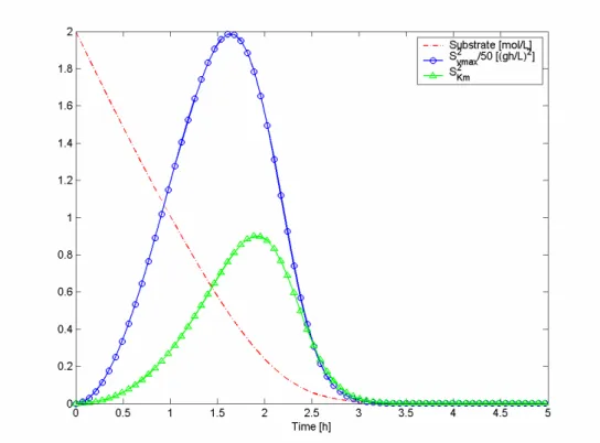
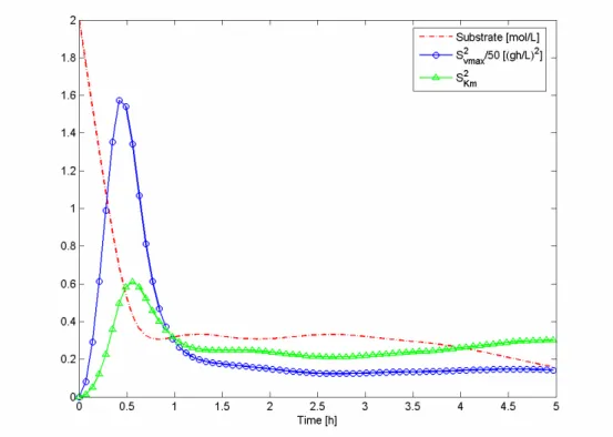
The substrate concentration as well as the squares of the sensitivities profile, for batch
process of criterion A using error 1, are presented in Figure 4.1. These profiles
Figure 4.1: Substrate concentration and squared sensitivities of the batch process using criterion A and
error 1, for experimental design
The FIM is influenced by values of the sensitivities at sampling time and, therefore, to
obtain the best values of FIM, these time points must be optimized. The sensitivity with
respect to vmax is always higher than Km’s, which means that the estimation error of vmax
will be lower than the one of Km’s. If the squares of the sensitivities are divided one by
the other, for example
( )
( )
iK i v
t S
t S
m 2 2
max
, it will be possible to know that vmax will be determined
with more precision at high concentrations of substrate, while Km will have a more
accurate value at low substrate concentration, because the previous quotient decreases
with the decrease of concentration (Figure 4.2). Consequently, the biggest difference is
obtained in the beginning which proves that vmax will be determined with higher
precision in higher substrate concentration and Km in lower concentration ranges, but
Figure 4.2: Quotient between Sv2
( )
timax and SKm
( )
ti 2and profile of substrate concentration through time
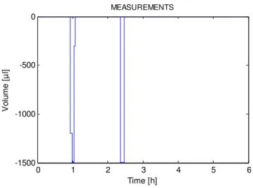
After the optimization was performed, 2 measurement points were obtained for every
criterion and every measurement error, confirming what had already been stated in
previous investigations that, for each parameter to be optimized, one measurement point
is obtained [6].
For the absolute constant error ( 1), the first measurement point is obtained around 0.95
h and the second at 2.33 h, except for criterion D for the first time tag, which is obtained
at 1.18 h. For every criterion, 5 replicates for each time of measurement were obtained.
For the linear growing measurement error ( 2), once again, criteria A and E had similar
results, having its measurement times around 1.26 h and 2.49 h with 5 replicates each.
CRLB’s are around 6.34 % and 23.4 % (for vmax and Km, respectively) for criteria A and
E. For criterion D, its CRLB’s are slightly larger with 6.82 % and 25.6 %, for vmax and
Km, respectively. Again, it is evident that according to what was mentioned before, the
vmax parameter is obtained with higher precision, since its Cramér-Rao lower bounds are
lower than those of Km. These results are presented on Table 4.1 and Table 4.2. The
results presented for E-mod criterion will not be analysed, since its CRLB values are
approximately two orders of magnitude larger than every other criteria, making them
not comparable.
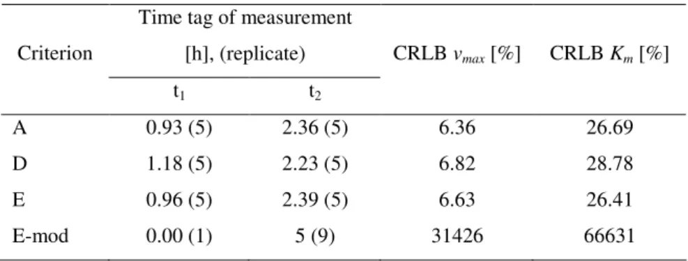
Table 4.1: Results of the optimization for batch process using the error 1
Time tag of measurement
[h], (replicate) Criterion
t1 t2
CRLB vmax [%] CRLB Km [%]
A 0.93 (5) 2.36 (5) 6.36 26.69
D 1.18 (5) 2.23 (5) 6.82 28.78
E 0.96 (5) 2.39 (5) 6.63 26.41
E-mod 0.00 (1) 5 (9) 31426 66631
Table 4.2: Results of the optimization for batch process using error 2
Time tag of measurement
[h], (replicate) Criterion
t1 t2
CRLB vmax [%] CRLB Km [%]
A 1.27 (5) 2.49 (5) 6.32 23.5
D 1.50 (5) 2.36 (5) 6.82 25.6
E 1.25 (5) 2.49 (5) 6.35 23.4
E-mod 0.00 (1) 5 (9) 19032 40167
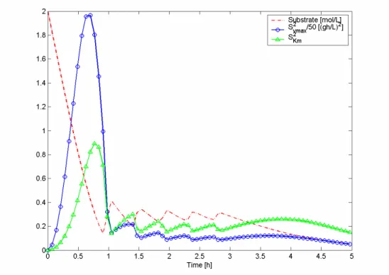
4.2. Experimental design for fed-batch (pulses) process
The concentration profile of an optimized fed-batch (pulses) process is shown in Figure
4.3 and the results of the optimal fed-batch (pulses) processes are presented in Table 4.3
and Table 4.4. While looking at the substrate concentration variation in time, it is clear
that in fed batch it lowers much quicker than the batch mode (concentration reaches
under 0.2 mol/L in about an hour while in batch process it takes approximately 2 hours)
consumed in the same period of time, either batch or fed-batch process, but the volume
is lower then, the concentration variation will be bigger. The initial concentration is the
maximum attainable (2 mol/L) and each pulse has a concentration of cpulse = 0.74 mol/L.
The volume of each pulse was 1.59 mL. These values are from the fed-batch (pulses)
process using 1 and criterion A.
Figure 4.3: Substrate concentration and squared sensitivities of the optimized fed-batch (pulses) process
using criterion A and error 1, for experimental design
Comparing the results to those of the batch process, some improvements are noticed in
error values of both parameters. CRLB for vmax lowered its value to around 5.58 % and
5.14 %, for 1 and 2, respectively, while CRLB for Km was improved to around 20.2 %
remainder replicates. Again, the existence of an early and a late measurements is clear,
as should be expected, so that there is one measurement with high and another with low
substrate concentration, making a good accuracy in parameters’ value possible.
For 2, the measurement time tags are slightly higher (around 0.19 h for the first and
0.37 h for the second, except for the D criterion which is lower – 3.43 h). For feeding
times, a slightly increase in times is detectable, about 0.15-0.30 h, except in the last two
feeding times in D criterion, which have the values 3.94 and 4.28 h. Comparing all
optimization criteria, one can see that the one that has the lowest overall CRLB is
A-criterion, with an average CRLB values of 6.34 % and 25.1 % for vmax and Km, using
batch process, while for fed-batch (pulses) process having as average CRLB’s 5.27 %
and 18.1 %, vmax and Km, respectively.
Table 4.3: Results of the optimization for fed-batch (pulses) process using the error 1
Time tag of feeding [h] Time tag of measurement
[h], (replicate) CRLB Criterion
t1 t2 T3 t4 t5
Feed volume (per
pulse) [mL]
t1 t2 vmax [%] Km [%]
A 0.95 1.41 1.85 2.29 2.72 1.59 0.43 (3) 4.06 (7) 5.49 20.2
D 0.86 1.40 1.97 2.48 4.85 1.60 0.54 (4) 4.08 (6) 5.65 22.6
E 0.93 1.39 1.83 2.26 2.69 1.59 0.40 (3) 4.04 (7) 5.61 20.2
E-mod 2.88 3.77 4.97 5 5 5.53 0.01 (1) 5 (9) 403 606
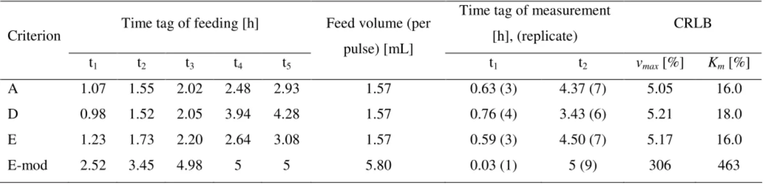
Table 4.4: Results of the optimization for fed-batch (pulses) process using the error 2
Time tag of feeding [h] Time tag of measurement
[h], (replicate) CRLB Criterion
t1 t2 t3 t4 t5
Feed volume (per
pulse) [mL]
t1 t2 vmax [%] Km [%]
A 1.07 1.55 2.02 2.48 2.93 1.57 0.63 (3) 4.37 (7) 5.05 16.0
D 0.98 1.52 2.05 3.94 4.28 1.57 0.76 (4) 3.43 (6) 5.21 18.0
E 1.23 1.73 2.20 2.64 3.08 1.57 0.59 (3) 4.50 (7) 5.17 16.0
E-mod 2.52 3.45 4.98 5 5 5.80 0.03 (1) 5 (9) 306 463
4.3. Experimental design for fed-batch (continuous) process
Figure 4.4 shows the substrate concentration profile for fed-batch (continuous) along
profile to the one of fed-batch (pulses), one can see that first one is “smoother”. This is
due to the fact that the feeding is not processed by pulses, which will make the
concentration change not as abruptly as in the discrete pulses mode.
When comparing the results with fed-batch (pulses), it is noticeable that the first set of
measurements moves towards earlier in time (higher substrate concentration), around
0.10 h for criteria A and E, for 1, and 0.18 h for 2; for criterion D, this change in time
is around 0.04 h for both measurement error types; the second set of measurements will
be performed later in time (lower substrate concentration), all of the measurements will
be performed at 5 h. Subsequently, both vmax and Km will be determined with a higher
accuracy.
Figure 4.4: Substrate concentration and squared sensitivities of the optimized fed-batch (continuous)
Table 4.5: Results of the optimization for fed-batch (continuous) process using the error 1
Time tag of measurement
[h], (replicate) CRLB Criterion
t1 t2 vmax [%] Km [%]
A 0.33 (3) 5 (7) 5.57 19.70
D 0.53 (4) 5 (6) 5.69 23.12
E 0.30 (3) 5 (7) 5.72 19.66
E-mod 0.06 (1) 5 (9) 89.7 139.4
Table 4.6: Results of the optimization for fed-batch (continuous) process using the error 2
Time tag of measurement
[h], (replicate) CRLB Criterion
t1 t2 vmax [%] Km [%]
A 0.46 (3) 5 (7) 5.32 15.93
D 0.72 (5) 5 (5) 5.44 20.06
E 0.40 (2) 5 (8) 5.75 15.43
E-mod 0.22 (1) 5 (9) 44.7 71.4
4.4. Equidistant sampling for batch and fed-batch (pulses) processes
When using the method of equidistant sampling, the purpose is to define upfront the
measurement and feeding times and see how good the parameters’ errors will be. When
observing the concentration profile, the influence of the feeding is not so noticeable like
in experimental design concentration profile and this is due to a slightly lower pulse
concentration, cpulse = 0.67 mol/L. This concentration is lower either because the mass
available for feeding is lower (5 mmol) and of higher pulses’ volume (1.5 mL each).
Checking the results, it is clear that both batch and fed-batch (pulses) processes have
worst CRLB than the experimental design. For batch, the errors obtained were about
11.0 % and 45.4 %, for vmax and Km, respectively, while for fed-batch (pulses) 8.56 %
and 26.5 %. One can clearly see that the fed-batch (pulses) process results are better (Km
has almost half the error than in batch mode), which means that feeding, instead of
having all the substrate at the beginning, is a better way to obtain more reliable values
Figure 4.5: Substrate concentration and squared sensitivities of the fed-batch (pulses) process using
criterion A and error 1 for equidistant sampling’ method
Table 4.7: Time tags for the equidistant sampling and its results
Time tag of feeding [h] Time tag of measurement [h] CRLB Criterion Error
Type t1 T2 t3 T4 t5 t1 t2 T3 t4 t5 t6 t7 t8 t9 t10 vmax, % Km, %
1 11.04 48.03
Batch
2
- - - 0.5 1.0 1.5 2.0 2.5 3.0 3.5 4.0 4.5 5.0
11.04 42.83
1 8.48 29.06
Fed-batch
2
0.83 1.67 2.50 3.33 4.17 0.5 1.0 1.5 2.0 2.5 3.0 3.5 4.0 4.5 5.0
8.64 23.89
4.5. Comparison between experimental design and equidistant measurement points for
experimental design, however, is not the best for every value, i.e., a lower
corresponding CRLB value might not be found for every value of vmax and Km. With the
data that is presented on those figures, one can also see which is the optimal parameter
value, i.e., which parameter value has the lowest CRLB.
For the first measurement error, the lowest CRLB with respect to vmax is around vmax =
0.124 mol/(g.h) for the three criteria and while the lowest CRLB with respect to Km is
around 0.338 mol/L for criteria A and E and 0.286 mol/L for criterion D. For these
parameters’ value the corresponding CRLB are 6.51 % and 27.0 %. For 2 the lowest
CRLB in respect to vmax value is around 0.124 mol/(g.h) and the lowest CRLB in respect
to Km is 0.314 mol/L for criteria A and E and 0.271 mol/L for criterion D.
The reason why the lowest CRLB values are not obtained with the values of the rough
estimates might be the fact that all optimization criteria (A, D and E) cover
experimental conditions for both parameters at the same time. Here, the change of one
parameter is considered by fixing the other one and, therefore, a smaller CRLB can
occur.
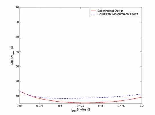
The range in which a smaller error for experimental design for parameter vmax is
observed is between 0.095 and 0.150 mol/(g.h), while for Km it is between 0.159 and
0.670 mol/L. For the second measurement error ( 2), the first range is almost the same,
Figure 4.6: CRLB vmax dependence on real values of vmax for experimental design (Km fixed to 0.3 mol/L)
and equidistant sampling using 1, for batch process
Figure 4.7: CRLB Km dependence on real values of Km for experimental design (vmax fixed to 0.12
mol/(g.h)) and equidistant sampling using 1, for batch process
Table 4.8: Lowest CRLB’s and its corresponding parameter for experimental design and range in which
experimental design is better than equidistant sampling for batch process using the error 1, for vmax
Experimental Design Range Criterion vmax with lowest CRLB [mol/(g.h)] Lowest CRLB vmax
Lower bound [mol/(g.h)] Higher bound [mol/(g.h)]
A 0.123 6.32 0.0937 0.149
D 0.126 6.64 0.0967 0.152
Table 4.9: Lowest CRLB’s and its corresponding parameter for experimental design and range in which
experimental design is better than equidistant sampling for batch process using the error 1, for Km
Experimental Design Range Criterion Km with lowest CRLB [mol/L] Lowest CRLB Km [%]
Lower bound [mol/L] Lower bound [mol/L]
A 0.342 26.3 0.161 0.719
D 0.286 28.6 0.150 0.595
E 0.335 26.1 0.165 0.696
Table 4.10: Lowest CRLB’s and its corresponding parameter for experimental design and range in which
experimental design is better than equidistant sampling for batch process using the error 2, for vmax
Experimental Design Range Criterion vmax with lowest CRLB [mol/(g.h)] Lowest CRLB vmax [%]
Lower bound [mol/(g.h)] Higher bound [mol/(g.h)]
A 0.123 6.28 0.0967 0.144
D 0.125 6.66 0.0997 0.146
E 0.124 6.28 0.0975 0.145
Table 4.11: Lowest CRLB’s and its corresponding parameter for experimental design and range in which
experimental design is better than equidistant sampling for batch process using the error 2, for Km
Experimental Design Range Criterion Km with lowest CRLB [mol/L] Lowest CRLB Km [%]
Lower bound [mol/L] Lower bound [mol/L]
A 0.316 23.3 0.180 0.606
D 0.271 25.2 0.154 0.508
E 0.312 23.4 0.176 0.602
For a judgement if experimental design procedure or equidistant sampling should be
carried out, a rough error is calculated as follows,
{
}
( )
% 100 Parameter
bound low -estimate Parameter
estimate, Parameter
-bound high min
×
This way it is possible to present a table that shows the maximum error that one
Table 4.12: Maximum parameter error for different criteria and measurement error type, for batch process
1 2
Criterion vmax [%] Km [%] vmax [%] Km [%]
A 21.9 46.2 19.4 40.0
D 19.4 50.0 16.9 48.7
E 20.6 45.0 18.8 41.2
Average 20.6 47.1 18.3 43.3
Having analysed all results of the comparison between the two approaches, for batch
process, it can be concluded that experimental design should be used instead of
equidistant sampling, if the parameter error is less than 19.5 % for vmax and less than
45% for Km (average percentages).
4.6. Comparison between experimental design and equidistant sampling for fed-batch
(pulses) process
The results for the fed-batch (pulses) process show a few changes when compared to the
batch process. The lowest CRLB parameter values almost present the same values as
the batch process but they are more scattered than the latter ones, having one of the
criteria values below the estimated value for vmax (criterion D, vmax =0.114 mol/(g.h) and
0.113 for each measurement error) and the other two above 0.12 mol/(g.h) (around
0.133 mol/(g.h) for the 1 and 0.130 mol/(g.h) for 2 for both criteria). For Km, its values are around 0.331 mol/L for the first measurement error and 0.302 mol/L for the second.
As for the error associated to the parameters’ value, one can see that for fed-batch
Figure 4.8: CRLB vmax dependence on real values of vmax for experimental design (Km fixed to 0.3 mol/L)
and equidistant sampling using 1, for fed-batch (pulses) process
Figure 4.9: CRLB Km dependence on real values of Km for experimental design (vmax fixed to 0.12
Table 4.13: Lowest CRLB’s and its corresponding parameter for experimental design and range in which
experimental design is better than equidistant sampling for fed-batch (pulses) process using the error 1,
for vmax
Experimental Design Range Criterion vmax with lowest CRLB [mol/(g.h)] Lowest CRLB vmax [%]
Lower bound [mol/(g.h)] Higher bound [mol/(g.h)]
A 0.131 5.41 0.0598 0.200
D 0.114 5.56 0.0500 0.173
E 0.136 5.44 0.0696 0.200
Table 4.14: Lowest CRLB’s and its corresponding parameter for experimental design and range in which
experimental design is better than equidistant sampling for fed-batch (pulses) process using the error 1,
for Km
Experimental Design Range Criterion Km with lowest CRLB [mol/L] Lowest CRLB Km [%]
Lower bound [mol/L] Higher bound [mol/L]
A 0.342 20.1 0.15 0.9
D 0.316 22.5 0.15 0.9
E 0.335 20.1 0.15 0.9
Table 4.15: Lowest CRLB’s and its corresponding parameter for experimental design and range in which
experimental design is better than equidistant sampling for fed-batch (pulses) process using the error 2,
for vmax
Experimental Design Range Criterion vmax with lowest CRLB [mol/(g.h)] Lowest CRLB vmax [%]
Lower bound [mol/(g.h)] Higher bound [mol/(g.h)]
A 0.128 4.98 0.0651 0.177
D 0.113 5.12 0.0500 0.154
A 0.301 16.0 0.15 0.9
D 0.305 18.0 0.15 0.9
E 0.301 16.0 0.15 0.9
As had previously been done before, for batch process, it is possible to calculate the
maximum parameter error that is possible to have (to perform experimental design
instead of equidistant sampling), being those errors presented on Table 4.17.
Table 4.17: Maximum parameter error for different criteria and measurement error type, for fed-batch
(pulses) process
1 2
Criterion
vmax [%] Km [%] vmax [%] Km [%]
A 50.2 50.0 45.8 50.0
D 44.1 50.0 28.4 50.0
E 42.0 50.0 42.6 50.0
Average 45.4 50.0 38.9 50.0
For fed-batch (pulses) process, one can say that knowing vmax and Km with a maximum
error of 42 % and 50 % (average values), respectively, one should opt by the approach
of experimental design.
5. Conclusion
From the results obtained in this study, it can be concluded that experimental design is,
in general, significantly better than equidistant sampling, when the final goal is the
identification of Michaelis-Menten kinetic parameters. The following more specific
conclusions can be taken from this study:
• In batch operation, the CRLB were reduced to about 40.2 % for vmax and 34.8 %
for Km when comparing experimental design and equidistant sampling;
• For fed-batch (pulses) the CRLB were reduced to about 41.6 % and 23.7 % for
vmax and Km when comparing experimental design and equidistant sampling
respectively. Thus, the improvement in Km is slightly lower than in the batch
case;
• Comparing between batch and fed-batch (pulses) allows to conclude that the
equidistant sampling (the error is reduced 15.4 % for vmax and 23.9 % for Km,
while in equidistant sampling it is reduced in about 22.5 % and 41.7
respectively);
• When employing experimental design, it is interesting to notice that from batch
to fed-batch (pulses), timestamps of the measurements move towards higher (the
first measurement) and lower (the second measurement) substrate concentration,
resulting in higher accuracy of the parameter’s estimates;
• Moreover, when comparing fed-batch (pulses) and fed-batch (continuous), one
can conclude that fed-batch (continuous) tends to lead to more accurate
parameter values, since the measurements are slightly closer to the beginning
and end time, in respect to first and second measurements, of the experiment;
• When comparing CRLB values between fed-batch (pulses) and fed-batch
(continuous), it is shown that they are very similar, having a difference of less
than 0.50 %;
• Comparing again both methods of experimental planning for a wide range of
vmax and Km parameter values, it is clear that the equidistant sampling is only
better in a very narrow region;
• Generally, timestamps for sampling and feeding of criteria A and E are similar.
The difference between these timestamps is generally under 2 %. These two
criteria also proved to be better than D-criterion in all situations, thus, it can be
concluded that for this kind of theoretical approach for determination of
parameters one should use either criterion A or E.
This experimental planning method can be applied to other types of biochemical
systems, by changing the kinetics’ expressions, which can be easily done by program
Another possible improvement would be to create a contour that shows how CRLB
values change with simultaneous changes in Michaelis-Menten parameters (vmax and
Km).
7. References
[1] Lindner, P.F.O., Hitzmann, B., 2006, “Experimental design for optimal
parameter estimation of an enzyme kinetic process based on the analysis of the
Fisher information matrix”, Journal of Theoretical Biology 238, 111-123.
[2] Faller, D., et al., 2003, “Simulation methods for optimal experimental design in
systems biology”, Simulation, Vol. 79, No.12, 717-725.
[3] Rodriguez-Fernandez, M., et al., 2006, “A hybrid approach for efficient and
robust parameter estimation in biochemical pathways”, BioSystems 83,
248-265.
[4] Holland, J.H., 1992. “Genetic algorithms”, Sci. Am. 267 (1), 66–72.
[5] Garcia, S., 1999, “Experimental design optimization and thermophysical
parameter estimation of composite materials using genetic algorithms”, PhD
Dissertation.
[6] Bezeau, M., Endrenyi, L., 1986, “Design of experiments for the precise
estimation of dose-response parameters: the Hill equation”, Journal of
Theoretical Biology, 123, 415-430.
[7] Murphy, E.F., et al., 2002, “Effective experimental design: enzyme kinetics in
the bioinformatics era”, Drug Discovery Today 7 (Suppl.), 187–191.
[8] Wager, T.D., Nichols, T.E., 2003, “Optimization of experimental design in
fMRI: a general framework using genetic algorithm”, Neuroimage 18, 293-309.
[9] Xiao, Z., Vien, A., 2003, “Experimental designs for precise parameter
8. Appendix A: Experimental design and equidistant sampling results
In this section, all results obtained for experimental design and equidistant sampling
0 1 2 3 4 5 6 -1
-0.5 0 0.5 1
FEED
Time [h]
V
o
lu
m
e
[
m
l]
0 1 2 3 4 5 6
-1500 -1000 -500 0
MEASUREMENTS
Time [h]
V
o
lu
m
e
[
µ
l]
0 1 2 3 4 5 6
0 5 10 15 20
S
0(t=0): 10 mmol, Sic(t=0): 2 mol/L, Vic(t=0): 5 mL
Time [h]
0 1 2 3 4 5 6
0 0.5 1 1.5 2
CRLBvmax+CRLBKm: 33.0501, CRLB
v max: 6.36318, CRLBKm: 26.6869
Time [h] Batch A-Criterion σ1
S*10 [mol/L] E [g/L] V [mL]
Substrate
S vmax
2 /50
S Km 2
0 1 2 3 4 5 6 -1
-0.5 0 0.5 1
FEED
Time [h]
V
o
lu
m
e
[
m
l]
0 1 2 3 4 5 6
-1500 -1000 -500 0
MEASUREMENTS
Time [h]
V
o
lu
m
e
[
µ
l]
15 20
S
0(t=0): 10 mmol, Sic(t=0): 2 mol/L, Vic(t=0): 5 mL
1.5 2
CRLBvmax+CRLBKm: 29.7806, CRLB
v max: 6.32313, CRLBKm: 23.4574 Batch A-Criterion σ2
Substrate
S vmax 2 /50
S Km 2 S*10 [mol/L]
0 1 2 3 4 5 6 -1
-0.5 0 0.5 1
FEED
Time [h]
V
o
lu
m
e
[
m
l]
0 1 2 3 4 5 6
-1500 -1000 -500 0
MEASUREMENTS
Time [h]
V
o
lu
m
e
[
µ
l]
0 1 2 3 4 5 6
0 5 10 15 20
S
0(t=0): 10 mmol, Sic(t=0): 2 mol/L, Vic(t=0): 5 mL
Time [h]
0 1 2 3 4 5 6
0 0.5 1 1.5 2
detFIM: 3.31897e+007, CRLB
v max: 6.81677, CRLBKm: 28.7823
Time [h] Batch D-Criterion σ1
Substrate
S vmax 2 /50
S Km 2 S*10 [mol/L]
E [g/L] V [mL]
0 1 2 3 4 5 6 -1
-0.5 0 0.5 1
FEED
Time [h]
V
o
lu
m
e
[
m
l]
0 1 2 3 4 5 6
-1500 -1000 -500 0
MEASUREMENTS
Time [h]
V
o
lu
m
e
[
µ
l]
10 15 20
S
0(t=0): 10 mmol, Sic(t=0): 2 mol/L, Vic(t=0): 5 mL
1 1.5 2
detFIM: 5.24544e+007, CRLB
v max: 6.82081, CRLBKm: 25.5823 S*10 [mol/L]
E [g/L] V [mL]
Substrate
Svmax2 /50
0 1 2 3 4 5 6 -1
-0.5 0 0.5 1
FEED
Time [h]
V
o
lu
m
e
[
m
l]
0 1 2 3 4 5 6
-2000 -1500 -1000 -500 0
MEASUREMENTS
Time [h]
V
o
lu
m
e
[
µ
l]
0 1 2 3 4 5 6
0 5 10 15 20
S
0(t=0): 10 mmol, Sic(t=0): 2 mol/L, Vic(t=0): 5 mL
Time [h]
0 1 2 3 4 5 6
0 0.5 1 1.5 2
λ
min: 157.917, CRLBv max: 6.63484, CRLBKm: 26.4057
Time [h] S*10 [mol/L]
E [g/L] V [mL]
Substrate
S vmax 2 /50
S Km 2 Batch E-Criterion σ1
0 1 2 3 4 5 6 -1
-0.5 0 0.5 1
FEED
Time [h]
V
o
lu
m
e
[
m
l]
0 1 2 3 4 5 6
-1500 -1000 -500 0
MEASUREMENTS
Time [h]
V
o
lu
m
e
[
µ
l]
10 15 20
S
0(t=0): 10 mmol, Sic(t=0): 2 mol/L, Vic(t=0): 5 mL
1 1.5 2
λ
min: 199.966, CRLBv max: 6.34902, CRLBKm: 23.4469 S*10 [mol/L]
E [g/L] V [mL]
Substrate
Svmax2 /50
0 1 2 3 4 5 6 -1 -0.5 0 0.5 1 V o lu m e [ µ l] FEED Time [h]
0 1 2 3 4 5 6
-3000 -2500 -2000 -1500 -1000 -500 0 MEASUREMENTS Time [h] V o lu m e [ µ l]
0 1 2 3 4 5 6
0 5 10 15 20 S
0(t=0): 10 mmol, Sic(t=0): 2 mol/L, Vic(t=0): 5 mL
Time [h]
0 1 2 3 4 5 6
0 0.5 1 1.5 2 λ
max/λmin: 92.3396, CRLBv max: 31426.2, CRLBKm: 66631
Time [h] S*10 [mol/L]
E [g/L] V [mL]
Substrate S vmax 2 /50 S Km 2 Experimental Design Batch Emod-Criterion σ1
0 1 2 3 4 5 6 -1
-0.5 0 0.5 1
V
o
lu
m
e
[
µ
l]
FEED
Time [h]
0 1 2 3 4 5 6
-3000 -2500 -2000 -1500 -1000 -500 0
MEASUREMENTS
Time [h]
V
o
lu
m
e
[
µ
l]
10 15 20
S
0(t=0): 10 mmol, Sic(t=0): 2 m ol/L, Vic(t=0): 5 mL
1 1.5 2
λmax/λmin: 92.3358, CRLB
v max: 19032.6, CRLBKm: 40166.8 Experimental Design Batch Emod-Criterion σ2
Substrate
Svmax2 /50
SKm2 S*10 [mol/L]
0 1 2 3 4 5 6 0 0.2 0.4 0.6 0.8 1 1.2 1.4 1.6 FEED Time [h] V o lu m e [ m l]
0 1 2 3 4 5 6
-2500 -2000 -1500 -1000 -500 0 MEASUREMENTS Time [h] V o lu m e [ µ l]
0 1 2 3 4 5 6
0 5 10 15 20 25
S0(t=0): 4.10657 mmol, Sic(t=0): 2 mol/L, Vic(t=0): 2.05329 mL
Time [h]
0 1 2 3 4 5 6
0 0.5 1 1.5 2
CRLBvmax+CRLBKm: 25.7175, CRLBv max: 5.49132, CRLBKm: 20.2262
Time [h] S*10 [mol/L]
E [g/L] V [mL]
Substrate S vmax 2 /50 S Km 2 Experimental Design Fed-Batch C-Criterion σ
1
0 1 2 3 4 5 6 0
0.5 1 1.5 2
FEED
Time [h]
V
o
lu
m
e
[
m
l]
0 1 2 3 4 5 6
-2500 -2000 -1500 -1000 -500 0
MEASUREMENTS
Time [h]
V
o
lu
m
e
[
µ
l]
15 20 25
S
0(t=0): 4.31222 mmol, Sic(t=0): 2 mol/L, Vic(t=0): 2.15611 mL
1.5 2
CRLBvmax+CRLBKm: 21.0039, CRLB
v max: 5.05259, CRLBKm: 15.9513
S*10 [mol/L] E [g/L] V [mL]
Substrate
Svmax2 /50
0 1 2 3 4 5 6 0
0.2 0.4 0.6 0.8 1 1.2 1.4 1.6
FEED
Time [h]
V
o
lu
m
e
[
m
l]
0 1 2 3 4 5 6
-2000 -1500 -1000 -500 0
MEASUREMENTS
Time [h]
V
o
lu
m
e
[
µ
l]
0 1 2 3 4 5 6
0 5 10 15 20 25
S
0(t=0): 4.02557 mmol, Sic(t=0): 2 mol/L, Vic(t=0): 2.01278 mL
Time [h]
0 1 2 3 4 5 6
0 0.5 1 1.5 2
detFIM: 3.63893e+007, CRLB
v max: 5.66165, CRLBKm: 22.6484
Time [h] S*10 [mol/L]
E [g/L] V [mL]
Substrate
Svmax2 /50
SKm2 Experimental Design Fed-Batch D-Criterion σ1
0 1 2 3 4 5 6 0
0.2 0.4 0.6 0.8 1 1.2 1.4 1.6
FEED
Time [h]
V
o
lu
m
e
[
m
l]
0 1 2 3 4 5 6
-2000 -1500 -1000 -500 0
MEASUREMENTS
Time [h]
V
o
lu
m
e
[
µ
l]
15 20 25
S
0(t=0): 4.324 mmol, Sic(t=0): 2 mol/L, Vic(t=0): 2.162 mL
1.5 2
detFIM: 7.44883e+007, CRLB
v max: 5.21362, CRLBKm: 17.9783
S*10 [mol/L] E [g/L] V [mL]
Substrate
S vmax 2 /50