Bank efficiency, market concentration and economic growth in the European Union

(1)

Carlos Pestana Barros & Nicolas Peypoch

A Comparative Analysis of Productivity Change in Italian and Portuguese Airports

WP 006/2007/DE _________________________________________________________

Cândida Ferreira

Bank efficiency, market concentration and economic

growth in the European Union

WP 38/2012/DE/UECE _________________________________________________________

De p a rtm e nt o f Ec o no m ic s

W

ORKING

P

APERS

ISSN Nº 0874-4548

School of Economics and Management

(2)

Bank efficiency, market concentration and economic growth in the European

Union

Cândida Ferreira [1]

Abstract

Well-functioning financial markets and banking institutions are usually considered to be a condition favourable to economic growth. The importance of bank efficiency and bank market concentration has also been the object of discussion, with the general belief that while they are of particular relevance in the context of the European Union, there is no consensus on their specific roles.

This paper aims to study the effects on economic growth of the efficiency of the banking institutions, measured through Data Envelopment Analysis (DEA), and also of the concentration of the bank markets, measured by the percentage share of the total assets held by the three largest banking institutions (C3) and the Herfindahl-Hirschman Index (HHI). Considering a panel of all 27 EU countries for the time period between 1996 and 2008, the study analyses the influence of these bank and market conditions not only on the Gross Domestic Product (GDP) but also on its components: the final consumption expenditure, the gross fixed capital formation, the export of goods and services and the import of goods and services.

The main findings point to the generally positive influence of bank cost efficiency on economic growth. More precisely, this influence is statistically significant for GDP and particularly with respect to the gross fixed capital formation. With regard to the bank market concentration, a generally negative influence is revealed, not only on GDP, but also on its components and is statistically more significant for the gross fixed capital formation, as well as for the export and import of goods and services.

Keywords: Bank efficiency, market concentration, economic growth, European Union. JEL Classification: G21; F43; D4; L11

[1]

ISEG-UTL – School of Economics and Management of the Technical University of Lisbon and UECE – Research Unit on Complexity and Economics

Rua Miguel Lupi, 20, 1249-078 - LISBON, PORTUGAL tel: +351 21 392 58 00

(3)

2

Bank efficiency, market concentration and economic growth in the European

Union

1. Introduction

Recently, the extent to which well-developed and accessible credit markets and institutions may be an important condition to economic growth has become clearer. Banks and other financial institutions are supposed to guarantee the financing of productive investments and activities, as they mobilise and allocate financial resources and also by means of their specific money-creation processes through bank credit. At the same time, well-functioning markets and financial institutions may decrease the transaction costs and asymmetric information problems. In addition, they are supposed to play an important role in identifying investment opportunities, selecting the most profitable projects, mobilising savings, facilitating trading and the diversification of risk, as well as improving corporate governance mechanisms.

There is a large strand of literature that analyses theoretically and empirically the link between economic growth and the development of the financial systems (represented among many others, by such authors as King and Levine (1993), Levine and Zervos (1998), Guiso et. al. (2004) and Hassan et al. (2011). On the other hand, the study of the importance of bank efficiency and bank market concentration has also been the object of discussion and it is generally accepted that they are of particular relevance in the context of the European Union, although their roles still remain controversial (see Goddard et al., 2007; Molyneux, 2009; among others).

(4)

3 financing; furthermore, we have in mind the mechanisms through which savings are channelled to productive investments that contribute to economic growth. These mechanisms involve both financial intermediaries (mostly banking institutions, for indirect financing) and financial markets (for the direct financing). Thus, we analyse the importance to economic growth of the performance of the banking institutions (particularly of bank efficiency) and of market conditions (more precisely, of the market concentration).

In this context, our study contributes to the literature mostly in the following ways.

First, like Cetorelli and Gambera (2001), we test the importance to economic growth of the concentration of bank markets, here measured by the percentage share of the total assets held by the three largest banking institutions (C3) and the Herfindahl-Hirschman Index (HHI). However, in contrast to these authors (and among others, Rajan and Zingales, 1998; Claessens and Laeven, 2005; Maudos and Fernandez de Guevara, 2009), we do not consider the influence of the external financial dependence, but instead we analyse the effect of the efficiency of the banking institutions, measured through Data Envelopment Analysis (DEA).

Second, we analyse the influence of these bank and market conditions not only on the Gross Domestic Product (GDP), but also on its components: final consumption expenditure, gross fixed capital formation, the export of goods and services and the import of goods and services.

Third, we consider a panel of all 27 EU member states for a relatively long time period: between 1996 and 2008. By the middle of the 1990s, Europe was preparing for the implementation of the single currency and many of the actual member states were adapting to new market conditions, whereas 2008 may be considered to mark the onset of the current financial crisis. We will not analyse the consequences of this crisis, but rather the situation during the 12 years preceding it, and in all 27 current members of the European Union.

(5)

4 fixed capital formation. In relation to the bank market concentration, our results are in line with those obtained by, for instance, Cetorelli and Gambera (2001), as concentration has a general negative influence not only on GDP, but also on its components and is statistically more significant for the gross fixed capital formation and also for the export and import of goods and services.

The remainder of the paper is organised as follows: Section 2 presents a brief literature review; Section 3 explains the methodological framework and the data used; Section 4 reports the main results of our estimations; and Section 5 concludes.

2. Brief literature review

During recent decades, and particularly since the renowned King and Levine (1993) paper, there has been an increase of empirical studies at the aggregate level which explain output variables with financial ratios and variables such as liquid liabilities, bank loans to the private sector, or stock market capitalisation, which may be representative of the development of the financial systems and institutions.

In one such study, Levine and Zervos (1998), using data for 49 countries for the period 1976-1990, conclude that there is a strong correlation between the rates of real per-capita output growth and stock market liquidity.

(6)

5 A few years later, Beck et al. (2004) used the ratio of the value of credit from financial intermediaries to the private sector, divided by GDP as a proxy to capture the depth and breadth of the financial intermediation in a panel of 52 countries over the period 1960 to 1999. They conclude that financial development is not only clearly pro-growth but also pro-poor, that is, in countries with better-developed financial intermediation, income inequality declines more rapidly.

Analysing these studies, we agree with Khan and Senhadji (2000), who, in providing a review of the literature and empirical evidence of the relationship between financial development and economic growth, concluded that the results of these studies indicate that while the general effects of financial development on the outputs are positive, the size of these effects varies with the different variables considered, with the indicators of financial development and with the estimation method, data frequency or the defined functional form of the relationship.

Furthermore, Rajan and Zingales (1998) argued that there is no clear causality between financial development and economic growth and proposed further tests to analyse the mechanism through which financial development may promote economic growth taking into account both country and sectoral effects. Rather than adhering to the traditional explanation of economic growth by proxies of the financial development, Rajan and Zingales (1998) test the hypothesis that financial markets and banking institutions not only reduce the cost of financing, but also help to combat the problems provoked by asymmetrical information, assuming in their test that the sectors most dependent on external financing will be the ones that grow faster and in line with the development of the financial markets and institutions to which these sectors have access.

(7)

6 Until the 1990s, there was a general belief that mergers did not clearly contribute to bank performance improvements and several empirical findings were consistent with the traditional structure conduct performance statements, in particular with the “quiet life hypothesis” (e.g. Berger and Hannan, 1989, 1998; Hannan and Berger, 1991; Houston and Ryngaert, 1994; Pilloff, 1996).

From the year 2000, this general consensus was broken when particular attention was paid to such specific characteristics of the banking markets as the presence of asymmetric information, contagion phenomena and imperfect competition, or the specific impacts of bank concentration, competition and regulation on bank performance (among others, De Brand and Davis, 2000; Bikker and Haaf, 2002; Berger et al., 2004; Hasan et al., 2009; Schaeck et al., 2009).

With regard to the empirical tests of the relationship between the bank market structure (represented by the market share or concentration indices) and bank efficiency (measured either by parametric methods, like the Stochastic Frontier Analysis, or by non-parametric methods, like the Data Envelopment Analysis), several papers tend to support the efficient structure hypothesis, underlining the importance of the relationship between bank cost efficiency and bank concentration or market share (for instance, Goldberg and Rai, 1996; Punt and Van Rooij, 2003; Maudos and Fernandez de Guevara, 2007).

However, it is generally recognised that not many works have addressed the possible relationship between banking market structure, bank performance (particularly bank efficiency) and economic growth.

(8)

7 Comparing the financial systems of different countries and regions, Allen and Gale (2001) conclude that there is inherent inefficiency within the monopolistic power of banks, which may also adopt an excessively conservative approach while the competitive nature of markets tends to encourage innovation and growth-enhancing activities.

At the same time, and following Rajan and Zangales’ (1998) contribution, there is a stand of empirical studies that use industry-level and firm-level data to analyse the channels through which financial development contributes to economic growth.

In one such study, Cetorelli and Gambera (2001) develop the Rajan and Zangales (1998) model and, considering a sample of 41 countries and 36 economic sectors, for the time period 1980-1990, conclude that there is empirical evidence of a general depressing effect on growth associated with a concentrated banking industry, which impacts all sectors and all firms indiscriminately.

More recently, Maudos and Fernandez de Guevara (2009) used different measures of bank market competition for a sample of 21 countries and 53 economic sectors during the time period 1993-2003, concluding not only that there is a positive effect of financial development on the economic growth of the sectors most dependent on external finance, but also that the exercise of bank market power promotes economic growth.

(9)

8 At the same time, and specifically with regard to the measurement of the quality of the financial development and its possible influence on economic growth, Hasan et al. (2009) use a sample of 147 regions in 11 European countries, between 1996 ad 2004, finding that regional economic growth benefits significantly from more efficient banks.

3. Methodological framework and data used

We will take into account the model specification of Rajan and Zingales (1998) and the contributions of Claessens and Laeven (2004, 2005) to analyse the influence of market structure and banking competition on economic growth and the more recent contribution of Maudos and Fernandez de Guevara (2009), who used market concentration measures and banking competition measures to explain the growth of 53 economic sectors in 21 countries.

We will not consider the growth of economic sectors here, but rather we will test the influence of bank efficiency and bank market concentration on GDP growth and on its components: final consumption, investment, exports and imports.

The basic model to be estimated will be:

Growth i,t = α0 + α1 year dummiesi + α2 country dummiest + α3 lag1 growth i,t-1 + α4 bank

efficiency i,t + α5 bank market concentration i,t + α 6 control variables i,t (1)

Where:

Growth = natural logarithm of the GDP (at market prices), or of one of its components: final consumption, gross fixed capital formation, exports or imports;

i = EU country (1 = 1, ... 27); t = year (t = 1996, ..., 2008);

(10)

9 bank efficiency = natural logarithm of the Data Envelopment Analysis (DEA) bank cost efficiency;

bank market concentration = natural logarithm of the percentage share of the total assets held by the three largest banking institutions (C3) or natural logarithm of the Herfindahl-Hirschman Index (HHI);

control variables = return on assets (ROA) or return on equity (ROE).

The inclusion of the year and country dummies aims to capture the influence of the considered specific time period (between 1996 and 2008) and also the influence of the country-specific factors that affect the economic growth of the 27 EU member states.

In the next pages, before presenting the results of the estimated model, we need to present the explanatory variables of our model and particularly to specify how we measure bank efficiency and bank market concentration.

3.1. Bank efficiency

The research into efficiency is usually based on the estimation of efficiency frontiers with the best combinations of the different inputs and outputs of the production process and then on the analysis of the deviations from the frontier that correspond to the losses of efficiency.

Most of the empirical studies on the measurement of bank efficiency adopt either parametric methods, like the Stochastic Frontier Analysis (SFA), or non-parametric methods, in particular the Data Envelopment Analysis (DEA).

(11)

10 banks’ total costs will depend on three bank outputs: total loans, total securities and other earning assets; and also on three bank inputs: borrowed funds, physical capital and labour (see Appendix A for a presentation of the DEA methodology and the chosen bank outputs and inputs).

Our data are sourced from the IBCA-BankScope 2008 CD. The sample comprises annual data from consolidated accounts of the commercial and saving banks of all 27 EU countries between 1996 and 2008. Appendix B presents the annual number of banks for each country that are available in the BankScope CD and included in our sample.

Using the available data, the DEA frontier will be defined by the piecewise linear segments that represent the combinations of the best-practice observations, the measurement of efficiency being relative to the particular frontier obtained. If the actual production of one decision-making unit (DMU) lies on the frontier, this production unit will be considered perfectly efficient, whereas if it is situated below the frontier, the DMU will be inefficient; the distance of the actual to the potential level of production will define the level of efficiency of any individual DMU. Thus, with the DEA approach, the efficiency score for any DMU is not defined absolutely in comparison with a universal efficiency standard; rather, it is always defined as the distance to the particular production frontier, that is, in relation to the other DMUs that are included in the specific data set. As a consequence, DEA provides efficiency scores even in the presence of relatively few observations, which represents a great advantage in comparison with the parametric approaches (like the SFA), as the latter require the availability of sufficient observations to allow the estimation of specific production functions.

Appendix C reports the obtained DEA yearly bank cost efficiency results of the EU countries for the time period between 1996 and 2008.

(12)

11 and other, smaller countries including Belgium, Denmark, Finland, Luxembourg, Sweden and the Netherlands). On the other hand, for some of the new EU member states, there is a trend to the increase of bank cost efficiency (particularly evident for Bulgaria and Romania).

3.2. Bank market concentration

Among the possible concepts and measures of market concentration, we opt to use two of the most popular indicators: the percentage share of the total assets held by the three largest banking institutions (C3) of each EU member-state and the Herfindahl-Hirschman Index (HHI), which, also in terms of each member-state’s total bank assets, is calculated as the sum of the squares of the market shares of each of the country’s banking institutions.

For the interpretation of the HHI, we follow the general rule that considers the presence of low concentration if HHI <1000; if HHI > 1800, there is high concentration; and if 1000 < HHI < 1800, the market will be moderately concentrated.

To obtain the concentration measures C3 and HHI, we continue to use data sourced from the IBCA-BankScope 2008 CD: annual data from the consolidated accounts of the commercial and savings banks of all EU countries between 1996 and 2008.

The C3 and HHI results are presented in Appendix D and clearly show that, with some exceptions, there is a general increase in the bank market concentration. The exceptions are to be found in the Netherlands and Greece and most particularly in certain new EU member states, like Bulgaria, Romania and Poland, and also in the Czech Republic, Ireland, Latvia, Lithuania, Malta and Slovakia, although less strongly.

(13)

12 up to 2005), countries that clearly account for the majority of the banks included in our panel (see Appendix B).

3.3. Control variables

In our estimations, we will also consider the influence on economic growth (and on its main components) of two variables that are commonly used to analyse the performance of the banking sector: the return on assets (ROA) and the return on equity (ROE).

The ROA is the ratio of the net income to the total assets of the banks and is useful in the assessment of the use of the banks’ resources and their financial strength. However, for the banking industry, most analysts prefer to use the ROE, that is, the ratio of the net income to the banks’ equity, to judge the performance not only of an individual bank, but also of the entire bank sector.

The bank net income gives, by itself, a good idea of the bank’s performance, but it suffers from an important drawback: it does not take into account the bank’s size and it makes difficult the comparisons among different banking institutions and/or during different time periods. However, the use of the above-mentioned ratios corrects for the size of the banks and makes possible the comparisons among institutions for the same or for different time periods.

Thus, the ROA is a simple measure of bank profitability that gives a good idea of how well the bank administration is doing its job, that is, how well the bank’s assets are being used to generate profits. This is a clear bank performance measure, but not the most relevant for the bank’s shareholders. The bank’s shareholders are particularly interested in the relationship between the bank’s earning and their equity investment, which can be measured by the ROE.

(14)

13 Both ratios reveal the clear difficulties of the banking institutions of some important EU countries in 2008. With regard to the ROA, for the years before 2008, there are few negative results and only for some new EU member states and some critical years of Germany’s reunification process. Nevertheless, generally speaking, during the time period between 1996 and 2007, the ROA results obtained reveal a general tendency to the increase of the profits generated from the banks’ assets in most of the EU countries.

The ROE results confirm the negative situations in 2008 and the few negative values for the banking institutions of some new EU members and of the reunited Germany. However, for the years before 2008 there is no clear trend to the increase or decrease of the ROE results. On the contrary, the ROE results reveal clear oscillations in the ratio of the banks’ earnings and the equity investment of their shareholders in all EU countries.

3.4. Sources of data and series used

As was mentioned before, our sample includes yearly data from all 27 EU countries, for the time period between 1996 and 2008. All financial and bank performance variables are sourced from the IBCA-BankScope 2008 CD (annual data from the consolidated accounts of the commercial and saving banks, all in nominal values and in euros).

The macroeconomic data are sourced from the Eurostat statistical database and include: the Gross Domestic Product (GDP), the final consumption expenditure, the gross fixed capital formation, the exports of goods and services and also the imports of goods and services. All these series are at market prices (as are also the financial variables), in millions of ECUs up to 31.12.1998 and millions of euros from 1.1.1999.

(15)

14 pooled Dickey-Fuller test, or as an augmented Dickey-Fuller test, when lags are included and the null hypothesis is the existence of non-stationarity. This test is adequate for heterogeneous panels of moderate size, like the panels used in this paper, and it assumes that there is a common unit root process. The main results obtained are reported in Appendix F and clearly allow us to reject the existence of the null hypothesis, although for the macroeconomic variables, only of their first differences (and since these variables are expressed in logarithms, their differences can then be interpreted as growth rates).

Appendix G presents the summary statistics and the correlation matrix of the series of data used in the estimation of the equation (1).

4. Empirical results

The results of the estimation of equation (1) with robust OLS regressions are presented in Appendix H, where the different tables (from Table H1 to Table H5) report the results for the GDP and for its components. In all situations, four models are estimated, all including the first lag of the correspondent dependent variable, the year and the country dummies (whose specific results are not reported, but are available on request) and the constant; the four models differ by the combinations of the two measures of bank market concentration (HHI or C3) and the two control variables (ROA or ROE).

(16)

15 growth (natural logarithm). The same applies to the ROA and ROE ratios and they clearly contribute to the positive variation of the GDP growth. These results are in line with the empirical studies that conclude that financial development, or the good performance of the banking sector, facilitates economic growth (for example King and Levine, 1993; Levine and Zervos, 1998; Hassan et al., 2011).

Table 1 – Summary of the results obtained for GDP

Explanatory variables (model 1) Effect Explanatory variables (model 2) Effect

Lag1 GDP _-* Lag1 GDP _-*

DEA bank cost efficiency ₊** DEA bank cost efficiency ₊** Bank market concentration (HHI) measure _- Bank market concentration (C3) measure _- Return on assets (ROA) ratio ₊* Return on assets (ROA) ratio ₊*

Constant + * Constant + *

Lag1 GDP _-** Lag1 GDP _-**

DEA bank cost efficiency ₊* DEA bank cost efficiency ₊* Bank market concentration (HHI) measure _- Bank market concentration (C3) measure _- Return on equity (ROE) ratio + *** Return on equity (ROE) ratio + ***

Constant ₊* Constant ₊*

+ Positive effect; - negative effect. * Statistically significant at 10%; ** statistically significant at 5%; *** statistically significant at 1%.

Source: Estimation results of equation 1 reported in Table H1 of Appendix H.

Regarding the bank market concentration measures (the growth of the HHI and C3, measured by the respective natural logarithms), the results obtained, although statistically less strong, reveal their negative influence on the differences of the GDP growth. A similar conclusion was previously obtained by Centorelli and Gamberra (2001) who, using information on 41 countries and 36 manufacturing sectors in the 1980s, found a negative general effect of market concentration on economic growth for all sectors and firms.

(17)

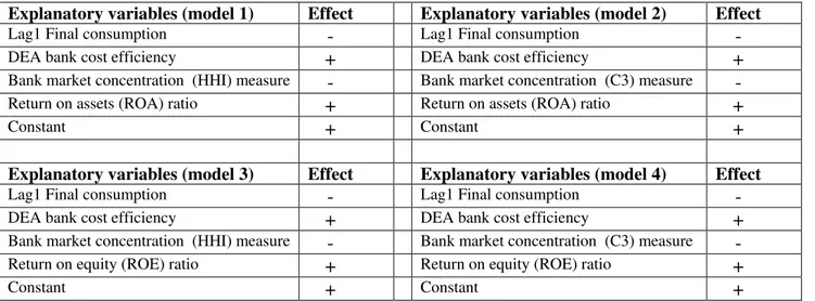
16 results are completely in line with those obtained for GDP, revealing that the variation of the growth of the final consumption expenditure represents an important part of the aggregate GDP, whereas consumption has its own specific dynamics and is less dependent on the evolution of the explanatory financial variables than GDP.

Table 2 – Summary of the results obtained for final consumption expenditure

Lag1 Final consumption - Lag1 Final consumption - DEA bank cost efficiency ₊ DEA bank cost efficiency ₊ Bank market concentration (HHI) measure _- Bank market concentration (C3) measure _- Return on assets (ROA) ratio ₊ Return on assets (ROA) ratio ₊

Constant ₊ Constant ₊

Lag1 Final consumption _- Lag1 Final consumption _- DEA bank cost efficiency ₊ DEA bank cost efficiency ₊ Bank market concentration (HHI) measure _- Bank market concentration (C3) measure _- Return on equity (ROE) ratio ₊ Return on equity (ROE) ratio ₊

Constant + Constant +

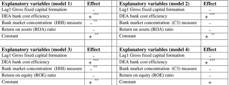
It is expected that well-functioning banking institutions play an important role not only in the saving mobilisation, but also in the diversification of risk, the identification of investment opportunities and the contribution to the gross fixed capital formation.

(18)

17 At the same time, and in line with the results already obtained for the GDP and the final consumption expenditure, the bank market concentration measures show a clear negative influence, particularly of the HHI, supporting the hypothesis that bank market concentration could be associated to less competition (defended, among others, by Bikker and Haaf, 2002 and Schaeck and Cihak, 2008) and also to lesser efforts in the selection of the most profitable projects.

Now, and contrary to our previous results for GDP and final consumption, the influences of ROA and ROE ratios are not only statistically irrelevant, but also negative. The explanation may be connected to the fact that the application of the financial resources in the gross fixed capital formation is an alternative to the other possible applications of these financial resources and also to the recognised increasing role of the non-traditional activities to explain the banking returns.

Table 3 – Summary of the results obtained for gross fixed capital formation

Lag1 Gross fixed capital formation _- Lag1 Gross fixed capital formation -DEA bank cost efficiency ₊*** DEA bank cost efficiency ₊*** Bank market concentration (HHI) measure _-** Bank market concentration (C3) measure _- Return on assets (ROA) ratio _- Return on assets (ROA) ratio _-

Constant + ** Constant + **

Lag1 Gross fixed capital formation _- Lag1 Gross fixed capital formation -DEA bank cost efficiency ₊*** DEA bank cost efficiency ₊*** Bank market concentration (HHI) measure _-** Bank market concentration (C3) measure _- Return on equity (ROE) ratio - Return on equity (ROE) ratio -

Constant ₊** Constant ₊

(19)

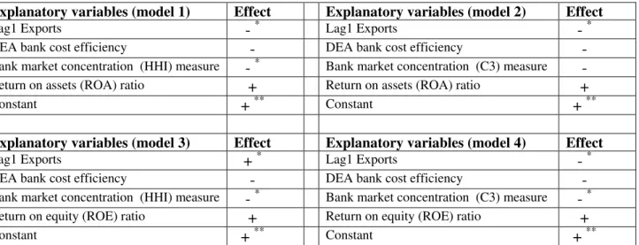
18 With reference to the influence of our explanatory variables, in general, they are not statistically significant, although their influences are in line with the results obtained for GDP (with the exception of the DEA cost efficiency, although this is clearly statistically not significant). However, in three of the considered models, the growth of bank market concentration, particularly when it is measured through the HHI, clearly has a negative influence on the growth rate of the exports of goods and services.

Table 4 – Summary of the results obtained for exports of goods and services

Lag1 Exports _-* Lag1 Exports _-* DEA bank cost efficiency _- DEA bank cost efficiency _- Bank market concentration (HHI) measure _-* Bank market concentration (C3) measure _- Return on assets (ROA) ratio + Return on assets (ROA) ratio +

Constant ₊** Constant ₊**

Lag1 Exports ₊* Lag1 Exports _-* DEA bank cost efficiency _- DEA bank cost efficiency _- Bank market concentration (HHI) measure - * Bank market concentration (C3) measure - * Return on equity (ROE) ratio ₊ Return on equity (ROE) ratio ₊

Constant + ** Constant + **

(20)

19 of the imports of goods and services, and now this influence is clearly statistically significant, both for the HHI and C3 concentration measures.

Table 5 – Summary of the results obtained for imports of goods and services

Lag1 Imports - (*) Lag1 Imports - (**) DEA bank cost efficiency ₊ DEA bank cost efficiency ₊ Bank market concentration (HHI) measure - (**) Bank market concentration (C3) measure - (**) Return on assets (ROA) ratio _- Return on assets (ROA) ratio _-

Constant + (**) Constant + (**)

Lag1 Imports _-(**) Lag1 Imports _-(**) DEA bank cost efficiency + DEA bank cost efficiency + Bank market concentration (HHI) measure _-(**) Bank market concentration (C3) measure _-(*) Return on equity (ROE) ratio - Return on equity (ROE) ratio -

Constant ₊(**) Constant ₊(**)

5. Summary and conclusions

(21)

20 consumption expenditure, the gross fixed capital formation, goods and services exports and goods and services imports.

We consider a panel of all 27 EU member states for the time period between 1996 and 2008. The macroeconomic data are sourced from the Eurostat statistical database, and all financial and bank performance variables are sourced from the IBCA-BankScope 2008 CD, including the available annual data from consolidated accounts of the commercial and saving banks.

Our results confirm the assumption that well-functioning financial institutions will contribute positively to economic growth (empirically confirmed by the large strand of literature mostly following the pioneering contribution of King and Levine, 1993). During the considered 12 years, a period when all EU member states were preparing either for the new market conditions of the European Monetary Union, or to become a new EU member, or indeed to confront all of these changes and challenges, just before the current financial crisis, there is clear evidence of a generally positive influence of bank cost efficiency on economic growth. However, this influence is statistically more significant for GDP and particularly for the gross fixed capital formation. Regarding the bank market concentration, our results are in line with those obtained by Cetorelli and Gambera (2001), among others, since concentration has a generally negative influence on GDP and on its components, this influence being statistically more significant for the gross fixed capital formation, for the export and import of goods and services.

(22)

21 • In all models, the obtained F statistics and the relatively high (for panel data) R-squares

point to the validity of the estimation results for GDP. Furthermore, there is clear and statistically significant evidence of the positive influence of the growth of the DEA bank cost efficiency, as well as on the ROA and the ROE ratios on the GDP growth rate.

• For the final consumption expenditure, the obtained results, although completely in line with those obtained for GDP, are now statistically less relevant, revealing that the final consumption expenditure may be an important part of the GDP aggregate expenditure but the growth rate of the final consumption has its own dynamics and is less dependent on the market and bank cost efficiency conditions than the other components of GDP.

• With regard to the growth rate of the gross fixed capital formation, there is statistically strong evidence of the positive influence of the growth of the DEA bank cost efficiency, confirming the important role of well-functioning banking institutions in increasing the gross capital formation. Moreover, the negative effect of the bank market concentration growth is also clear and statistically highly significant when concentration is measured through the Helfindahl-Hirschman Index.

• The results obtained for the exports of goods and services, although mostly in line with those reported for GDP and final consumption, are now statistically less relevant, confirming that the exports growth rate mainly depends on its own dynamics and most particularly on “other factors”, like the decisions of the rest of the world.

(23)

22

References

Allen, F and D. Gale (2001) Comparing Financial Systems, Cambridge,MA: MIT Press.

Banker, R. D., A. Charnes, A. and W. W. Cooper (1984) “Some models for the estimating technical and scale inefficiency in Data Envelopment Analysis”, Management Science, 30, pp. 1078-1092.

Beck, T., A. Demirgüç-Kunt and R. Levine (2004) Finance, Inequality and Poverty: Cross-Country

Evidence, World Bank Policy Research Working Paper No.3338.

Berger, A. N. and T. H. Hannan (1989) “The Price-Concentration Relationship in Banking” Review of Economics and Statistics, 71, pp. 291–299.

Berger, A. N. and T. H. Hannan (1998) “The Efficiency Cost of Market Power in the Banking Industry: A Test of the ‘Quiet Life’ and Related Hypotheses” Review of Economics and Statistics, 80, pp. 454–465.

Berger, A.N., A., Demirgüç-Kunt, R. Levine and J. G. Haubrich (2004) “Bank Concentration and Competition: An Evolution in the Making”, Journal of Money, Credit and Banking, 36, pp. 433-453.

Bikker, J. and K. Haaf (2002) “Competition, concentration and their relationship: An empirical analysis of the banking industry”, Journal of Banking andFinance, 26, pp. 2191-2214.

Carbó Valverde, S., D.B. Humphrey and F. Rodriguez Fernández (2003) “Deregulation, bank Competition and Regional Growth”, Regional Studies, 37 (3), pp. 227-237.

Cetorelli, N. and M. Gambera (2001): “Banking market structure, financial dependence and growth: international evidence from industry data”, Journal of Finance, 56, pp. 617-648.

Charnes A., W.W. Cooper and E. Rhodes (1978) “Measuring the Efficiency of Decision-Making Units”, European Journal of Operational Research, 2, pp. 429 – 444.

Claessens, S. and L. Laeven (2004) “What drives bank competition? Some international evidence”,

Journal of Money, Credit, and Banking, 36, pp. 563-583.

Claessens, S. and L. Laeven (2005):“Financial dependence, banking sector competition, and economic growth”, Journal of the European Economic Association, 3 (1), pp. 179-207.

Coelli, T.J., D. S. Prasada Rao and G. Battese (1998) An Introduction to Efficiency and Productivity

Analysis, Norwell, Kluwer Academic Publishers.

De Bandt, O. and E.P. Davis (2000) “Competition, Contestability and Market Structure in European Banking Sectors on the Eve of EMU”, Journal of Banking and Finance,24, pp. 1045-1066.

Demirguç-Kunt, A. and R. Levine (1999) Bank-Based and Market-Based Financial Systems: Cross

Country Comparisons, World Bank Policy Research Working Paper, No 2143.

Goldberg, L., and A. Rai (1996) “The Structure-Performance Relationship in European Banking”

Journal of Banking and Finance, 20, pp-745-771.

Goddard, J.A., Molyneux, P., and Wilson, J. O. S. (2007) “European banking: an overview”, Journal

of Banking and Finance, 31, pp. 1911-1935.

Guiso, L., T. Jappelli, M. Padula, and M. Pagano, M. (2004) “Financial market integration and economic growth in the UE”, Economic Policy, 19, pp. 523-577

Hannan, T. H. and A. N. Berger (1991) “The Rigidity of Prices: Evidence from the Banking Industry.” American Economic Review , 81, pp. 938–945.

Hasan, I., M. Koetter and M. Wedow (2009) “Regional growth and finance in Europe: Is there a quality effect of bank efficiency?”, Journal of Banking and Finance,33, pp. 1446-1453.

(24)

23 Houston, J. F. and M. Ryngaert (1994) “The overall gains from large bank mergers”, Journal of

Banking and Finance,18, pp. 1155-1176.

Khan, M. S. and A. Senhadji (2000) "Financial Development and Economic Growth: An Overview" IMF Working Paper No 209.

King, R. and R. Levine (1993) “Finance and Growth: Schumpeter Might be Right”, Quarterly

Journal of Economics, 108 (3), pp. 717-737.

Levin, A, C. Lin and C. Chu (2002) “Unit Root Tests in Panel Data: Asymptotic and Finite Sample Properties”, Journal of Econometrics, 108, pp.1-24.

Levine, R. and S. Zervos (1998) “Stock markets, banks and economic growth”, American Economic Review, 88 (3), pp. 537-558.

Maudos, J. and J. Fernandez de Guevara (2007) “The Cost of Market Power in Banking: Social Welfare Loss vs. Cost Inefficiency”, Journal of Banking and Finance, 31, pp. 2103 -2125.

Maudos, J. and J. Fernandez de Guevara (2009) Banking competition, financial dependence and

economic growth, Munich Personal RePEc Archive, MPRA Paper No.15254.

Molyneux, P. (2009) “Do Mergers Improve Bank Productivity and Performance? in Productivity in

the Financial Services, Edited by M. Balling, E. Gnan, F. Lierman and J.-P. Schoder, SUERF Studies,

Vienna, pp. 23-43.

Pilloff, S. J. (1996) “Performance changes and shareholder wealth creation associated with mergers of publicly traded banking institutions”, Journal of Money, Credit and Banking, 28, pp.294-310.

Punt, L., and M. Van Rooij (2003) “The Profit-Structure Relationship and Mergers in the European Banking Industry: An Empirical Assessment”, Kredit und Kapital, 36, pp. 1-29.

Rajan, R. and L. Zingales (1998) “Financial dependence and growth”, AmericanEconomic Review 88, pp. 559-587.

Schaeck, K. and M. Cihak (2008) How does competition affect efficiency and soundness in banking?

New empirical evidence, ECB Working Paper Series, N. 932.

Shaeck, K., M. Cihak and S. Wolfe (2009) “Are more competitive banking systems more stable?”,

Journal of Money, Credit and Banking, 41, pp.711-734.

Thanassoulis, E. (2001) Introduction to the Theory and Application of Data Envelopment Analysis. A

Foundation Text with Integrated Software, USA, Kluwer Academic Publishers.

Thanassoulis, E., Portela M.C.S. and O. Despic (2007) “DEA – The Mathematical Programming Approach to Efficiency Analysis” in The Measurement of Productive Efficiency and Productivity

(25)

24

Appendix A - Data Envelopment Analysis (DEA)

DEA was originally presented in Charnes et al. (1978), assuming constant returns to scale, which can be accepted as optimal but only in the long run. Later, Banker et al. (1984) introduced an additional convexity constraint (λ) and allowed for variable returns to scale. Following also Coelli

et al. (1998), Thanassoulis (2001) and Thanassoulis et al. (2007), we can assume that at any time

t, there are N decision-making units (DMUs) that use a set of X inputs (X = x1, x2, ..., xk) to

produce a set of Y outputs (Y = y1, y2, ..., ym), thus obtaining the DEA input-oriented efficiency

measure of every i DMU, solving the following optimisation problem:

∑

= = = = ≥ ≤ ≥ N 1 r N 1 r t kr N 1 r t mr , 1 0 x y . . min t r t r t ki i t r t mi t r i x y t s λ λ θ λ λ θ λ θ

The DEA approach provides, for every i decision-making unit (DMU, here every country’s banking sector), a scalar efficiency score (θi ≤ 1). If θi = 1, the DMU lies on the efficient frontier

and will be considered an efficient unit. On the contrary, if θi < 1, the DMU lies below the

efficient frontier and will be considered an inefficient unit; moreover, (1- θi) will always be the

measure of its inefficiency.

In the present study, the data are sourced from the IBCA-BankScope 2008 CD and the sample comprises annual data from the consolidated accounts of the commercial and savings banks of all EU countries between 1996 and 2008.

For the DEA estimates, we define the outputs and the input prices of the cost function, using the following variables:

Outputs:

1. Total loans = natural logarithm of the loans

2. Total securities = natural logarithm of the total securities

3. Other earning assets= natural logarithm of the difference between the total earning assets and the total loans

Inputs:

1. Price of borrowed funds = natural logarithm of the ratio interest expenses over the sum of deposits

2. Price of physical capital = natural logarithm of the ratio non-interest expenses over fixed asset

(26)

25

Appendix B – Yearly number of banks by EU country

1996 1997 1998 1999 2000 2001 2002 2003 2004 2005 2006 2007 2008

Austria 72 122 124 124 129 140 142 146 154 153 162 162 147 Belgium 97 91 75 73 68 69 72 73 72 71 58 47 34 Bulgaria 16 19 22 21 25 27 28 29 30 30 29 22 21 Cyprus 17 23 25 21 23 23 24 18 17 16 11 11 9 Czech Rep. 28 28 25 25 27 28 27 26 31 27 25 25 20 Denmark 113 113 117 118 123 116 113 112 129 120 123 121 109 Estonia 16 18 8 8 10 10 11 11 12 11 11 12 10 Finland 11 12 12 12 14 13 12 14 19 16 11 11 12 France 345 323 312 306 308 305 295 283 292 283 256 237 204 Germany 827 830 818 791 771 737 708 682 675 677 685 675 593 Greece 29 35 33 30 26 26 31 34 55 35 33 30 29 Hungary 34 33 34 37 39 35 37 33 33 36 35 31 26 Ireland 34 36 40 40 42 44 46 47 63 51 50 47 40 Italy 200 219 219 228 216 229 232 240 363 304 226 222 199 Latvia 21 25 24 24 25 26 27 30 33 36 36 36 33 Lithuania 11 13 13 14 16 16 16 17 17 17 18 18 15 Luxembourg 122 123 117 123 112 100 96 92 93 91 92 105 80

Malta 9 9 10 8 10 9 9 14 16 17 18 17 14

Netherlands 64 58 57 55 50 55 61 60 77 58 57 54 41 Poland 47 51 47 49 50 45 48 52 73 56 45 43 37 Portugal 41 44 44 43 37 36 33 32 44 34 31 31 25 Romania 8 11 27 30 31 30 31 29 32 29 29 28 27 Slovakia 19 23 24 20 22 20 21 19 19 25 17 17 16 Slovenia 29 29 24 26 25 23 20 20 23 29 23 22 21 Spain 206 216 207 198 204 213 211 208 256 192 184 151 136 Sweden 16 15 17 21 22 104 103 103 101 103 99 92 78 UK 191 196 200 195 195 197 204 206 257 203 190 170 148

(27)

26

Appendix C – Yearly Data Envelopment Analysis (DEA) cost efficiency measures of the EU member states

1996 1997 1998 1999 2000 2001 2002 2003 2004 2005 2006 2007 2008

Austria 0.702 0.629 0.595 0.760 0.720 0.616 0.643 0.694 0.676 0.707 0.662 0.678 0.715 Belgium 0.950 0.887 0.903 0.983 0.826 0.911 0.793 0.958 0.594 0.819 0.672 0.463 0.478 Bulgaria 0.149 0.270 1.000 1.000 1.000 1.000 1.000 0.970 0.937 0.832 1.000 1.000 0.915 Cyprus 1.000 1.000 1.000 1.000 1.000 1.000 0.914 0.725 0.695 0.679 0.837 0.800 0.937 Czech Rep. 0.945 0.803 0.579 0.632 0.859 0.741 0.681 0.716 0.838 0.897 1.000 1.000 1.000 Denmark 0.926 0.853 0.830 0.785 0.668 0.525 0.607 0.776 0.780 0.734 0.928 0.722 0.536 Estonia 1.000 0.864 0.730 0.647 0.717 0.765 0.621 0.587 0.760 0.777 0.893 0.711 0.669 Finland 0.783 1.000 1.000 1.000 0.737 1.000 0.687 0.677 1.000 0.905 1.000 0.845 0.579 France 0.818 0.699 0.687 0.739 0.552 0.547 0.578 0.576 0.531 0.577 0.606 0.597 0.712 Germany 0.948 0.889 1.000 0.981 0.772 0.762 0.887 0.934 0.956 0.776 0.821 0.699 0.606 Greece 0.754 0.685 0.643 0.604 0.734 0.781 0.949 1.000 1.000 1.000 1.000 0.967 0.991 Hungary 0.334 0.298 0.365 0.367 0.539 0.504 0.402 0.485 0.434 0.433 0.523 0.500 0.495 Ireland 1.000 1.000 1.000 1.000 1.000 1.000 1.000 1.000 0.951 1.000 1.000 0.849 0.959 Italy 1.000 0.872 1.000 1.000 0.975 0.802 0.921 0.924 1.000 0.958 0.984 0.741 0.740 Latvia 1.000 1.000 0.990 1.000 1.000 0.947 0.885 0.910 0.991 0.827 0.839 0.721 0.729 Lithuania 1.000 1.000 1.000 1.000 1.000 1.000 1.000 1.000 1.000 1.000 1.000 0.900 0.778 Luxembourg 0.879 0.690 0.730 0.696 0.654 0.508 0.564 0.697 0.673 0.757 0.523 0.544 0.524 Malta 1.000 0.911 0.953 0.888 0.932 1.000 1.000 1.000 1.000 1.000 1.000 1.000 1.000 Netherlands 1.000 1.000 1.000 0.874 0.764 0.759 0.748 0.852 0.822 0.779 0.821 0.882 0.564 Poland 0.700 0.591 0.708 0.596 0.597 0.604 0.528 0.593 0.616 0.605 0.985 1.000 0.928 Portugal 0.894 0.808 0.836 1.000 0.824 0.638 0.538 0.438 0.512 0.562 0.641 0.599 0.584 Romania 0.612 0.596 1.000 1.000 1.000 1.000 1.000 1.000 0.986 0.925 0.886 0.998 0.855 Slovakia 1.000 0.823 0.596 0.613 0.639 0.658 0.715 0.753 0.833 0.839 0.953 0.902 1.000 Slovenia 0.803 0.732 0.712 0.868 0.856 0.842 0.675 0.620 0.585 0.808 0.855 0.873 0.809 Spain 1.000 1.000 1.000 1.000 1.000 0.997 1.000 1.000 1.000 1.000 1.000 1.000 1.000 Sweden 0.632 0.675 0.708 0.724 0.514 0.638 0.677 0.695 0.589 0.626 0.695 0.509 0.440 UK 1.000 1.000 1.000 1.000 1.000 1.000 1.000 1.000 1.000 1.000 1.000 1.000 1.000

This Appendix presents the cost efficiency results obtained with DEA, considering three outputs (total loans, total securities, and other earning assets) and three inputs (price of borrowed funds, price of physical capital and price of labour).

Appendix D – Concentration measures: C3 and Herfindahl-Hirschman Index (HHI)

C3

1996 1997 1998 1999 2000 2001 2002 2003 2004 2005 2006 2007 2008

(28)

27 Malta 91.28 91.48 90.80 96.41 89.93 92.27 91.18 80.82 79.05 78.00 68.85 81.26 80.51 Netherlands 72.29 78.75 81.86 81.28 80.50 81.86 85.40 78.45 65.99 73.22 80.55 71.67 64.27 Poland 47.46 39.18 39.03 39.15 33.09 36.22 33.49 30.49 20.03 31.27 30.79 33.42 28.4 Portugal 32.46 28.90 30.56 31.00 45.10 42.92 46.01 48.25 41.15 54.49 56.48 54.00 53.78 Romania 96.56 85.88 60.93 63.28 58.69 55.34 53.98 58.79 50.89 50.86 49.44 52.14 47.75 Slovakia 71.20 62.95 50.94 57.74 57.72 56.66 56.80 57.34 62.12 45.87 56.82 52.38 55.02 Slovenia 41.63 44.77 45.80 42.42 45.54 51.81 51.97 59.51 56.74 52.77 49.06 50.93 48.18 Spain 31.36 33.82 33.63 38.46 38.21 36.51 32.81 31.89 31.44 36.11 32.98 33.15 32.72 Sweden 43.01 47.21 46.17 46.31 47.48 47.18 49.58 48.51 56.27 58.03 57.67 56.75 54.78 UK 28.24 26.96 22.32 25.46 24.59 24.95 27.95 28.14 23.46 30.85 29.10 33.09 35.57

Herfindahl-Hirschman Index (HHI)

1996 1997 1998 1999 2000 2001 2002 2003 2004 2005 2006 2007 2008

Austria 913 1023 1281 1564 1622 1626 1419 1229 941 1221 1049 1311 1084

Belgium 758 733 1035 1659 1628 1900 1638 1336 1375 978 1445 1499 1499

Bulgaria 2487 1972 1395 1394 1242 1040 846 827 745 741 690 756 673

Cyprus 1799 1613 1560 1608 1356 1278 1315 1837 1899 2199 2719 2242 2308

Czech Rep. 1182 1160 1113 1289 1366 1321 1282 1296 935 1015 1018 1004 1004

Denmark 1209 1106 1106 1017 1268 1479 1519 1511 1194 1577 1542 1615 1570

Estonia 1014 997 2274 2411 2516 2867 2828 2849 3720 4025 4218 3378 3378

Finland 2237 2335 2375 2236 2386 3767 4311 2877 1947 2511 2758 2793 2857

France 420 455 472 595 581 601 513 537 519 586 626 649 682

Germany 283 262 344 355 385 376 320 341 336 390 392 535 624

Greece 1099 981 914 792 896 899 869 856 485 870 812 853 845

Hungary 806 869 665 643 589 645 660 796 835 821 885 857 798

Ireland 1375 1410 1071 1171 1172 1023 1129 1081 815 886 963 1006 1065

Italy 333 326 397 412 431 469 437 411 401 591 807 1051 1025

Latvia 907 822 1028 932 847 865 828 744 660 716 750 697 735

Lithuania 1368 1329 1500 1944 1823 1696 1613 1362 1265 1256 1174 1079 1057

Luxembourg 301 299 333 330 346 371 398 392 366 381 365 276 318

Malta 3731 3759 3699 4156 3578 3680 3706 2683 2437 2370 1938 2639 2606

Netherlands 2061 2541 2647 2569 2543 2581 3232 2620 1597 2110 2418 1895 1701

Poland 962 714 794 687 597 731 668 583 377 612 613 645 550

Portugal 663 584 624 629 1025 997 1103 1158 1036 1273 1393 1310 1327

Romania 4249 2626 1733 1582 1388 1324 1254 1408 1160 1150 1102 1103 972

Slovakia 2127 1766 1240 1486 1443 1308 1301 1330 1437 978 1306 1202 1253

Slovenia 927 1032 1043 901 1017 1195 1218 1338 1234 1080 1130 1195 1087

Spain 464 502 507 600 645 600 515 500 482 654 565 561 563

Sweden 1148 1255 1243 1239 1253 1225 1298 1281 1575 1632 1598 1605 1563

UK 502 493 423 463 466 480 514 517 397 542 529 612 654

This Appendix presents the obtained yearly EU countries’ concentration measures with the C3 (that is, the percentage share of the total assets held by the three largest banking institutions) and the

(29)

28

Appendix E – Return on assets (ROA) and return on equity (ROE)

ROA

1996 1997 1998 1999 2000 2001 2002 2003 2004 2005 2006 2007 2008

Austria 0.0026 0.00345 0.00286 0.00403 0.00419 0.00325 0.00252 0.00348 0.00375 0.00462 0.00902 0.00586 -0.00142

Belgium 0.00302 0.00302 0.00287 0.00468 0.0057 0.00555 0.00387 0.00456 0.00431 0.00461 0.00684 0.00334 -0.01741

Bulgaria 0.05388 0.0967 0.00694 0.01875 0.02756 0.0168 0.01766 0.02099 0.01911 0.02024 0.01917 0.02198 0.02267

Cyprus 0.00389 0.00377 0.00541 0.01176 0.01105 0.00705 -0.00211 -0.0002 0.00202 0.00476 0.00888 0.01536 0.0116

Czech Rep. 0.00324 -0.00751 -0.00996 -0.00912 0.00383 0.00149 0.01318 0.01391 0.01344 0.01442 0.01357 0.0137 0.01222

Denmark 0.00834 0.00804 0.0072 0.00615 0.00603 0.00511 0.00455 0.00656 0.00565 0.00669 0.00719 0.00557 -0.00063

Estonia 0.02395 0.02263 -0.01593 0.01879 0.0171 0.02385 0.02386 0.02296 0.02127 0.01772 0.01719 0.02002 0.01383

Finland 0.00365 0.00862 0.00448 0.00815 0.01414 0.01517 0.00474 0.01658 0.00773 0.00868 0.00884 0.00965 0.00502

France 0.00073 0.00165 0.00269 0.00314 0.00481 0.00388 0.00349 0.00386 0.00497 0.00443 0.00571 0.00282 -0.00105

Germany 0.00231 0.00222 0.00377 0.00219 0.00399 -0.00018 -0.0019 -0.00203 0.00051 0.00269 0.00359 0.00388 -0.00223

Greece 0.00559 0.00606 0.00721 0.02243 0.0131 0.00954 0.00489 0.00747 0.00536 0.00921 0.00834 0.01075 0.0043

Hungary 0.01177 0.01083 -0.00029 0.00374 0.0114 0.0136 0.01482 0.01735 0.02394 0.01839 0.01721 0.01623 0.01344

Ireland 0.00687 0.00695 0.00766 0.00733 0.006 0.00464 0.00439 0.00522 0.00548 0.00551 0.0063 0.00611 0.0008

Italy 0.00201 0.00071 0.00462 0.00634 0.00728 0.00536 0.00433 0.00505 0.00608 0.00727 0.00775 0.00641 0.00419

Latvia 0.03149 0.02642 -0.06331 0.00926 0.01632 0.01551 0.01397 0.01374 0.01609 0.01839 0.01712 0.01735 0.00019

Lithuania -0.00612 0.00592 0.01042 0.01309 0.00778 0.00381 0.00829 0.01133 0.00999 0.00874 0.01178 0.01446 0.00947

Luxembourg 0.00426 0.00419 0.00543 0.00405 0.00469 0.00505 0.00516 0.00544 0.00493 0.00574 0.00857 0.00627 0.00262

Malta 0.00857 0.00941 0.00772 0.00757 0.01091 0.00818 0.00659 0.00876 0.01008 0.01233 0.01164 0.00941 -0.00227

Netherlands 0.00689 0.00675 0.00682 0.0067 0.00834 0.00707 0.00453 0.0061 0.00509 0.00688 0.00686 0.00805 -0.00883

Poland 0.0217 0.01648 0.00751 0.0107 0.01053 0.00763 0.00429 0.00355 0.01339 0.01722 0.0171 0.01973 0.016

Portugal 0.00586 0.00756 0.0075 0.0079 0.00914 0.00725 0.00654 0.00683 0.00509 0.00652 0.00755 0.00721 0.00288

Romania 0.00241 0.00074 -0.009 0.02758 0.02114 0.02552 0.01705 0.01196 0.02172 0.01683 0.01594 0.0131 0.0202

Slovakia 0.00182 -0.00696 -0.02133 0.01443 0.0153 0.01043 0.01232 0.0131 0.01082 0.00999 0.01105 0.0115 0.00873

Slovenia 0.01058 0.00956 0.01151 0.00645 0.01095 0.00511 0.00706 0.00615 0.00767 0.0073 0.00899 0.00929 0.00439

Spain 0.00619 0.00698 0.00783 0.00803 0.00826 0.00808 0.00764 0.00773 0.00747 0.00773 0.0089 0.00978 0.0069

Sweden 0.00945 0.00487 0.00717 0.00674 0.00756 0.00888 0.0045 0.00582 0.00885 0.00683 0.00677 0.00658 0.00454

UK 0.00674 0.00597 0.00834 0.00793 0.00794 0.0071 0.00622 0.00761 0.00744 0.00537 0.00547 0.00592 -0.00009

ROE

1996 1997 1998 1999 2000 2001 2002 2003 2004 2005 2006 2007 2008

Austria 0.07012 0.08268 0.0717 0.10285 0.1149 0.08425 0.06325 0.07434 0.08538 0.09875 0.16321 0.09107 -0.02699

Belgium 0.10145 0.09688 0.08235 0.13048 0.1604 0.17411 0.10844 0.13201 0.13042 0.15421 0.21715 0.07971 -0.52826

Bulgaria 0.43574 0.64501 0.04117 0.10237 0.15356 0.11381 0.12309 0.14553 0.16157 0.17414 0.17626 0.19653 0.18565

Cyprus 0.06761 0.0682 0.0941 0.15086 0.11837 0.08053 -0.02424 -0.00296 0.03704 0.09008 0.11125 0.15764 0.13239

Czech Rep. 0.04608 -0.11873 -0.15207 -0.14085 0.05733 0.02374 0.18834 0.18377 0.16247 0.17876 0.17501 0.20417 0.14958

Denmark 0.13266 0.14013 0.12551 0.11145 0.11017 0.10189 0.09585 0.13581 0.12381 0.13881 0.13917 0.11885 -0.01584

Estonia 0.26234 0.25425 -0.10693 0.12701 0.12888 0.18962 0.18476 0.18313 0.20602 0.20292 0.22375 0.25453 0.14777

Finland 0.07584 0.1886 0.09463 0.16671 0.22149 0.23956 0.07312 0.17018 0.08563 0.1005 0.0965 0.13678 0.09833

France 0.02058 0.0491 0.07574 0.08075 0.12459 0.10213 0.08729 0.09581 0.13134 0.12659 0.15251 0.08743 -0.03695

Germany 0.0647 0.06262 0.10468 0.06207 0.10063 -0.00403 -0.0478 -0.05344 0.0154 0.07803 0.10829 0.11397 -0.07949

Greece 0.12395 0.12592 0.12222 0.21942 0.15107 0.12468 0.07597 0.11189 0.08771 0.13803 0.11176 0.1466 0.0771

Hungary 0.20067 0.14938 -0.00464 0.05168 0.14947 0.17457 0.17517 0.19713 0.2474 0.21231 0.189 0.18294 0.16369

Ireland 0.10778 0.11656 0.12663 0.12916 0.09938 0.09332 0.10073 0.13648 0.13956 0.1512 0.1691 0.16367 0.0252

Italy 0.03248 0.01212 0.07539 0.10621 0.12109 0.08584 0.06809 0.07376 0.09107 0.09731 0.11052 0.07958 0.05588

Latvia 0.2347 0.21165 -0.79227 0.09451 0.18878 0.16992 0.15678 0.15339 0.18947 0.22583 0.21638 0.20573 0.0024

Lithuania -0.0944 0.06697 0.08455 0.10784 0.06946 0.03556 0.07332 0.1123 0.11137 0.11295 0.16206 0.19346 0.11498

Luxembourg 0.13237 0.13567 0.15398 0.11146 0.12008 0.12174 0.11354 0.12027 0.10508 0.12224 0.17984 0.13193 0.05362

Malta 0.15712 0.16442 0.10927 0.10722 0.1479 0.1102 0.08934 0.05892 0.07043 0.09368 0.08918 0.08777 -0.02371

Netherlands 0.1077 0.11702 0.12257 0.13324 0.14828 0.13617 0.0971 0.13562 0.15143 0.16493 0.166 0.16065 -0.25869

Poland 0.24709 0.1869 0.08864 0.12328 0.11412 0.08001 0.04391 0.03965 0.12701 0.16575 0.16663 0.19204 0.17613

Portugal 0.09731 0.12965 0.11553 0.12514 0.16528 0.13154 0.10931 0.10743 0.08646 0.11704 0.11874 0.11894 0.05323

Romania 0.03886 0.00847 -0.07063 0.17422 0.12891 0.14468 0.10438 0.08074 0.1699 0.15345 0.16463 0.15455 0.22711

Slovakia 0.03798 -0.14916 -0.82112 0.23768 0.21061 0.13332 0.13958 0.14107 0.12162 0.12898 0.15206 0.15506 0.11975

Slovenia 0.09374 0.08089 0.11398 0.06774 0.11554 0.05954 0.08655 0.07417 0.09183 0.09395 0.11265 0.11967 0.05467

Spain 0.10724 0.1181 0.12561 0.12915 0.11746 0.1159 0.1095 0.11587 0.10342 0.11944 0.13925 0.15256 0.11552

Sweden 0.23566 0.12267 0.19192 0.16768 0.20256 0.22153 0.115 0.13852 0.20442 0.16303 0.16075 0.16533 0.1289

UK 0.14577 0.12942 0.16932 0.14853 0.14254 0.12455 0.11284 0.13373 0.15684 0.14866 0.15404 0.15892 -0.00381

(30)

29

Appendix F – Panel unit root tests

Levin, Lin and Chu (2002) (LEVINLIN) tests:

Variables coefficient t-star P > t

First difference of the natural logarithm of the GDP -0.91877 -12.12891 0.0000 First difference of the natural logarithm of the final consumption -0.89094 -11.08223 0.0000 First difference of the natural logarithm of the gross fixed capital formation -0.87761 -9.74921 0.0000 First difference of the natural logarithm of the exports -0.98552 -13.34454 0.0000 First difference of the natural logarithm of the imports -0.79163 -9.83498 0.0000 Natural logarithm of DEA bank cost efficiency -0.43473 -4.25875 0.0000 Natural logarithm of bank market concentration (C3) measure -0.25417 -5.02867 0.0000 Natural logarithm of bank market concentration (HHI) measure -0.28545 -6.12162 0.0000 Return on assets (ROA) ratio -0.80155 -9.52113 0.0000 Return on equity (ROE) ratio -0.70968 -6.57430 0.0000

Appendix G – Summary statistics and correlations of the used series

Summary statistics

Variables (*) Mean Stand. Dev. Min Max Observations

GDP

OVERALL .0730185 .0562873 -.1317225 .2970152 N =324 BETWEEN .0349147 .0210996 .1360545 i = 27

WITHIN .0446177 -.1524267 .2422771 T = 12

Final consumption

OVERALL .0705547 .0528931 -.1204023 .2857208 N =324

BETWEEN .0341886 .017408 .1296475 i = 27

WITHIN .0408487 -.1574834 .228831 T = 12

Gross fixed capital formation

WITHIN .0848381 -.2398363 .3632473 T = 12

Exports

WITHIN .0739588 -.1836856 .5052467 T = 12

Imports

WITHIN .0749834 -.1747626 .411267 T = 12

DEA bank cost efficiency

OVERALL -.2407343 .263962 -1.903809 0 N =351

BETWEEN .1907762 -.8439925 0 i = 27

WITHIN .1858178 -1.869049 .1695398 T = 13

C3 concentration measure

(31)

30 BETWEEN .3719245 2.949454 4.444684 i = 27

WITHIN .1618877 3.198322 4.393741 T = 13

HHI concentration measure

OVERALL 6.949937 .6210185 5.568116 8.368878 N =351 BETWEEN .5865469 5.836045 8.030219 i = 27

WITHIN .2311326 5.996883 8.00785 T = 13

ROA

WITHIN .0078239 -.0652238 .0771008 T = 13

ROE

OVERALL .1105632 .1080092 -.82112 .64501 N =351

BETWEEN .037707 .0404331 .2041869 i = 27

WITHIN .101454 -.7784199 .5513863 T = 13

Correlation matrix

Variables (*)

GDP Final

consumption

Gross fixed capital formation

Exports Imports DEA C3 HHI ROA ROE

GDP 1.000

Final

consumption 0.9457 1.000 Gross fixed

capital

formation 0.7499 0.6755 1.000

Exports 0.5782 0.4658 0.4050 1.000

Imports 0.6228 0.5533 0.6058 0.9023 1.000

DEA 0.1548 0.1500 0.2145 0.0143 0.0547 1.000

C3 0.0665 0.0933 -0.0096 -0.0211 -0.0530 0.0494 1.000

HHI 0.0702 0.0946 -0.0167 -0.0164 -0.0530 0.0336 0.9818 1.000

ROA 0.3276 0.2898 0.1314 0.2303 0.2338 -0.0443 0.0933 0.1175 1.000

ROE 0.2075 0.1449 0.0459 0.1419 0.1324 -0.0028 0.0023 0.0348 0.8064 1.000

(*) More precisely, the variables used are:

GDP = First difference of the natural logarithm of the Gross Domestic Product Final consumption = First difference of the natural logarithm of the final consumption

Gross fixed capital formation = First difference of the natural logarithm of the gross fixed capital formation Exports = First difference of the natural logarithm of the exports

Imports = First difference of the natural logarithm of the imports

DEA bank cost efficiency = Natural logarithm of the DEA (Data Envelopment Analysis) bank cost efficiency C3 concentration measure = Natural logarithm of the bank market concentration (C3) measure

HHI concentration measure = Natural logarithm of the bank market concentration (Herfindahl-Hirschman Index) measure ROA = Return on assets ratio

(32)

31

Appendix H – Estimation results of the model represented by the equation 1(*) for GDP and its components (**)

Table H1 – GDP

Estim. Coefiicient Standard Error t-statistic P-value Model 1

Lag1 GDP -.0071848 .003807 -1.89 0.060 DEA bank cost efficiency .0300956 .0148715 2.02 0.044 Bank market concentration (HHI) measure -.0143891 .0113649 -1.27 0.207 Return on assets (ROA) ratio .5765727 .2993796 1.93 0.055 Constant .136441 .0771146 1.77 0.078

F( 41, 281) = 13.53 Prob > F = 0.0000 R-squared = 0.51 Number of obs = 323

Model 2

Lag1 GDP -.0072858 .0038125 -1.91 0.057 DEA bank cost efficiency .030228 .0152627 1.98 0.049 Bank market concentration (C3) measure -.0186492 .0173772 -1.07 0.284 Return on assets (ROA) ratio .5573989 .3028159 1.84 0.067 Constant .1066834 .0638236 1.67 0.096

Model 3

Lag1 GDP -.0073208 .003697 -1.98 0.049 DEA bank cost efficiency .0249126 .0149545 1.67 0.097 Bank market concentration (HHI) measure -.0143963 .0112594 -1.28 0.202 Return on equity (ROE) ratio .0571032 .0216469 2.64 0.009

Constant .1335425 1.75 0.082

Model 4

Lag1 GDP -.0073991 .0036963 -2.00 0.046 DEA bank cost efficiency .0252481 .0151935 1.66 0.098 Bank market concentration (C3) measure -.018443 .0170693 -1.08 0.281 Return on equity (ROE) ratio .0558858 .021638 2.58 0.010 Constant .1030202 .0629114 1.64 0.103

F( 41, 281) = 13.05 Prob > F = 0.0000

(33)

32

Table H2 – Final consumption

Lag1 Final consumption -.0061036 .0039308 -1.55 0.122 DEA bank cost efficiency .0204266 .0147358 1.39 0.167 Bank market concentration (HHI) measure -.0087379 .0109251 -0.80 0.425 Return on assets (ROA) ratio 2645169 .310571 0.85 0.395 Constant .1056773 .0736742 1.43 0.153

F( 41, 281) = 11.91 Prob > F = 0.0000

R-squared = 0.48 Number of obs = 323

Model 2

Lag1 Final consumption -.0062289 .0039245 -1.59 0.114 DEA bank cost efficiency .0191408 .015116 1.27 0.206 Bank market concentration (C3) measure -.0156481 .0165433 -0.95 0.345 Return on assets (ROA) ratio .2463248 .3118491 0.79 0.430 Constant .1040328 .0598293 1.74 0.083

Model 3

Lag1 Final consumption -.0059839 .0038121 -1.57 0.118 DEA bank cost efficiency .0176473 .0147898 1.19 0.234 Bank market concentration (HHI) measure -.0086698 .0108329 -0.80 0.424 Return on equity (ROE) ratio .0346203 .0211535 1.64 0.103 Constant .103507 .0731082 1.42 0.158

F( 41, 281) = 11.94 Prob > F = 0.0000

Model 4

Lag1 Final consumption -.0060845 .0038017 -1.60 0.111 DEA bank cost efficiency .0166097 .0150126 1.11 0.270 Bank market concentration (C3) measure -.0151678 .0162347 -0.93 0.351 Return on equity (ROE) ratio .0335062 .0209705 1.60 0.111 Constant .1005776 .0588447 1.71 0.089

F( 41, 281) = 11.80 Prob > F = 0.0000

(34)

33

Table H3 – Gross fixed capital formation

Lag1 Gross fixed capital formation -.0086819 .0062959 -1.38 0.169 DEA bank cost efficiency .0805218 .0300559 2.68 0.008 Bank market concentration (HHI) measure -.0465085 .0233284 -1.99 0.047 Return on assets (ROA) ratio -1.398121 .9409315 -1.49 0.138 Constant .3462776 .1644267 2.11 0.036

Model 2

Lag1 Gross fixed capital formation -.008731 .0063164 -1.38 0.168 DEA bank cost efficiency .0850035 .0304422 2.79 0.006 Bank market concentration (C3) measure -.0472685 .0330015 -1.43 0.153 Return on assets (ROA) ratio -1.438665 .9446563 -1.52 0.129 Constant .3462776 .1644267 2.11 0.036

Model 3

Lag1 Gross fixed capital formation -.0071703 .0062881 -1.14 0.255 DEA bank cost efficiency .0907374 .0334168 2.72 0.007 Bank market concentration (HHI) measure -.0460204 .0235382 -1.96 0.052 Return on equity (ROE) ratio -.0933274 .0705539 -1.32 0.187 Constant .3480401 .1657073 2.10 0.037

F( 41, 281) = 5.96 Prob > F = 0.0000

Model 4

Lag1 Gross fixed capital formation -.0071577 .0063471 -1.13 0.260 DEA bank cost efficiency .0958274 .0341574 2.81 0.005 Bank market concentration (C3) measure -.0455535 .0334307 -1.36 0.174 Return on equity (ROE) ratio -.0958592 .0704921 -1.36 0.175 Constant .1994248 .129321 1.54 0.124