Deep Learning in Melanoma Detection

F

E

U

P

Deep Learning in Melanoma Detection

Bruno Alexandre Oliveira Dias

Mestrado Integrado em Engenharia Informática e Computação Supervisor: Luís Paulo Reis

Co-Supervisor: Alexandra Oliveira

Deep Learning in Melanoma Detection

Bruno Alexandre Oliveira Dias

Mestrado Integrado em Engenharia Informática e Computação

Approved in oral examination by the committee:

External Examiner: Prof. Feliz Gouveia Supervisor: Prof. Luís Paulo Reis July 22, 2020

Abstract

Skin cancer is the most common type of cancer, one of the deadliest diseases in the world. How-ever, if detected early, the patient’s prognosis is very promising and long term survival rates im-prove significantly.

Usual diagnostics start with a dermatologist doing a visual examination of a skin lesion that the patient has noticed. There are a few problems with this: 1) The patient needs to have a minimum amount of knowledge to know what to look for, as well as being aware of skin lesions throughout their body. 2) The manual interpretation is time-consuming and prone to human errors. The use of dermatoscopy by dermatologists helps reduce the amount of human errors but it’s often not enough.

On another level, recent studies show that applying Machine Learning algorithms to the detec-tion of melanomas can perform on-par and even better than trained dermatologists. Deep learning specifically is becoming more and more used in image classification. Convolutional neural net-works are designed specifically for image classification and have been boasting great results in this problem. The ImageNet dataset contains millions of images of thousands of different categories and has been used over the years to develop multiple CNNs with great performance.

Recent studies have been applying CNNs pre-trained on the ImageNet dataset to other image classification problems, including melanoma detection. Combining the feature detection learned by pre-trained CNNs and applying it to a different domain, in a process known as transfer learning, can be extremely useful when trying to classify images using deep learning with a small dataset.

The HAM10000 dataset includes 10015 images of skin lesions, mainly Nevi and Melanomas, and is the largest dataset of its nature publicly available. In this work we train deep learning models based on the VGG16, one of the most famous CNNs created with the ImageNet dataset, using the transfer learning techniques of feature extraction and fine tuning, achieving performance on par with trained dermatologists and even beating them. Further, we will show how different changes to deep learning models affect their performance.

Keywords: skin cancer, melanoma, early diagnosis, Machine Learning, transfer learning, convo-lutional neural networks, image classification

Resumo

O cancro da pele é um dos tipos mais comuns the cancro, umas das doenças mais letais em todo o mundo. No entanto, quando detetado cedo, o prognóstico do paciente apresenta-se bastante promissor e a taxa de sobrevivência a longo prazo melhora significativamente.

No geral, diagnósticos de cancro de pele começam com a examinação visual de uma lesão na pele que o paciente notou e quis examinar profissionalmente. Existem alguns problemas com isto: 1) O paciente necessita de um mínimo conhecimento do que está à procura e de estar ciente das lesões da pele que tem no seu corpo. 2) A interpretação manual consome bastante tempo e é propensa a erros humanos. O uso de dermatoscopia por dermatologistas ajuda a diminuir esses erros, mas muitas vezes não é suficiente.

Por outro lado, estudos recentes mostram que aplicar algoritmos de Machine Learning na deteção de melanomas consegue atingir performance ao mesmo nível ou ainda melhor do que dermatologistas profissionais. O Deep Learning em específico está a ser cada vez mais usado em classificação de imagens. Convolutional Neural Networks (CNN) são desenhadas especificamente para a classificação de imagens e têm mostrado ótimos resultados neste problema. O dataset ImageNet contém milhões de imagens de milhares de diferentes categorias e tem sido usado ao longo dos anos para criar várias CNNs com alta performance.

Trabalhos recentes têm aplicado CNNs pré-treinadas no ImageNet em outros problemas de classificação de imagens, incluindo a deteção de melanomas. Combinando a deteção automática de caraterísticas aprendida por uma CNN pré-treinada e aplicando-a a um domínio diferente, num processo conhecido como transfer learning, pode ser extremamente útil para a classificação de imagens usando deep learning com um dataset pequeno.

O dataset HAM10000 inclui 10015 imagens de lesões da pele, principalmente de nevos melanocíti-cos e de melanomas, e é o maior dataset desta natureza publicamente disponível. Neste projeto são treinados modelos de deep learning baseados no VGG16, uma das CNNs criadas com o Im-ageNet mais famosas, utilizando técnicas de feature extraction e fine tuning, atingindo resultados ao mesmo nível e até acima de dermatologistas profissionais. Para além disso, vamos também mostrar como diferentes mudanças a modelos de deep learning afetam a sua performance.

Palavras-chave: cancro da pele, melanoma, diagnóstico precoce, Machine Learning, transfer learning, convolutional neural networks, classificação de imagens

Acknowledgements

I would like to take this opportunity to thank my supervisor Luís Paulo Reis and especially my co-supervisor Alexandra Oliveira for the support during the development of this dissertation. Their help was very important in particular during the final stages of writing and during a change in the topic of the dissertation.

The greatest thank you goes to my family and especially my parents for their continued support over the years and for always putting education first in their list of priorities.

A final thank you goes to all the friends I’ve made over five years in Porto. All the experiences we’ve lived will forever be on my memory and I hope we all stay in touch.

Bruno Dias

“The greatest glory in living lies not in never falling, but in rising every time we fall.”

Nelson Mandela

Contents

2 State Of the Art 7 2.1 Machine Learning . . . 7 2.1.1 Decision Tree . . . 8 2.1.2 Random Forest . . . 9 2.1.3 k-Nearest Neighbor . . . 9 2.1.4 Support-Vector Machine (SVM) . . . 10 2.2 Deep Learning . . . 10

2.2.1 Concepts and Techniques . . . 12

2.2.2 Neural Networks . . . 12

2.3 Transfer Learning . . . 18

2.3.1 Feature Extraction . . . 20

2.3.2 Fine Tuning . . . 22

2.3.3 Training and Optimization . . . 22

2.4 Performance Metrics . . . 25

2.5 Datasets and related work . . . 27

3 Methodology 31 3.1 Setup . . . 31

3.2 Dataset preparation . . . 31

3.3 Data loading and augmentation . . . 32

3.4 Transfer Learning . . . 33 3.4.1 Feature Extraction . . . 34 3.4.2 Fine Tuning . . . 35 3.5 Changing weights . . . 36 4 Results 37 4.1 Feature Extraction . . . 37 4.2 Fine tuning . . . 39

4.2.1 Base model partially trainable . . . 39

4.2.2 Base model fully trainable . . . 43

4.3 Changing class weights . . . 46

x CONTENTS

5 Conclusions and future work 49

List of Figures

1.1 Human Skin Anatomy. Obtained from [32]. . . 2

1.2 Photos of two different appearances of basal cell carcinomas. Obtained from [41]. 3 1.3 Photos of two different appearances of squamous cell carcinomas. Obtained from [27]. . . 3

1.4 Examples of melanomas with characteristic asymmetry, border irregularity, color variation, and large diameter. Obtained from [35]. . . 4

1.5 Photos of three different appearances of melanocytic nevi. Obtained from [19]. . 5

2.1 Illustration of the general appearance of a simple decision tree. . . 9

2.2 Visualization of k-NN algorithm. In this example, if k is 3 (inner circle) the test sample (green circle) is classified as a red triangle since there are 2 red triangle and 3 blue squares. If k is 5 (outer, dotted circle) the test sample is classified as a blue square (3 blue squares vs 2 red triangles). Image obtained from [71]. . . 10

2.3 Illustration of multiple hyperplanes separating two data groups and the choice of an optimal hyperplane. Source: [39]. . . 11

2.4 Illustration of an artificial neural network. . . 13

2.5 Illustration of the dot product operation done in a convolution. . . 14

2.6 Illustration of a typical CNN. Obtained from [10]. . . 15

2.7 ConvNet configurations. Column D and E represent the VGG16 and VGG19 ar-chitectures, respectively. Obtained from [68]. . . 17

2.8 Visualization of VGG16’s architecture. Obtained from [23]. . . 18

2.9 ResNet architectures. Column with 50 layers represents the ResNet50. Obtained from [30]. . . 19

2.10 ResNet skip connection. Obtained from [30]. . . 19

2.11 Illustration of a general example of transfer learning. The left represents the pre-trained network which, without the classifier, gets used as a base on the network to the right, transferring the knowledge obtained initially. . . 21

2.12 Illustration of a general example of a feature extraction approach to transfer learning. 22 2.13 Illustration of a general example of a fine-tuning approach to transfer learning. . . 23

3.1 Compact visualization of the VGG16 model without top classification layers. . . 33

3.2 Compact visualization of the new model with new top classification layers added with traditional method (left) and newer method (right). . . 35

4.1 Plots of validation AUC in training of models with different FC layers . . . 37

4.2 Plots of validation loss in training of models with different FC layers . . . 38

4.3 Plots of ROC curve in the evaluation of models with different FC layers . . . 38

4.4 Plot of validation AUC in training of model with GAP layer and base model par-tially trainable. . . 40

xii LIST OF FIGURES

4.5 Plot of validation AUC in training of model with FC layers with 2048 nodes and base model partially trainable. . . 40 4.6 Plot of validation loss in training of model with GAP layer and base model

par-tially trainable. . . 41 4.7 Plot of validation loss in training of model with FC layers with 2048 nodes and

base model partially trainable. . . 41 4.8 Plot of ROC curve in the evaluation of model with GAP layer and base model

partially trainable. . . 42 4.9 Plot of ROC curve in the evaluation of model with FC layers with 2048 nodes and

base model partially trainable. . . 42 4.10 Plot of validation AUC in training of model with GAP layer and base model fully

trainable. . . 43 4.11 Plot of validation AUC in training of model with 2048 nodes FC layers and base

model fully trainable. . . 44 4.12 Plot of validation loss in training of model with GAP layer and base model fully

trainable. . . 44 4.13 Plot of validation loss in training of model with 2048 nodes FC layers and base

model fully trainable. . . 45 4.14 Plot of ROC curve in the evaluation of model with GAP layer and base model

fully trainable. . . 45 4.15 Plot of ROC curve in the evaluation of model with 2048 nodes FC layers and base

model fully trainable. . . 46 4.16 Plot of ROC curve in the evaluation of model with GAP layer and base model

fully trainable, with manually set class weights. . . 47 4.17 Plot of validation AUC in training of model with GAP layer and base model fully

trainable, with manually set class weights. . . 47 4.18 Plot of validation loss in training of model with GAP layer and base model fully

List of Tables

2.1 Confusion Matrix . . . 25

2.2 Melanoma classification scores using two publicly available datasets. Compiled information on PH2 dataset obtained from [4]. . . 29

3.1 Dataset layout . . . 32

3.2 Estimated class weights . . . 35

3.3 Manually changed class weights . . . 36

4.1 Confusion Matrix of model with FC layers with 512 nodes . . . 38

4.2 Confusion Matrix of model with FC layers with 1024 nodes . . . 39

4.3 Confusion Matrix of model with FC layers with 2048 nodes . . . 39

4.4 Confusion Matrix of model with GAP layer and base model partially trainable. . 40

4.5 Confusion Matrix of model with 2048 nodes FC layers and base model partially trainable. . . 41

4.6 Confusion Matrix of model with GAP layer and base model fully trainable. . . . 43

4.7 Confusion Matrix of model with 2048 nodes FC layers and base model fully train-able. . . 44

4.8 Confusion Matrix of model with GAP layer and base model fully trainable, with manually set class weights. . . 46

Abbreviations

ANN Artificial Neural Network AdaGrad Adaptive Gradient Algorithm Adam Adaptive moments

BCC Basal Cell Carcinoma

CNN Convolutional Neural Network CPU Central Processing Unit DL Deep Learning

DNN Deep Neural Network DT Decision Tree

FC Fully connected GAP Global Averaging Pool GPU Graphics Processing Unit ML Machine Learning MSE Mean Square Error

RMSProp Root Mean Square Propagation ReLU Rectified Linear Unit

ResNet Residual Network

SCC Squamous cell carcinoma SGD Stochastic Gradient Descent SOTA State of the Art

SVM Support-Vector Machine k-NN k-Nearest Neighbor

Chapter 1

Introduction

1.1

Context

Skin cancer is the most common type of cancer, one of the deadliest diseases in the world. If de-tected early, the patient’s prognosis is very promising and long-term survival rates can be improved significantly [36].

As technology progresses and its’ role in society becomes more and more important, its use in the population’s health and well-being becomes imperative. Our health is one of our most important assets. To help keep it, technology can be used to assist medical professionals in their jobs, helping them use their time more efficiently and effectively. In order to understand how technology can be of use, first we need to understand how skin cancer presents itself and how it is traditionally diagnosed.

1.2

Motivation

The human skin is the largest organ of the human body and covers its’ outer area, protecting it from microbes and the elements. The skin also helps regulate body temperature and permits the sensations of touch, heat, and cold [32].

According to Millington in the book Skin, the skin is composed of mainly three layers [50] (illustrated in figure1.1):

• The epidermis is the outermost layer. It provides a waterproof barrier and is responsible for the skin tone.

• The dermis is the layer beneath the epidermis and contains tough connective tissue, hair follicles and sweat glands.

• The hypodermis is a deeper subcutaneous tissue that is mainly made of fat and connective tissue.

As any living organ, the skin can be affected by lesions that have varying degrees of severity and different consequences. A skin lesion is a part of the skin that has an abnormal growth or

2 Introduction

Figure 1.1: Human Skin Anatomy. Obtained from [32].

appearance compared to the skin around it [33]. There are many different types of skin lesions, ranging from freckles or other benign conditions to more serious problems, such as skin cancers.

There are three main types of skin cancer: basal cell carcinomas, squamous cell carcinomas and melanomas [36]. Apart from those, melanocytic nevi present their own clinical interest as they have the possibility of evolving into melanomas, despite not being cancerous themselves [72]. Distinction between types of skin cancer is mainly done by assessing different shapes, colors or textures. The appearance of complications such as ulcerations and the location of lesion can also be used as differentiating factors.

Basal cell carcinoma (BCC)

Although there are many clinical presentations of BCC, the most common characteristic type is a raised, pearly bump which can be ulcerative or asymptomatic. Sometimes small blood vessels (telangiectatic vessels) can be seen on the tumor [36].

This cancer type appears mostly in sun-exposed skin of the head, neck, torso and shoulders. High-risk areas for tumor recurrence after initial treatment include the central face (e.g., perior-bital region, eyelids, nasolabial fold, or nose-cheek angle), postauricular region, pinna, ear canal, forehead, and scalp [36].

1.2 Motivation 3

(a) BCC as a shiny bump or nodule (b) BCC as an open sore that does not heal

Figure 1.2: Photos of two different appearances of basal cell carcinomas. Obtained from [41].

Squamous cell carcinoma (SCC)

SCCs tend to present as a red, scaling, thickened patch, open sores or wart-like skin on sun-exposed portions of the skin, such as the ears, lower lip, and dorsa of the hands. They are composed of keratinizing cells, some are firm hard nodules and dome shaped like keratoacanthomas, and ulceration and bleeding may occur. If left untreated, SCCs may develop into a large mass [36].

(a) SCC as a persistent, scaly red patch

(b) SCC as a wart-like growth that crusts and some-times bleeds

Figure 1.3: Photos of two different appearances of squamous cell carcinomas. Obtained from [27].

Melanoma

Melanoma is a type of cancer that begins in melanocytes (cells that make the pigment melanin). Although it is most common in the skin, it can also start in the eye, the intestines, or other areas of the body with pigmented tissues [37].

Melanomas are identified by mainly five characteristics. The mnemonic ‘ABCDE’ helps to remember to look for a lesion’s asymmetry, borders, color, diameter and evolution (illustrated in figure1.4):

4 Introduction

• Border: Borders are irregular, the edges are often ragged, notched, or blurred in outline. The pigment may spread into the surrounding skin.

• Color: More than one color, with darker or variable discoloration. Shades of black, brown, and tan may be present. Areas of white, gray, red, pink, or blue may also be seen.

• Diameter: Usually above 6mm.

• Evolution: The mole changed in the past weeks or months. Changes can be in size, shape, color or feel. [37]

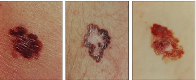
Figure 1.4: Examples of melanomas with characteristic asymmetry, border irregularity, color vari-ation, and large diameter. Obtained from [35].

Melanocytic Nevus

Commonly referred to as a mole, a melanocytic nevus is a type of melanocytic tumor that contains nevus cells [20]. They are commonly congenital or appear in childhood and teenage years [72].

Although typical moles consist of a simple brown spot, they can pose different characteristics: • Color and texture: Moles can be brown, tan, black, red, blue or pink. They can be smooth,

wrinkled, flat or raised. They may have hair growing from them. • Shape: Most moles are oval or round.

• Size: Usually smaller than 6mm, although congenital moles can be much bigger [72].

Melanocytic nevi are benign moles. Over time, however, these can change appearance and evolve into melanomas [72]. As about one third of melanomas derive from melanocytic nevi [17], it’s important to be able to distinguish the two, despite their similar appearance. The ideal scenario would be to reliably predict which nevi will evolve into melanoma and treat them before said evolution. Very often the patient is the one responsible for noting a lesion’s evolution and

1.3 Objectives 5

communicating it to a health professional, which makes it difficult for there to exist data recording the evolution of melanocytic nevi which could be used in an attempt to predict their evolution into melanomas [69]. Until standards change and historical data, containing different stages of nevi becoming melanoma, is recorded and made available, distinction between the two lesions is mostly done using symmetry, border irregularity and color characteristics.

(a) Small, brown and flat nevus (b) Dark, small and thick congeni-tal nevus

(c) Blue nevus

Figure 1.5: Photos of three different appearances of melanocytic nevi. Obtained from [19].

As the human population increases, there are more and more people recurring to hospitals and health clinics to see medical professionals.

Early diagnosis of certain conditions, such as some types of skin cancer, is mandatory as they can quickly become fatal. With the increase of the population, it can be difficult to have enough manpower to professionally and individually test every person regularly for signs of the early stages of skin cancer. Further, even professional dermatologists can’t diagnose these cancers with absolute certainty without recurring to invasive biopsies. Brinker [8] conducted a survey in which german dermatologists were asked to distinguish melanoma and nevi images out of different datasets of 100 dermoscopic or clinical images. This study shows a group of 157 dermatologists scoring an overall sensitivity of 74.1% and specificity of 60.0% using images obtained through dermoscopy tests and a group of 145 dermatologists scored an overall sensitivity of 89.4% and specificity of 64.4% using non-dermoscopic images.

Technology, specifically machine learning, can be helpful by providing reliable and accessible systems that are able to point the potential diagnostics, whether they will be used by the general population in self-examination or by dermatologists to help increase the reliability of diagnoses and hopefully reduce the need of recurring to biopsies when unnecessary.

1.3

Objectives

The objective of this dissertation is to create a machine learning system capable of classifying images as melanoma or melanocytic nevi with equal or higher scores than those achieved by dermatologists, while using the biggest publicly available skin lesion dataset, with reliable ground-truth labels, and comparing different approaches to image pre-processing, feature extraction and classification. Another objective is the analysis of the impact of changes to transfer learning classification models in a binary classification process.

6 Introduction

1.4

Document Structure

This document is structured in five chapters. After finishing this introduction, chapter two will focus on the state of the art, specifically of machine learning algorithms, deep learning and learning techniques, model performance metrics and a review of related work and datasets. Chapter three will hold a description of the methodology used in building and testing different methods. Chapter four will hold the results of relevant tests. Finally, chapter five will hold the conclusions and future work.

Chapter 2

State Of the Art

Several methods have been introduced to classify images and specifically melanoma. These meth-ods range from traditional machine learning algorithms such as k-Nearest Neighbors algorithms (k-NN) and linear support-vector machines (SVMs) to deep learning approaches using convolu-tional neural networks (CNNs).

This chapter will start by introducing the basics of machine learning and some of the traditional algorithms. This is followed by a description of artificial and convolutional neural networks and the use of transfer learning to quickly train new models based on pre - trained networks, using little amounts of data. After, we will introduce widely used performance metrics used to evaluate these algorithms. Finally, we will preview related datasets and works that share similarities with the proposed in this dissertation.

2.1

Machine Learning

Arthur Samuel defines Machine learning (ML) as the scientific study of algorithms and statistical models that computer systems use to perform a specific task without using explicit instructions, relying on patterns and inference instead [44].

Tom M. Mitchell provided a widely quoted, more formal definition of the algorithms studied in the machine learning field: "A computer program is said to learn from experience E with respect to some class of tasks T and performance measure P if its performance at tasks in T, as measured by P, improves with experience E" [52].

Machine Learning algorithms can be divided into three basic types, depending on the learning problem:

• Supervised learning is the task of learning a function that maps an input to an output based on example input-output pairs given. A number of N inputs is given to the algorithm where the output for each N input is known beforehand. A supervised learning algorithm analyzes the training data and produces an inferred function, which can be used for mapping new examples.

8 State Of the Art

• Unsupervised learning is a type of learning that helps find previously unknown patterns in a data set without pre-existing labels. A number of N inputs is given to the algorithm where the output for each N input is not known beforehand. This allows the modeling of probability densities functions of given inputs.

• Reinforcement learning is learning how to map situations to actions so as to maximize a numerical reward signal. The algorithm is not told which actions to take, but instead must discover which actions yield the most reward by trying them [73]. The algorithm is given a set of states about the environment and a set of actions, with an associated reward value, that can be taken to transition between states. With the given information, the algorithm must find the best actions to take for a specific environment.

Machine Learning algorithms can also be divided into three categories, depending on the out-put:

• Classification algorithms want to predict the class label output of an input (e.g. predicting if e-mails are spam or not).

• Regression algorithms want to predict a continuous quantity output of an input (e.g. pre-dicting houses’ selling price).

• Clustering algorithms group data according to their degree of similarity.

There are multiple machine learning algorithms already developed that can be used for various specific tasks. Despite not being originally designed with image classification in mind, some of these algorithms can be adapted to classify images, especially when using a different algorithm to automate feature extraction. Decision trees, random forests, k nearest neighbor and support-vector machines are some of the algorithms that can be used in this scenario.

These algorithms are still sometimes used in image classification but have been falling out of favour with the rise in interest of deep learning (a subset of machine learning) algorithms, par-ticularly convolutional neural networks, which are specifically designed for image classification. Deep learning concepts are later expanded in section2.2.

2.1.1 Decision Tree

Decision Tree (DT) is a supervised learning algorithm that can be used to solve both classification and regression problems. It takes the form of a tree structure with decision nodes and leaf nodes. A decision node has two or more branches. Leaf node represents a class label in the case of classification problems or a continuous value (typically a real number) in the case of regression problems. There are multiple algorithms that implement decision trees already developed and are widely used, such as ID3, C4.5 and CART (Classification and Regression Trees).

The Iterative Dichotomiser 3 (ID3) algorithm is mostly used for classification problems with discrete data and uses a top-down greedy approach to build a decision tree starting at the top and always choosing the best feature at the moment. The C4.5 algorithm is an extension to ID3 by the

2.1 Machine Learning 9

same author and shows some improvements such as the handling of both discrete and continuous data and pruning trees after creation by removing branches that don’t contribute significantly to the decision process. The CART algorithm can handle both classification and regression problems and uses a new metric named gini impurity 2.1, which measures how often a randomly chosen element from the set would be incorrectly labeled if it was randomly labeled, to create decision points for classification tasks [5,57,58,67].

Gini= 1 −

N

∑

i=1

p2_i (2.1)

Figure 2.1: Illustration of the general appearance of a simple decision tree.

2.1.2 Random Forest

A random forest is a supervised learning method that can be used for classification or regres-sion problems. In essence it consists of an ensemble of a multitude of different deciregres-sion trees where each individual tree predicts a class and the most common prediction is chosen as correct. Rather than having a single very complex tree, which tends to overfit, this algorithm uses multiple different trees, each sensitive to different feature dimensions [31].

Deep forest, or gcForest, is an ensemble of random forests in a cascading structure which is said to enable gcForest to do feature extraction in a similar way to deep neural networks [78].

2.1.3 k-Nearest Neighbor

The k-nearest neighbors algorithm (k-NN) is a non-parametric method used to solve both clas-sification and regression problems [2]. In both cases, the input consists of the k closest training examples in the feature space. The output depends on whether k-NN is used for classification or regression:

• Classification: the output is a class membership. An object is classified by a plurality vote of its neighbors, with the object being assigned to the class most common among its k

10 State Of the Art

nearest neighbors (k is a positive integer, typically small). If k = 1, then the object is simply assigned to the class of that single nearest neighbor.

• Regression: the output is the property value for the object. This value is the average of the values of k nearest neighbors.

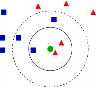
Figure 2.2: Visualization of k-NN algorithm. In this example, if k is 3 (inner circle) the test sample (green circle) is classified as a red triangle since there are 2 red triangle and 3 blue squares. If k is 5 (outer, dotted circle) the test sample is classified as a blue square (3 blue squares vs 2 red triangles). Image obtained from [71].

2.1.4 Support-Vector Machine (SVM)

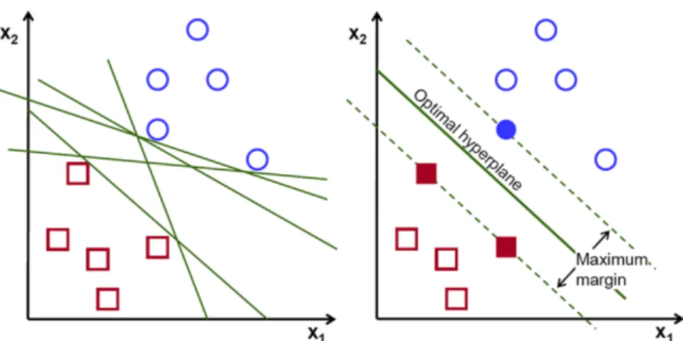
A support-vector machine is a supervised machine learning model that uses classification algo-rithms for two-group classification problems. In general, a SVM maps input vectors non-linearly to a very high-dimension feature space, where a linear decision surface, or hyperplane, is con-structed [16]. As seen in figure2.3, multiple hyperplanes can separate the data and, intuitively, the best hyperplane is the one where the distance from it to the nearest data point on each side is maximized. In general, to the increase in the margin between the hyperplane and nearest data points corresponds a decrease in the generalization error of the classifier [29].

2.2

Deep Learning

The concept of Deep Learning can be traced back to 1943 and the creation of a computer model based on the neural networks of the human brain by Walter Pitts and Warren McCulloch. In their seminal work "A Logical Calculus of Ideas Immanent in Nervous Activity” [48], they proposed a combination of algorithms and mathematics they called “threshold logic” with the aim of mim-icking human thought process. Having evolved over the years, their model remains a standard in current days.

2.2 Deep Learning 11

Figure 2.3: Illustration of multiple hyperplanes separating two data groups and the choice of an optimal hyperplane. Source: [39].

In 1958, Frank Rosenblatt published "The perceptron: a probabilistic model for information storage and organization in the brain" [62] introducing the percepton, capable of automatically learning a mapping from real-valued inputs to a binary output. Having only a single layer, per-ceptrons are only capable of learning linearly separable patterns. In 1969 Marvin Minsky and Seymour Papert published the famous book "Perceptrons" [51], which showed that networks of perceptrons were incapable of learning the XOR operation, a non-linear function.

Over the years deep learning kept slowly evolving. In 1965 the first working deep learning networks were created by Alexey Ivakhnenko and V.G. Lapa [40] with learning algorithms that used deep feedforward multilayer perceptrons and in 1979 Kunihiko Fukushima led the way to convolutional neural networks with the development of Neocognitron, an artificial neural network which used a hierarchical, multilayered design that allowed the computer to “learn” to recognize visual patterns [24].

Possibly the most influential work was done by Rumelhart, Williams, and Hinton, with their published research [64] describing in great detail the process of backpropagation and how it could vastly improve the existing neural networks. To this day, backpropagation remains widely used as a learning mechanism in all modern deep learning applications.

In more recent years, deep learning research has been fueled by the continuous rise in large scale datasets as well as the increase in capability and availability of GPUs. The ImageNet dataset, in particular, is part of the ImageNet Large Scale Visual Recognition Challenge, a benchmark in object category classification and detection. It has more than 14 million hand-annotated images of more than 20 thousand different categories, such as different types of foods, flowers, animals, fungus, structures and many others, and has allowed the creation of multiple deep learning models with increasing performance and accuracy that can later be transferred to other domains [18,65].

12 State Of the Art

2.2.1 Concepts and Techniques

There are some important principles and techniques about deep learning worth mentioning in the scope of this dissertation:

• Tensor: A tensor is "an array of numbers arranged on a regular grid with a variable number of axes" [25]. It can be easily understood as a multidimensional array and is the primary data structure used in deep learning.

• Activation Function: Activation functions are mathematical equations that determine the output of each neuron in a neural network, determining whether it should be activated (“fired”) or not, based on their input. Activation functions also help normalize the output of each neuron to a range between 1 and 0 or between -1 and 1.

• Feature Map: A feature map is the output of one filter applied to the previous layer. A given filter is drawn across the entire previous layer, moved one pixel at a time. Each position results in an activation of the neuron and the output is collected in the feature map. This passes through an activation function, forming a tensor that is then used as an input for the next layer.

• Loss function: A loss function serves as a measure of how good a model is at predicting the expected outcome. An optimization problem seeks to minimize loss by adjusting parameter values in a neural network model. There are multiple different loss functions that work better in different kinds of data. The most common loss functions used in neural networks are the Mean Square Error (MSE) and the Cross Entropy Loss. The former is preferred for regression while the latter is one of the best choices for classification and can be calculated as shown in equation2.2. In this equation M is the number of classes, yo,cis binary indicator

(0 or 1) if class label c is the correct classification for observation o, po,c is the predicted

probability observation o belongs to class c.

−

M

∑

c=1

yo,clog(po,c) (2.2)

• Gradient: An error gradient is the direction and magnitude calculated during the training of a neural network that is used to update the network weights.

2.2.2 Neural Networks

An artificial neural network (ANN) can be either a supervised learning algorithm, used for classification or regression problems, or an unsupervised learning algorithm.

The network itself is a multi-layered graph, with three main types of layers: • The input layer where initial data is entered.

2.2 Deep Learning 13

• The hidden layers are intermediate layers used for intermediate computations. The number of intermediate layers and nodes used affects the performance of the algorithm.

• The output layer where the output or prediction can be obtained and where the output data is entered if the algorithm is supervised.

Figure 2.4: Illustration of an artificial neural network.

An ANN with multiple hidden layers is called a deep neural network (DNN). The convo-lutional neural network (CNN) is a class of DNNs most commonly applied to analyzing visual images.

CNNs have applications in image and video recognition, recommender systems, image clas-sification, medical image analysis, and natural language processing [54,15]. They use relatively little pre-processing compared to other more traditional image classification algorithms. This is possible because the network attemps to learn by itself high level features from massive amount of data, which in traditional algorithms is hand-engineered. This automatic extraction of data features reduces the need of domain expertise for feature engineering, reducing the burden on users. This is particularly important in health as it is a particularly complex area that has direct implications in human life.

Central to the CNN is the convolutional layer that gives the network its name. This layer performs an operation called a "convolution", illustrated in figure2.5. A convolution is a linear operation that involves the multiplication of a set of weights with the input. As shown in equation 2.3, with 2D input the multiplication is performed between the input data I and a smaller two-dimensional array of weights K, called a filter or a kernel. The multiplication used is a dot product, an element-wise multiplication between the filter-sized patch of the input and filter, which is then summed, always resulting in a single value C[m, n]. In this equation m and n are the positions of the result in the feature map output and u and v are the width and height of the kernel, used to

14 State Of the Art

iteratively multiply different values on the input with different values on the kernel. After each convolution operation, a bias value associated with each kernel is added to the result.

Using a filter smaller than the input allows the same filter (set of weights) to be multiplied by the input array multiple times at different points on the input, in each overlapping part of filter-sized patch of the input data, left to right and top to bottom. This systematic application of the same filter across an input can give the model some degree of translation invariance, if the filter can detect a specific type of feature in the input, then the application of that filter systematically across the entire input image allows the detection of that feature anywhere in the image.

C[m, n] =

_∑

u

∑

I[m + u, n + v] ∗ K[u, v] (2.3)

Figure 2.5: Illustration of the dot product operation done in a convolution.

Convolutional neural networks (illustrated in figure2.6) take advantage of the input being im-ages, which have an inherent grid-like structure, and conform their architecture to arrange image data in 3 dimensions: width, heigh and depth. After several layers of transformation through dif-ferentiable functions the output is reduced from a full image to a single vector of class scores. The differentiable functions used in CNNs are typically convolutions followed by activation functions, such as ReLU, sigmoid or hyperbolic tangent, followed by average or max pooling, which reduces the spacial size of the representation by summarizing the average or most activated, respectively, presence of a feature in patches of a feature map.

As seen in figure2.6, CNNs have a final section that handles classification. There are three main ways to set up this section, with different layers, but first it is important to define a few concepts:

• A fully connected (FC) layer connects every neuron in one layer to every neuron in another layer and performs the operation out put = activation(dot(input, kernel) + bias) where ac-tivation is the element-wise acac-tivation function passed as the acac-tivation argument, kernel is a weights matrix created by the layer, and bias is a bias vector created by the layer.

• The dropout layer was introduced as a regularization method to reduce overfitting and im-prove generalization error. It works by randomly ignoring or ’dropping out’ some nodes

2.2 Deep Learning 15

Figure 2.6: Illustration of a typical CNN. Obtained from [10].

(and their connections) from the network during training, which prevents nodes from co-adapting too much and reduces overfitting [70].

• The BatchNormalization layer was introduced in [38] and aims to improve speed, perfor-mance and stability of neural networks by normalizing the input layer and re-scaling.

• The Rectified Linear Unit (ReLU) activation function f outputs the input directly if is pos-itive, otherwise, it will output zero. ReLU is preferred over other activation functions such as hyperbolic tangent or sigmoid due to considerably faster training. [45].

f(x) = max(0; x) (2.4)

• A global average pooling (GAP) layer calculates the average output of each feature map in the previous layer, down sampling each entire feature map to a single value [46]. It can be used in a model to aggressively summarize the presence of a feature in an image and was initially proposed in [46] to replace the traditional fully connected layers in CNN.

• Softmax is a multi-class generalization of the sigmoid activation. It takes as input a vector x of K real numbers, where K is the number of classes in the problem, and normalizes it into [0, 1] values proportional to the exponentials of the input numbers. The result is a vector with each value in the interval [0, 1] and the sum of all values will be 1, so it can be interpreted as probabilities. This is usually used as an activation function in the final fully connected layer with a number of nodes equal to the number of classes.

so f tmax(xi) =

exi

∑Kj=1exj

16 State Of the Art

The ’traditional’ way to handle classification consists of adding a flatten layer that turns the output into a single feature vector and then adding a variable number of fully connected (FC) layers, usually two is enough to combine the features detected with the previous layers, with ReLU activation and finally a FC layer with softmax activation. The first fully connected layers can have a variable number of nodes, while the softmax activated one must have exactly as many nodes as there are classes. Since the introduction of dropout layers by Sristava in [70], they are also often used in between FC layers to mitigate overfitting. Batch normalization layers serve a similar purpose and are added before classification.

This traditional approach is very common and provides reliable performance. A notable ex-ample of its use is the original VGG16 model [68] which, after flattening the output into a single feature vector, used two ReLU activated FC layers with 4096 nodes each followed by a softmax activated FC layer with 1000 nodes to handle the classification of 1000 classes.

Lin in [46] later proposed a new way to handle classification with the creation of global aver-aging pooling (GAP) to replace the fully connected layers. Having one feature map for each class of the classification task, instead of adding FC layers, a GAP layer is used to take the average of each feature map and feeds the resulting vector directly into the softmax layer. Since there are no parameters to optimize in the global average pooling, overfitting is automatically avoided at this layer [46]. This approach only works if the feature extraction layers are prepared to output as many feature maps as the number of different classes.

The third approach was used by the original ResNet50 model [30] and can be considered a middle-ground between the other two (GAP + FC). In this model, the GAP layer is followed by one fully connected layer with a softmax activation function that yields the predicted object classes. Unlike the previous approach, this does not require the output of a specific number of feature maps as the final fully connected layer combines features in as many nodes as there are classes to predict.

VGG16 [68] and ResNet50 [30] are two commonly used state-of-the-art CNN’s that were pre-trained on the ImageNet dataset [61]. The VGG and ResNet architectures won the ImageNet Large Scale Visual Recognition Challenge, from which the dataset originates, in 2014 and 2015, respectively.

Back in 2014, the creation of the VGG16 and VGG19 architectures, with small and fixed sized kernels in each layer, kicked off the exploration of deeper neural networks, which until then, were found difficult to train efficiently and actually lost effectiveness with the increase in layers. Despite drawbacks when compared to newer CNNs, such as the slower training and large network architecture weights, VGG16 is still a popular architecture, particularly for learning purposes due to its’ simplicity [68,28].

The VGG16 architecture (visualized in figure2.8) receives inputs of size 224x224x3, the fil-ters used have a size of 3x3 and max pooling is done in groups of 2x2 pixels, halving the spatial resolution of feature maps in width and height. At the top of the network (the last layers) classi-fication is done using two fully connected layers with 4096 nodes each and a final softmax layer

2.2 Deep Learning 17

with 1000 nodes, representing 1000 classes. All hidden layers, convolution and fully connected alike, are equipped with ReLU activation [68].

The exact configuration can be seen in figure2.7. Reading column D, which represents the VGG16 architecture, the first convolutional layer has to learn 64 filters of size 3x3 along the input depth of 3. Since each filter also has its own bias this gives a total number of 64 ∗ 3 ∗ 3 ∗ 3 + 64 = 1792 parameters. The same logic can be used to calculate the parameters for the remaining convolution layers. The filters used are designed to preserve spatial resolution, by having padding and stride set to 1. Padding adds extra pixels set to 0 all around the image, allowing the filter to be used on the edges of the image, and the stride is the number of pixels advanced between each convolution - having it set to 1 means no pixels are skipped. Due to this, only pooling layers change the spatial resolution, making the output of the first convolution layer is 224x224x64 and the output of the first pooling layer 112x112x64.

The number of parameters in fully connected layers is calculated by multiplying the number of nodes in the previous layer with the number of nodes in the current layer. Following previous logic, the output of the last layer before the first fully connected layer has a size of 7x7x512. The number of parameters in the first fully connected layer is then 7 ∗ 7 ∗ 512 ∗ 4096 + 4096 = 102764544.

Figure 2.7: ConvNet configurations. Column D and E represent the VGG16 and VGG19 architec-tures, respectively. Obtained from [68].

18 State Of the Art

Figure 2.8: Visualization of VGG16’s architecture. Obtained from [23].

In 2015, it was time for the ResNet architecture to innovate. A residual neural network (ResNet) can afford to be much deeper than previous architectures by resolving the vanishing gradient problem. Previously, it was noted that deeper networks would have higher training error than shallower networks as the gradients from where the loss function is calculated easily shrink to zero. With ResNets, the gradients can flow through the skip connections backwards from later layers to initial filters [30].

The ResNet50 architecture is much more complex than the VGG. It receives inputs with the same size of 224x224x3 but has varying filter size. Analysing figure2.9, it can be seen that it starts with a convolutional layer with 64 7x7 filters followed by a 3x3 max pool layer, both with a stride of 2, which means both layers halve the size of the feature maps. Following are multiple different building blocks shown in brackets, the first includes three convolutional layers with 64 1x1 filters, 64 3x3 filters and 256 1x1 filters, respectively, and is repeated three times, giving a total of 9 layers. After the first group of building blocks, the first layer on the first repetition of each block has a stride of 2, halving the feature map size before the more computationally expensive layer with 3x3 filters. The first two layers of each block use ReLU activation and batch normalization is used after every convolutional layer. The final layers are average pooling followed by a fully connected layer with 1000 nodes and softmax activation. Using skip connections (visualized in fig 2.10), after each repetition of a building block the output is sent as input not only to the following building block but also to the building block after that, effectively skipping 3 convolutional layers.

2.3

Transfer Learning

The main problem in deep learning is data dependence [74]. While these algorithms require very large amounts of data to understand existing patterns and provide good enough predictions, many real world problems just don’t have that much data available. However, using pre-trained convo-lutional neural networks, such as the VGG16 or ResNet50 mentioned above, it is possible to use

2.3 Transfer Learning 19

Figure 2.9: ResNet architectures. Column with 50 layers represents the ResNet50. Obtained from [30].

20 State Of the Art

deep learning with comparatively little data. This is possible due to the ability to transfer knowl-edge gained by the pre-trained model to a different but related problem through a process known as transfer learning. Given the very high variety of classes in the ImageNet dataset, networks trained on it are easily capable of detecting features that can often be translated to other classes not originally present.

Transfer learning has the following definition according to Pan et al. in [55]:

Definition 1 Given a source domainDSand learning taskTS, a target domainDTand learning

taskTT, transfer learning aims to improve the learning of the target predictive function fT(.) in

DTusing the knowledge inDSandTS, whereDS6=DT, orTS6=TT.

In this definition, a domainD consists of two components: a feature space X and a marginal probability distribution P(X), where X = {x1,...,xn} ∈X . Given a specific domain, D={X ,P(X)},

a task consists of two components: a label spaceY and an objective predictive function f (·). Tan et al. in [74] distinguish four different categories of deep transfer learning: instances-based, mapping-instances-based, based and adversarial-based. This work will focus on the network-based category, which is commonly used in image classification problems. In practice, this works by using a pre-trained network, without the last layers that perform the classification but with the pre-trained weights of each of the previous layers (i.e. the ’knowledge’ learned by the network), as a basis to create a new model. In the case of image classification problems, networks trained on the imagenet database, such as the VGG16 and ResNet50 described earlier, are good choices for network-based transfer learning. Figure2.11illustrates the general idea of network-based transfer learning.

Using the concept of freezing layers in a CNN, which consists of disabling training on a layer so that its weights are no longer updated, transfer learning can be divided in two different ap-proaches known as feature extraction and fine tuning. It’s important to notice that the expressions fine tuning and transfer learning are sometimes used interchangeably but the former is also re-ferred to as an approach to the latter. When using a pre-trained model to classify images that are considerably different from the ones used to train it, it’s expected that fine tuning will perform better than just using a feature extraction approach. This is due to the model not being prepared to detect new features that only exist in these new images, which can be improved by fine tuning the convolutional layers.

2.3.1 Feature Extraction

After removing the top (the last layers that are responsible for classification) of a pre-trained convolutional neural network it can then be used as a arbitrary feature extractor. This is done by simply allowing the input to forward propagate until the last layer and retrieving its output, which would normally be fed as input to the classifier, as the extracted features. This output differs based on which base model was used. For example, the VGG16 model’s output has the volume shape of 7 ∗ 7 ∗ 512 [68], which can be flattened to a feature vector of dimension 25088, while the

2.3 Transfer Learning 21

Figure 2.11: Illustration of a general example of transfer learning. The left represents the pre-trained network which, without the classifier, gets used as a base on the network to the right, transferring the knowledge obtained initially.

ResNet50 model has output in the volume shape of 7 ∗ 7 ∗ 2048 [30], resulting in a feature vector of dimension 100352.

The feature extraction process is repeated for every image of a dataset, resulting in N feature vectors, where N is the number of images in the dataset. The vectors can then be used to train a traditional machine learning model, which comes with memory-related problems if the dataset has a considerable size. Logistic regression and linear SVM are commonly used traditional models in the context of feature extraction due to being linear and therefore training more quickly. This approach was described by Romero in [60], where the authors experiment with feeding extracted features to a linear SVM and other traditional models.

Another approach is to simply feed the output of the pre-trained model into a new layer with a classifier. In practice, this is done by creating a new model with the pre-trained model as a base and adding new fully-connected layers with a new classifier, as illustrated in figure2.12. When doing this, it’s very important to freeze the base model’s layers to block any changes to their weights when training the new model.

22 State Of the Art

Figure 2.12: Illustration of a general example of a feature extraction approach to transfer learning.

2.3.2 Fine Tuning

Fine tuning is an approach to transfer learning in which the user continues training a pre-trained network on the new dataset it’s being applied to.

In a process similar to feature extraction, a new model is created using the pre-trained network as a base, without the top. The user then adds a classifier for the new task as well as other new layers if necessary. When training the new model it’s important to set a low training rate to fine tune to base model’s parameters from their original values without losing important information previously learned [77].

Using appropriate hyper-parameters, such as low learning rate, this approach usually outper-forms feature extraction [77]. However, it’s also very easy to end up overfitting and losing previ-ously learned knowledge. Sometimes, rather than retraining the whole model, part of the network is frozen before fine tuning as a way to prevent overfitting [77]. Usually the lower level layers are frozen as they tend to learn more general features than the higher level layers [11]. Figure2.13 illustrates an example of a model with all but the last layer of the pre-trained CNN being frozen, in preparation for fine tuning.

2.3.3 Training and Optimization

When training a deep learning model, optimization is the process of finding the best set of weights in order to minimize the loss function.

2.3 Transfer Learning 23

Figure 2.13: Illustration of a general example of a fine-tuning approach to transfer learning.

The gradient descent is the basic optimization algorithm and works by following the gradient of the loss function. The gradient of the loss function is a vector containing the partial derivatives for each dimension in the input space. Following this gradient leads in the direction of the best set of parameters for a given problem. One of the main problems with gradient descent happens when a loss function is non-convex and following the gradient ends up converging to a local minimum.

The stochastic gradient descent (SGD) provides a solution to that problem and increases the efficiency of the overall problem, but currently Adam is widely regarded as the best optimiza-tion algorithm for most classificaoptimiza-tion problems. Adam [43], short for adaptive moments, is an extension to stochastic gradient descent and is gaining popularity over the years.

The authors describe Adam as a combination of two other extensions of SGD:

• Adaptive Gradient Algorithm (AdaGrad) that maintains a per-parameter learning rate that improves performance on problems with sparse gradients - especially useful in computer vision.

• Root Mean Square Propagation (RMSProp) that also maintains per-parameter learning rates that are adapted based on the decaying average of recent magnitudes of the gradi-ents for the weight. This means that the algorithm does well on online and non-stationary problems.

The end result is an optimizer with decaying momentum that is computationally efficient and gives good results very quickly.

24 State Of the Art

After each batch of training data goes through the network, Adam updates parameters θ using equation 2.6, which first requires the computation of equations 2.7, 2.8, 2.9, 2.10, and where η is the learning rate, β1 and β2are exponential decay rates (or first and second momentum terms)

for moment estimates and are respectively initialized at 0.9 and 0.999, ε is just a small value to prevent division by 0 (usually 10e-8), g is the gradient, t is a time-step initialized at 0 and increased by 1 after each batch, m and v are the first and second moment vectors.

θt+1= θt− η ∗ ˆmt √ ˆ vt+ ε (2.6) ˆ mt = mt 1 − β₁t (2.7) ˆ vt= vt 1 − β₂t (2.8) mt= (1 − β1)gt+ β1mt−1 (2.9) vt= (1 − β2)gt2+ β2vt−1 (2.10)

Gradients are calculated by computing the derivatives in each layer. The softmax function takes a vector as input and produces a vector as output, which means its’ derivative can’t just be directly computed. Instead, the partial derivative of a specific output j in respect to a specific input iis calculated: ∂ ˆy ∂ xj =    ˆ yi(1 − ˆyj), if i = j − ˆyj. ˆyi, if i 6= j

Using back-propagation, the derivative of the cross entropy loss function in respect to a specific output after the softmax layer can be computed by multiplying the derivative of the loss function in relation to its direct output with the derivative of the softmax function in relation to the final output. Equation2.11shows the derivative of the cross entropy loss in relation to its own output i, equation 2.12 shows the multiplication of the loss function’s derivative with the previously calculated softmax derivative.

∂ L ∂ ˆyi = −

_∑

2.4 Performance Metrics 25 ∂ L ∂ xj = −

_∑

_∑

_∑

_∑

Since y is a one hot encoded vector,

_∑

i

yi= 1 resulting in:

= ˆyj− yi

(2.12)

This process is repeated for every layer all the way back to the start of the network, with each layer’s derivative being calculated by multiplying with the previously calculated derivative.

2.4

Performance Metrics

Performance metrics are an effective way to evaluate the performance of machine learning algo-rithms.

One of the key concepts in classification performance is the confusion matrix (or error matrix), which is a way to visualize the machine learning model prediction versus the ground-truth labels. Table 2.1 represents this concept adapted to the problem of this work. The predicted class indicates if the machine learning algorithm classified something as melanoma or nevi and the actual class represents the ground-truth data.

Predicted Class

Melanoma Nevi

Actual Class Melanoma True Positive False Negative Nevi False Positive True Negative Table 2.1: Confusion Matrix

Analysing table2.1it can be said:

• True Positive (TP) is the number of times the algorithm correctly classified something as positive.

• False Positive (FP) is the number of times the algorithm incorrectly classified something as positive.

• True Negative (TN) is the number of times the algorithm correctly classified something as negative.

26 State Of the Art

• False Negative (FN) is the number of times the algorithm incorrectly classified something as negative.

• The sum of TP, FP, TN and FN (T) is equal to the total number of classifications done by an algorithm.

With this data multiple metrics can be obtained:

• Sensitivity (SE), recall, true positive rate (TPR) or probability of detection. SE= T P

T P+ FN (2.13)

• Specificity (SP) or true negative rate (TNR). SP= T N

T N+ FP (2.14)

• Precision (Pre) or positive predictive value. Pre= T P

T P+ FP (2.15)

• Negative predictive value (NPV).

NPV = T N

T N+ FN (2.16)

• Miss rate or false negative rate (FNR). FNR= FN

FN+ T P= 1 − SE (2.17)

• Fall-out, false positive rate (FPR) or false alarm probability. FPR= FP

T N+ FP = 1 − SP (2.18)

• False discovery rate (FDR).

FDR= FP

FP+ T P= 1 − Pre (2.19)

• False omission rate (FOR).

FOR= FN

FN+ T N = 1 − NPV (2.20)

• Accuracy (Acc).

Acc=T P+ T N

2.5 Datasets and related work 27

• F1score. The harmonic mean of precision and sensitivity.

F1= 2 ×

Pre× SE Pre+ SE =

2 × T P

2 × T P + FP + FN (2.22)

• Area Under the ROC Curve (AUC)

An ROC curve (receiver operating characteristic curve) is a graph showing the performance of a classification model at all classification thresholds. This curve plots two parameters, TPR and FPR, at different classification thresholds [22]. Lowering the classification thresh-old classifies more items as positive, thus increasing both False Positives and True Positives. The AUC measures the entire two-dimensional area underneath the entire ROC curve, pro-viding an aggregate measure of performance across all possible classification thresholds. One way of interpreting AUC is as the probability that the model ranks a random positive example more highly than a random negative example [22].

Both sensitivity2.13and specificity2.14are widely used in medicine and will be the most relevant when evaluating the results of the classification algorithms developed. In this context, sen-sitivity is the extent to which actual positives are not overlooked (low number of false negatives), and specificity is the extent to which actual negatives are classified as such (low number of false positives). The AUC is widely used in machine learning as an easy way to tell how much a model is capable of distinguishing classes, the higher the AUC the better. It will also be a prominent evaluation metric in this work.

Further, Brinker in [8] describes the creation of the first public melanoma classification bench-mark for both non-dermoscopic and dermoscopic images for comparing artificial intelligence al-gorithms with diagnostic performance of 145 or 157 german dermatologists. This benchmark will be used to compare the results obtained in this work.

2.5

Datasets and related work

The HAM10000 (“Human Against Machine with 10000 training images”) dataset was created to assist in the training of neural networks for automated diagnosis of pigmented skin lesions. The dataset consists of 10015 dermatoscopic images which are publicly available through the ISIC archive. Specifically, it consists of 327 images of actinic keratoses, 514 basal cell carcinomas, 1099 benign keratosis, 115 dermatofibroma, 1113 melanomas, 6705 melanocytic nevi and 142 vascular skin lesions [75]. In comparison, the PH2 dataset consists of 40 melanomas and 160 melanocytic nevi [49].

The HAM10000 is the biggest dataset of skin lesions publicly available while also boasting reliable ground-truth (more than 50% of lesions have been confirmed by pathology, while the ground truth for the rest of the cases was either follow-up, expert consensus, or confirmation by in-vivo confocal microscopy [75]), and as such it will be the dataset used in this dissertation.

28 State Of the Art

As seen in table 2.2, results from classification algorithms described in other studies vary widely and, due to the use of different metrics, can be hard to directly compare. Looking at the PH2 dataset, there are multiple traditional machine learning classification algorithms using hand-crafted methods for feature extraction and boasting good results. However, with the larger HAM10000 dataset it can be seen that deep learning is much more commonly used. This is particularly noticeable when looking at the ISIC challenge 2018 leaderboards for "Task 3: Lesion Diagnosis", available in [9]. The approaches used in this challenge are predominantly related to deep learning, including the ones with the best results.

Due to the results of the ISIC challenge favoring deep learning approaches and to the high level of domain expertise and time spent needed to create an hand-crafted method for feature extraction that is good enough to obtain the best results seen in2.2, this dissertation will focus on deep learning approaches to classify melanomas.

Several studies have been published confirming that AI can perform just as well, or even better, than trained professionals when it comes to the detection health conditions, including skin cancers. In the paper Deep Learning and Handcrafted Method Fusion: Higher Diagnostic Accu-racy for Melanoma Dermoscopy Images [26], a complex conventional image processing based classifier, which detects various visible lesion features and uses other pathological and patient in-formation, yields an AUC of 0.90 while a simpler ResNet-50 deep learning based classifier alone yields an AUC of 0.83. Fusing both methods, an AUC of 0.94 was achieved. For the deep learn-ing approach, Hagerty took the feature map with 2048 elements that ResNet50 outputs before the FC layers and used principal component transform to select the first 1024 principal components, which were then ran through a regression learning algorithm, yielding an AUC of 0.83. The pre-trained deep learning model is only being used for feature extraction, which poses a limitation to the performance since the images used are fairly different from those that the model was original trained on. Fine tuning the weights of the pretrained network should yield higher performance.

Esteva et al., in Dermatologist-level classification of skin cancer with deep neural networks [21], train a CNN using 129450 clinical images from 2032 diseases achieving performance on par with 21 tested board-certified dermatologists. The model developed is based on the Google Inception v3 CNN, pretrained on the ImageNet dataset and fine-tuning strategies are used as trans-fer learning techniques. Testing the performance with 1010 dermoscopic melanoma images, their algorithm obtained an AUC of 0.94.

Codella et al., in Deep Learning, Sparse Coding, and SVM for Melanoma Recognition in Dermoscopy Images [13] compares CNN and sparse coding against a SOTA ensemble modeling of low-level visual features, finding results that slightly favour transfer learning with CNNs over sparse coding but an even higher effectiveness increase when fusing all models. This study uses an earlier version of the HAM10000 dataset with 2624 total images, of which 334 are melanomas, 144 atypical nevi and 2146 images of benign lesions. The classification problems here are classi-fying images as malignant (melanomas) or benign (atypical nevi and benign skin lesions) and as malignant or atypical nevi. The results shown here are from the second problem, since it is the more relatable to the problem addressed in this work. The study used a pretrained Caffe CNN to

2.5 Datasets and related work 29

extract features that were then used to train a linear SVM, yielding a performance of 72.5% ac-curacy, 72.5% sensitivy and 72.3% specificity. Performance is heavily limited by the dataset and CNN used, which may have been good options at the time but currently there are better options. Additionally, fine tuning the model rather than extracting features to a linear SVM should improve the performance.

Brinket et al. published two separate studies related to melanoma and melanocytic nevi detec-tion in [7,6]. Both studies used pre-trained ResNet50 models and were retrained in the same way with varying learning rates to fine tune the weights on every layer. The main difference between the two studies lies in the dataset. In [7] all melanoma and melanocytic nevi images (a total of 12378 images) are used, meaning the training is done with an unbalanced dataset, whereas in [6] some nevi images were removed in order to balance the dataset, ending with 4204 total images. Both studies used the stochastic gradient descent optimization algorithm, possibly giving worse performance than they would if using the Adam optimization algorithm.

Dataset Dataset Preparation Method for Feature Extraction Classifier SE SP Pre ACC AUC Ref. Private Deep Learning (Inception V3) Softmax 0.94 [21] HAM10000 [14,75]

Data augmentation, Additional training images Deep Learning (ResNet50) + Hand-Crafted Softmax 0.94 [26] Exclusion of some images Deep Learning (ResNet50) Softmax 89.4% 64.4% [7] Exclusion of some images Deep Learning (ResNet50) Softmax 82.3% 77.9% [6] Deep Learning (ResNet50) gcforest 80.4% [59] Deep Learning (Caffe CNN) SVM 72.5% 72.3% 72.5% [13] PH2 [49]

Deep Learning (Vgg19) Logistic Regression 85.71% 92.5% [47] Hand-crafted + Dictionary (BoF) Random Forests 98.0% 90.0% [3] Data augmentation, Exclusion of some images Hand-crafted kNN 96.0% 83.0% [63] Hand-crafted SVM 96.0% 97.0% [66] Additional training images Hand-crafted Softmax 83.3% 95.0% [76]

Table 2.2: Melanoma classification scores using two publicly available datasets. Compiled infor-mation on PH2 dataset obtained from [4].