Pairs trading profitability and style investing

(1)

Pairs trading profitability and style investing

Sara Franco 152412002

Abstract

This dissertation studies the performance of the pairs trading strategy in the US stock market between 1962 and 2013. We find that this strategy remains profitable up to the current days, though these profits have been gradually falling. We show that investors are able to outperform the pure statistical arbitrage strategy, if they restrict the pairs matching to same-industry stocks, as they benefit from permanent links. Foremost, we find that industry, size, momentum and volatility style investors benefit from this strategy.

‘’Look at market fluctuations as your friend rather than your enemy; profit from folly rather than participate in it’, Warren Buffet

Supervisor:

José Faias

Dissertation submitted in partial fulfillment of requirements for the degree of IMSc in Finance, at Universidade Católica Portuguesa, September 2014.

(2)

i

Acknowledgements

First, I would like to thank my supervisor José Faias for his support throughout the development of my dissertation. Particularly for his precious opinions that guided me in the moments of decision, and experience and skill that enhanced the quality level of my research.

Second, I would like to thank my MSc colleagues for their helpfulness and for making my days pleasant and fun; Fundação para a Ciência e Tecnologia (FCT) for their support; and my colleagues in the Empirical Finance seminar for their useful comments and critics during the dissertation progress presentations. A special cheers to Maria João with whom I shared the most stressful but fun moments.

Third, I would like to thank all my friends for their support during these intense two years. A special thanks to João for his continuous care and help that allowed me to keep on track; and to Joana, Maria, Leonor and Sofia for always being there during the good and bad times.

Finally, I would like to thank my parents for their unconditional support; my mother for her persistence; and my father for his comprehension and continuous advice.

(3)

ii

1. Introduction

Trading strategies are tactics that exist since the beginning of the financial markets, designed to capitalize from market opportunities. Examples of popular strategies are momentum, which intends to profit from positive trends in the markets; and fundamental, which uses a good understanding of the companies’ fundamentals to achieve superior profitability. During the 80s, a group of quants working for Morgan Stanley discovered a lucrative strategy called pairs trading. Since then, institutional investors, hedge funds and investment banks’ proprietary desks have been profiting from this strategy. Pairs trading appeal comes from its market-neutrality, which enables traders to profit from any market conditions, and self-funding ability, as the proceeds from the short positions can be invested in the long positions. The pairs trading strategy is executed in three main steps: (1) find pairs of low correlation stocks; (2) open positions when the two stocks diverge, by selling the overvalued security and buying the undervalued security, under the assumption that they keep moving together, and converge to each other again; (3) when the prices revert close the positions and make a profit.

The rise in quant strategies’ attractiveness and subsequent use by many investors generated substantial drops in their performance. It is remarkable how pairs trading strategies are still used by investors after all the technological developments that boosted the level of competitiveness in the financial markets. Could pairs trading still be profitable? This thesis studies the pairs trading strategy’s profitability in the US stock market between 1962 and 2013. On the one hand, in accordance to Gatev et al. (2006) and Do and Faff (2010), we find this strategy remains profitable, though it has slowed down in the last decades. On the other hand, in contrast to Gatev et al. (2006) that confirm the pairs trading robustness to transaction costs, we discover that not all the investors capitalize from these opportunities. Large-scale investors profit as they have low transaction costs, whereas individual investors may see their earnings wiped away by high transaction fees.

(6)

2 Even though the pairs trading strategy has its base on a statistical model, sometimes it is modified to benefit from human knowledge. Some pairs’ traders, for example, only match stocks in the same industry due to the general knowledge that they tend to move together. Chan et al (2007) show that stock correlations are higher within-industry than outside-industry and Cavaglia et al (2000) prove that industry factors are more correlated in the same sector than across sectors. Given that, could the pairs trading strategy be improved by pairing stocks in the same industry? We find that it is possible to outperform the simple pairs trading strategy, by restricting the portfolios to same-industry pairs. Even though mixed-industry pairs are the most correlated in a given period, this relation is sometimes temporary. Hence, investors have higher success by matching same-industry pairs, which are likely to keep their links.

It is common among investors to restrict their portfolio to a characteristic, i.e. style investing. Barberis et al (2003) mention that investors tend to categorize and restrict their investments to particular asset classes, such as large/small stocks, value/growth stocks, indexes, stocks within a particular industry/country etc. In this dissertation, we study the pairs trading profitability for some of the most popular styles of investment.

Many investors are active on a single industry. Choi et al (2009) discover that institutional investors herd around industries. We show that industry style pairs trading is profitable and that Utilities is the best performing sector. These results are in line with Moskowitz and Grinblatt (1999) that attest the profitability of industry momentum portfolios.

Other common investment style is the categorization by asset size. Several studies show the influence of size in shaping investors’ preferences. Some investors prefer big stocks, as they have higher reputation, media exposition and liquidity (Del Guercio, (1996) and Falkenstein (1996)), whilst others prefer small stocks, as they tend to achieve higher returns (Barberis et al (2003), Banz (1981) and Fama and French (2012)). Likewise, one question arises: could size influence the performance of pairs trading? We find no evidence and show that the pairs trading

(7)

3 strategy is profitable for any size preference, though investors have higher benefits if they do not restrict their portfolio to a specific size class.

Fund managers like to invest in stocks that have recently risen in value (Falkenstein (1996)). Previous literature presents mixed results regarding the performance of momentum/contrarian strategies. De Bondt and Thaler (1985) find that portfolios of past losers tend to outperform past winners (contrarian) for a long-term horizon, whereas Jegadeesh and Titman (1993) show that trading strategies that buy past winners and sell past losers (momentum) earn significant abnormal returns, in a short-term horizon. Do momentum investors profit from pairs trading? In line with Jegadeesh and Titman (1993), we show that portfolios of past winners outperform portfolios of past losers.

Finally, we study the performance of volatility style investors. For instance, mutual funds prefer high volatility stocks (Falkenstein (1996)), as higher risk comes with higher reward (Lundblad (2007)). However, firms in industries in which return variances are low, have higher likelihood of being highly correlated and thus of belonging to the top portfolios of low correlated pairs (Gatev et al. (2006)). A concern arises: does stock volatility influence the pairs trading strategy profitability? We find no evidence for the impact of volatility in this strategy. The remaining parts of the dissertation are structured as follows. Section 2 describes the data used and the methodological approach followed. Section 3 presents the results and Section 4 displays the robustness checks. Finally, Section 5 highlights the main conclusions.

2. Data & Methodology

2.1. Data description

We use daily stock prices, dividends, adjustment factors, share volumes, number of outstanding shares, delisting information and Standard Industrial Classification (SIC) codes, from the

(8)

4 CRSP database, between July 1962 and December 2013, and restrict the sample to common stocks, i.e., share codes of 10 and 11. In each formation period, we eliminate all the penny and illiquid stocks. We define penny stocks, as the stocks with price lower that $5; and illiquid stocks, as the stocks that did not trade for at least one day during the formation period. The average sample of 5,183 firms is highly reduced to an average of 1,619 after the filters are executed. The number of filtered companies increases with time, with 569 companies in the trading period between July and December 1963, and 2281 companies between July and December 2013.

We define each stock’s industry, by using the 10-industry SIC codes’ split retrieved from the Kenneth-French website, and delimit expansion and recession periods, by using the classification from the National Bureau of Economic Research for the US economy.

Finally, we extract the Fama-French market, size and value factors, the Carhart momentum factor, the Pastor and Stambaugh liquidity factor and the risk-free (1-month T-bill) from the

Fama-French and liquidity factors database in WRDS, the S&P500 Composite Index from

Computstat and the short-term reversal factor from Kenneth-French website.

2.2. Portfolio formation

There are two key periods to consider in the analysis: (1) the 1-year formation period, in which pairs are matched and ranked according to a measure of co-movement; (2) the 1-semester trading period, in which the positions are opened and closed according to the rules applied. We start by adjusting each stock’s 1-year price series to certain transactions such as stock splits and dividends, in the end of each formation period. Then we normalize the adjusted prices to one in the first day of the formation period. The normalized prices series is given by:

x 1, t x T , : 1 t x T , : 1 t P P P     (1)

(9)

5 where P_t_₁_:_T,_xrepresents the adjusted price series of stock x and P_t__1,_x the price in the first day of the formation period.

We compute the sum of squared deviations (SSD) between the normalized price series for all the combinations of stocks:



    T 1y 1 t 2 y t, x t, y x, (P P ) SSD (2) and rank these pairs in ascending order, meaning that the highest ranked pair is the one with the lowest SSD. Finally, we pick the top N pairs and form equally weighted portfolios.

2.3. Trading period

After the portfolio formation phase, we open positions when prices diverge by more than a certain trigger, by going long on the undervalued stock and short on the overvalued stock. This trigger is based on a standard deviation multiple, which in our case is a benchmark of 2 historical standard deviations. We close the positions when the prices cross each other again, one of the stocks is delisted, or the trading period ends.

We open/close positions under two different rules: (1) at the end of the trading day, no waiting; (2) at the end of the following trading day, one day waiting. The former captures the excess returns when the positions are opened in the end of the same trading day of the divergence and closed in the end of the same day of the crossing. The later captures the excess returns when the opening and closing of positions is postponed by one day. The pairs trading strategy can be seen as a contrarian strategy that sells stocks that have performed relatively better and buys the ones that have performed relatively worse. Therefore, under the no waiting rule, pairs trading profits may be biased upwards by the bid-ask bounce as there is high chance that: (1) the divergence is triggered when the loser is a bid quote and the winner is an ask quote; (2) the stocks cross each other again when the loser is an ask quote and the winner is a bid quote. By

(10)

6 postponing one day the opening and closing, we are able to eliminate this effect and conservatively analyze returns.

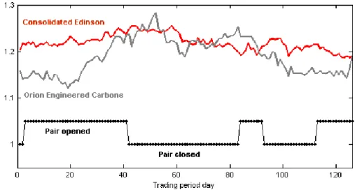
Figure 1: Normalized prices of Consolidated Edinson and Orion Engineered Carbons

This graph presents the evolution of Consolidated Edinson and Orion Engineered Carbons normalized prices, in the trading period from July to December 1963. The prices are normalized to one in the beginning of the formation period from July 1962 to June 1963. This pair is ranked in 12th_{, with a sum of squared deviations (SSD) of 0.1915.}

Figure 1 shows a real example of the trading period from July to December 1963, for the pair composed by Consolidated Edinson (ED) and Orion Engineered Carbons (OEC). The stocks move together showing their correlation, though they present small periods of divergence. The first positions are opened around day 2, by selling Consolidated Edinson, which has performed relatively better, and buying Orion Engineered Carbons, which has performed relatively worse. Around day 40, the prices cross and therefore we close the positions and realize a profit. The pair opens two more times, and in the second time, around day 85, opposite positions are executed, as this time Orion Engineered Carbons performs relatively better.

2.4. Performance

The gains and losses are computed by going one dollar long in the loser security and one dollar short in the winner security and thus each payoff is taken as an excess return. The excess return during the trading period is calculated based on the reinvested payoffs during this interval,

(11)

7 which is a conservative perspective for return calculation, as it assumes that the proceeds received during this interval are not earning any interest rate in the moments when the investor is waiting to open new positions. The daily excess returns are marked-to-market daily and then monthly compounded in order to obtain a series of monthly returns.

We evaluate the performance of pairs by computing two different excess return metrics: a. Return on Employed Capital (ROEC), that divides the payoffs by the number of pairs

that actually open during the trading period:

N ) r (r ROEC N 1 n long short



   (3)

where N represents the number of pairs in the portfolio and N the number of pairs that open during the trading period;

b. Return on Committed Capital (ROCC), that divides the payoffs by the total number of pairs in the portfolio. This metric provides a more conservative measure of excess return that takes into account the capital that investors have to commit to execute the pairs trading strategy, even if the positions do not open:

N ) r (r ROCC N 1 n long short



   (4)

In order to understand the risk exposure of the portfolios, we build two factor regressions. The first regression is used by Gatev et al (2006) and includes the Fama and French (2006) three factors, i.e. market, size and value, the Carhart (1997) momentum factor and the short-term reversal factor from Kenneth French website. This regression is represented by:

Rpt− Rft = αp+ β1(Rmt− Rft) + 𝛽2𝑆𝑀𝐵 + 𝛽3𝐻𝑀𝐿 + 𝛽3𝑀𝑂𝑀 + 𝛽4𝑅𝐸𝑉 + εpt (5) where Rpt denotes the portfolio monthly returns, Rft the risk-free rate (T-bill), Rmt the market factor, 𝑆𝑀𝐵 the small minus big (size) factor, 𝐻𝑀𝐿 the high minus low (value) factor, 𝑀𝑂𝑀 the momentum factor and 𝑅𝐸𝑉 the short-term reversal factor. As the pairs trading strategy is a

(12)

8 contrarian strategy, momentum and short-term reversal factors are key to its study. The former controls for the possibility that we are long on term winners and short on medium-term losers, and we expect a negative relation with the returns. The later controls for the possibility that we are long on short-term losers and short on short-term winners, and we expect a positive relation with the returns. The second regression is similar, but substitutes the short-term reversal factor by the Pastor and Stanbaugh (2003) liquidity factor represented by 𝐿𝐼𝑄:

Rpt− Rft = αp+ β1(Rmt− Rft) + 𝛽2𝑆𝑀𝐵 + 𝛽3𝐻𝑀𝐿 + 𝛽3𝑀𝑂𝑀 + 𝛽4𝐿𝐼𝑄 + εpt (6) This factor is relevant, as the returns of stocks sensitive to liquidity tend to be higher, as investors demand higher compensation for bearing liquidity risk (Pastor and Stanbaugh (2003)). Hence, we expect lower returns at times when aggregate liquidity is higher.

2.5. Decile formation

In order to evaluate the performance of different style investors, we form deciles in descending order, at the end of each formation period, based on:

a. Market capitalization, i.e. size;

b. Total compounded return during the formation period, i.e. momentum:

1 ) 1 ( R 1 1   



T_y t rt (7)

c. Formation period standard deviation, i.e. volatility.

2.6. Type of strategies

We execute three types of strategies:

a. Simple pairs trading (SPT) is the pure statistical arbitrage strategy;

b. Industry-restricted pairs trading (IRPT) is the strategy that only matches pairs within the same industry;

(13)

9 c. Size-restricted pairs trading (SRPT) is the strategy that only matches pairs within the

same size decile.

3. Results

3.1. Simple pairs trading

This section analyzes the simple pairs trading (SPT) strategy. From this section onwards, we consider the Top 5 and Top 20 portfolios as the pairs trading representatives, which are formed each 6 months with the 5 and 20 lowest pairs in SSD, respectively.

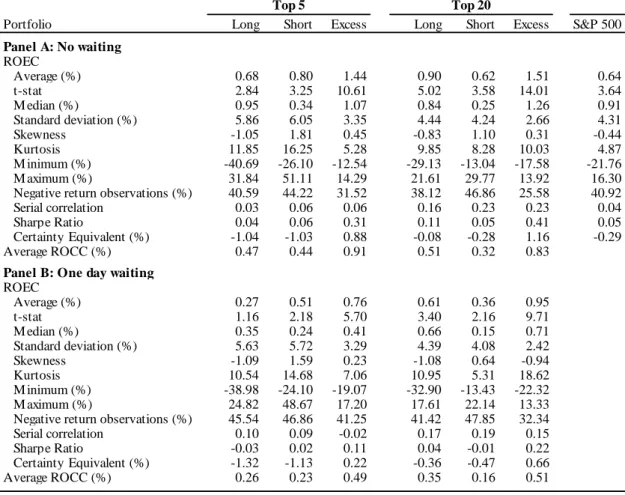
Table 1: Excess returns of the simple pairs trading strategy and S&P500

This table presents the monthly long positions, short positions and excess return descriptive statistics for different portfolios of pairs and the S&P500, between July 1963 and December 2013. We open positions in the pair when the two stocks diverge by more than 2 historical standard deviations and close the positions when they cross again. In Panel A, we execute the trades at the end of the day of divergence and/or convergence, i.e. no waiting rule, whereas in Panel B we postpone the trades by one day, i.e. one day waiting rule. The Top N portfolios include the N pairs matched by the least distance measure (SSD). ROEC stands for return on employed capital (scaled back by the number of pairs that opened) and ROCC for return on committed capital (scaled back by the total number of pairs that compose the portfolio). The Certain Equivalent is computed using the power utility function and a risk aversion coefficient of 5.

Portfolio Long Short Excess Long Short Excess S&P 500

Panel A: No waiting ROEC Average (%) 0.68 0.80 1.44 0.90 0.62 1.51 0.64 t-stat 2.84 3.25 10.61 5.02 3.58 14.01 3.64 M edian (%) 0.95 0.34 1.07 0.84 0.25 1.26 0.91 Standard deviation (%) 5.86 6.05 3.35 4.44 4.24 2.66 4.31 Skewness -1.05 1.81 0.45 -0.83 1.10 0.31 -0.44 Kurtosis 11.85 16.25 5.28 9.85 8.28 10.03 4.87 M inimum (%) -40.69 -26.10 -12.54 -29.13 -13.04 -17.58 -21.76 M aximum (%) 31.84 51.11 14.29 21.61 29.77 13.92 16.30

Negative return observations (%) 40.59 44.22 31.52 38.12 46.86 25.58 40.92

Serial correlation 0.03 0.06 0.06 0.16 0.23 0.23 0.04

Sharpe Ratio 0.04 0.06 0.31 0.11 0.05 0.41 0.05

Certainty Equivalent (%) -1.04 -1.03 0.88 -0.08 -0.28 1.16 -0.29

Average ROCC (%) 0.47 0.44 0.91 0.51 0.32 0.83

Panel B: One day waiting ROEC Average (%) 0.27 0.51 0.76 0.61 0.36 0.95 t-stat 1.16 2.18 5.70 3.40 2.16 9.71 M edian (%) 0.35 0.24 0.41 0.66 0.15 0.71 Standard deviation (%) 5.63 5.72 3.29 4.39 4.08 2.42 Skewness -1.09 1.59 0.23 -1.08 0.64 -0.94 Kurtosis 10.54 14.68 7.06 10.95 5.31 18.62 M inimum (%) -38.98 -24.10 -19.07 -32.90 -13.43 -22.32 M aximum (%) 24.82 48.67 17.20 17.61 22.14 13.33

Negative return observations (%) 45.54 46.86 41.25 41.42 47.85 32.34

Serial correlation 0.10 0.09 -0.02 0.17 0.19 0.15

Sharpe Ratio -0.03 0.02 0.11 0.04 -0.01 0.22

Certainty Equivalent (%) -1.32 -1.13 0.22 -0.36 -0.47 0.66

Average ROCC (%) 0.26 0.23 0.49 0.35 0.16 0.51

(14)

10 Table 1 presents the excess returns descriptive statistics of the SPT strategy. Between 1962 and 2013, the pairs trading strategy achieves higher reward and lower risk than the market. Both the Top 5 and Top 20 portfolios earn positive and significant excess returns, with outperforming average ROECs of respectively 1.44% and 1.51%, against a market average return of 0.64%. The same verifies for the more conservative measure ROCC of respectively 0.91% and 0.83%, and for Certainty Equivalents and Sharpe Ratios. It is evident that short positions have higher influence in the Top 5, whereas long positions have higher impact in the Top 20’s portfolio excess returns. The portfolios present a lower average standard deviation of respectively 3.35% and 2.66% against the market average of 4.31%.

The higher the number of pairs in a portfolio, the lower the standard deviation of returns and the higher the average excess returns, as we benefit from diversification. Though the skewness is lower in the Top 20 than in the Top 5 portfolio, the kurtosis is higher and there is a lower share of negative return observations (31.52% against 25.58%), meaning that we have a lower minimum but less chance that negative returns verify.

The same conclusions are taken when we postpone the trades by one day. Still, there is a drop in profitability, indicating that the bid-ask bounce influences the profits computed in Panel A. Even though the average ROCC is lower than the market average return, the SPT strategy beats in Sharpe Ratio and Certainty Equivalent, due to the lower standard deviation presented. It is noticeable that the SPT strategy was more profitable before 20021 and suffered a decline since then, presenting an average ROEC of 1.73%, between 1962 and 2002, against 1.44% in the Top 5 portfolio and 1.76% versus 1.51% in the Top 20 portfolio (no waiting rule). In the next subsections, we consider the one day waiting rule in order to analyze profitability conservatively.

1_{The results from 1962 to 2002 are not presented in the table due to lack of space, though we make them available}

(15)

11 Figure 2: Cumulative returns of Top 5, Top 20 and S&P500

Cumulative monthly returns, under the one day waiting rule, from July 1963 to December 2013 (ROEC in the case of the Top 5 and Top 20 portfolios).

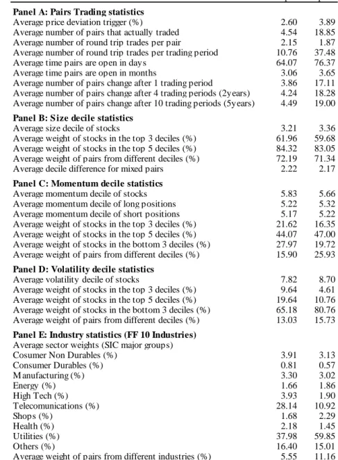
Figure 2 shows that, between 1963 and 2013, both the Top 5 and Top 20 portfolios have outperformed the S&P500 Composite Index. The performance of these portfolios was increasingly positive, not affected by crisis periods as the S&P500. In fact, during the market crash between 1972 and 1974, caused by the Oil and Bretton Woods’s crises, the Top 5 and Top 20 portfolios kept rising, whilst the S&P500 dropped. Likewise, during the 2007-2008 financial crisis, the SPT portfolios remained stable. The positive trend has slowed down in the last two decades for the Top 20 portfolio, whilst it turned slightly negative for the Top 5. Table 2 summarizes the trading statistics and portfolio composition of the SPT strategy between 1962 and 2013. As expected, the average price deviation trigger increases with the number of pairs in the portfolio, due to the lower closeness in the 5 to 20 top pairs, compared to the Top 5. On average, 4.54 pairs in the Top 5 portfolio and 18.85 pairs in the Top 20 portfolio end up opening positions during the trading period. These pairs tend to execute more than one roundtrip trade, showing an average of 2.15 and 1.87 roundtrips respectively, and to remain open 3.06 and 3.65 months on average, which is a positive signal for lower transaction costs than a common short-term strategy. The level of portfolio turnover is very high, with an

(16)

12 average of 3.86 pairs and 17.11 pairs substituted between trading periods, respectively. As predicted, the longer the period the higher the turnover, though the difference is small, with an average of 4.49 and 19 pairs substituted after 5 years.

Table 2: Portfolio and trading statistics of the simple pairs trading strategy

This table presents the portfolio composition and the trading statistics for different portfolios of pairs, between July 1963 and December 2013. The Top N portfolios include the N pairs matched by the least distance measure (SSD). Panel A presents the trading statistics, in which the average price deviation trigger is equal to 2 standard deviations of the historical difference between the stock prices of a given pair. The number of roundtrip trades equals the number of times the full trading strategy is executed (positions on the stocks of a pair opened and closed after a while). Panel B shows the portfolio composition by size (market capitalization) deciles. Panel C presents the portfolio composition by momentum deciles. Panel D describes the portfolio composition in volatility (formation period standard deviation) deciles. Finally, Panel E displays the industry composition of the portfolios.

Portfolio Top 5 Top 20

Panel A: Pairs Trading statistics

Average price deviation trigger (%) 2.60 3.89

Average number of pairs that actually traded 4.54 18.85

Average number of round trip trades per pair 2.15 1.87

Average number of round trip trades per trading period 10.76 37.48

Average time pairs are open in days 64.07 76.37

Average time pairs are open in months 3.06 3.65

Average number of pairs change after 1 trading period 3.86 17.11

Average number of pairs change after 4 trading periods (2years) 4.24 18.28

Average number of pairs change after 10 trading periods (5years) 4.49 19.00

Panel B: S ize decile statistics

Average size decile of stocks 3.21 3.36

Average weight of stocks in the top 3 deciles (%) 61.96 59.68

Average weight of pairs from different deciles (%) 72.19 71.34

Average decile difference for mixed pairs 2.22 2.17

Panel C: Momentum decile statistics

Average momentum decile of stocks 5.83 5.66

Average momentum decile of long positions 5.22 5.32

Average momentum decile of short positions 5.17 5.22

Average weight of stocks in the bottom 3 deciles (%) 27.97 19.72

Panel D: Volatility decile statistics

Average volatility decile of stocks 7.82 8.70

Average weight of stocks in the bottom 3 deciles (%) 65.18 80.76

Panel E: Industry statistics (FF 10 Industries) Average sector weights (SIC major groups)

Cosumer Non Durables (%) 3.91 3.13

Consumer Durables (%) 0.81 0.57 M anufacturing (%) 3.30 3.02 Energy (%) 1.66 1.86 High Tech (%) 3.93 1.90 Telecomunications (%) 28.14 10.92 Shops (%) 1.68 2.29 Health (%) 2.18 1.45 Utilities (%) 37.98 59.85 Others (%) 16.40 15.01

(17)

13 Panel B presents the size composition of the portfolios. The average size decile in the Top 5 and Top 20 portfolios is respectively 3.21 and 3.36, with 61.96% and 59.68% of the stocks in the top 3 size deciles and 84.32% and 83.05% in the top 5 size deciles, showing that the bulk of the portfolios is composed by big stocks. 72.19% and 71.34% of the Top 5 and Top 20 portfolios are mixed, with an average decile difference of 2.22 and 2.17 respectively. As big stocks on average present lower returns than small stocks (Barberis et al (2003), Banz (1981) and Fama and French (2012)), could the profits be higher if we match pairs of small stocks? Further, we study this possibility by performing the SPT strategy in each size decile.

Panel C shows the momentum decile composition of the portfolios. The average momentum decile of stocks is close to 6 in both the Top 5 and Top 20 portfolios. Contrary to expected, we reject the theory that reversal trading is in part responsible by the SPT strategy profitability. The long and short positions exhibit a close average momentum decile to the full sample and the average weight of pairs in different deciles is 15.90% and 25.93%, respectively.

Panel D summarizes the volatility composition of the portfolios. We find that most of the portfolio stocks have low-volatility. The average volatility decile in the Top 5 and the Top 20 portfolios is 7.82 and 8.70, with 65.17% and 80.76% of the stocks in the bottom 3 deciles, and only 7.82% and 8.70% in the top 3 deciles. This result is expected, since low-volatility stocks are more likely to be correlated to each other (Gatev et al (2006)).

Panel E shows the portfolio industry composition. In accordance to Gatev et al (2006), we find that most of the stocks are in the Utilities sector, with an average weight of 37.98% and 59.85% in the Top 5 and Top 20 portfolios. This was foreseeable, since the Utilities sector has low volatility due to the primary nature of its products. Telecommunications follows with much lower average weights of 28.14% and 10.92%, respectively. All the other sectors excluding Others present much lower average weights and have little relevance. In accordance to our

(18)

14 predictions, there is a low share of pairs composed by stocks in different industries (5.55% and 11.16% in the Top 5 and Top 20 portfolios).

Table 3 shows the risk exposure of the SPT portfolios, through the factor models. Looking at the R-squared’s, we find that none of the models explains the Top 5 and Top 20 portfolios’ profitability, meaning that the risk factors have little influence in the SPT strategy performance. Nonetheless, the model studied in Panel B has higher explanatory power.

Table 3: Risk exposure through factor Models of the simple pairs trading strategy

This table presents the Factor Model regressions of the monthly excess returns of the portfolios traded under the one day waiting rule, between July 1963 and December 2013. Panel A presents the regression coefficients for the model composed by the Fama-French market, size and value factors, Carhart momentum factor and the Kenneth French short-term reversal factor. Panel B presents the regression coefficients for the model, composed by the Fama-French market, size and value factors, Carhart momentum factor and the Pastor and Stambaugh liquidity factor. The strategy and market returns are net of the risk-free rate (T-bill returns). The t-statistic is presented between brackets, next to the correspondent coefficients. Portfolio Average ROEC (%) 0.76 (5.70) 0.95 (9.71) Panel A: Reversal Intercept (%) 0.36 (2.53) 0.54 (5.32) M arket -0.0081 (-0.24) 0.0024 (0.10) SM B -0.0309 (-0.68) 0.0721 (2.20) HM L 0.0137 (0.28) 0.0829 (2.31) M omentum -0.0227 (-0.68) -0.0733 (-3.07) Reversal 0.0242 (0.53) 0.0031 (0.09) (%) Panel B: Liquidity Intercept (%) 0.12 (0.76) 0.44 (3.85) M arket 0.0261 (0.78) 0.0154 (0.64) SM B -0.0201 (-0.45) 0.0758 (2.33) HM L 0.0221 (0.45) 0.0862 (2.41) M omentum -0.0181 (-0.57) -0.0701 (-3.04) Liquidity -0.0734 (-3.35) -0.0305 (-1.92) (%) 0.31 3.66 4.25 2.09 Top 5 Top 20 𝑅2 𝑅2 𝑅2

The risk-adjusted returns, i.e. intercepts, are significantly positive in Panel A, but in Panel B lose some of their significance, due to the substitution of the Reversal factor by the Liquidity factor. In the Top 5 portfolio, this is even sharper as the intercepts end up not significant. As expected, the market factor is insignificant in every portfolio and model, as the SPT strategy is market-neutral. The SMB and HML factors are insignificant in the Top 5 portfolio, and positive and significant (5% confidence level) in the Top 20 portfolio, meaning that both these factors are possible causes for the Top 20 portfolio’s slightly higher performance. The short-term reversal factor sign is in line with the expectations that some of the profits come from selling

(19)

15 short-term winners and buying short-term losers, though it is insignificant in both periods and portfolios. The Momentum factor sign is also consistent with the view that some of the profits come from selling medium-term winners and buying medium-term losers, though it is only significant in the Top 20 portfolio. This contributes to explain why the Top 20 portfolio outperform the Top 5 portfolio. Finally, the Liquidity factor coefficient is negative and significant in both periods and portfolios (1% and 10% confidence levels for Top 5 and Top 20, respectively), meaning that when aggregate liquidity is higher, the returns are lower as investors demand a lower liquidity premium.

3.2. Strategies comparison

In this subsection, we examine the two strategies that restrict each pair to the exact same characteristic: industry or size decile. Table 4 presents the results of the simple pairs trading (SPT), the industry-restricted pairs trading (IRPT) and the size-restricted pairs trading (SRPT) strategies.

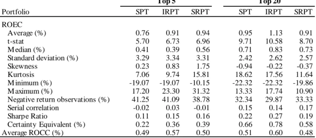
Table 4: Simple, industry restricted and size restricted pairs trading

This table presents the monthly excess returns descriptive statistics for different strategies, between July 1963 and December 2013. We open positions in the pair when the two stocks diverge by more than 2 historical standard deviations and close the positions when they cross again. Results correspond to the strategies executed under the one day waiting rule. The Top N portfolios include the N pairs matched by the least distance measure (SSD). ROEC stands for return on employed capital (scaled back by the number of pairs that opened) and ROCC for return on committed capital (scaled back by the total number of pairs). SPT stands for simple pairs trading, IRPT for industry-restricted pairs trading, that only matches pairs in the same industry, and SRPT for size-restricted pairs trading, that only matches pairs in the same size decile.

Portfolio SPT IRPT SRPT SPT IRPT SRPT

ROEC Average (%) 0.76 0.91 0.94 0.95 1.13 0.91 t-stat 5.70 6.73 6.96 9.71 10.58 8.70 M edian (%) 0.41 0.39 0.56 0.71 0.83 0.73 Standard deviation (%) 3.29 3.34 3.31 2.42 2.62 2.57 Skewness 0.23 0.83 1.75 -0.94 -0.22 -0.37 Kurtosis 7.06 9.74 15.81 18.62 17.56 11.64 M inimum (%) -19.07 -19.07 -10.15 -22.32 -22.32 -19.86 M aximum (%) 17.20 23.30 31.32 13.33 17.74 10.90

Serial correlation -0.02 0.03 -0.01 0.15 0.14 0.17

Sharpe Ratio 0.11 0.15 0.16 0.22 0.27 0.19

Certainty Equivalent (%) 0.22 0.36 0.39 0.66 0.78 0.58

Average ROCC (%) 0.49 0.57 0.50 0.51 0.60 0.48

(20)

16 The IRPT strategy outperforms the benchmark SPT strategy, in both portfolios. It presents higher average returns and higher standard deviations, though they only influence the positive side of the returns distribution. The maximums are higher, but the minimums are stable, which causes an increase in skewness and higher kurtosis in the Top 5 portfolio. The Sharpe Ratios and Certainty Equivalents are higher and there is a lower number of negative observations. When we execute this strategy, we take into account the fact that stocks in the same industry have permanent links and common factor exposures, and this may be the main cause for the IRPT higher performance.

We do not observe the same consistency for the SRPT strategy, which only outperforms the SPT strategy in the Top 5 portfolio under the one day waiting trading rule. When we consider the Top 5 and the Top 20 portfolios under the no waiting rule, this strategy presents lower average returns and higher standard deviations, with higher maximums and lower minimums, higher skewness, higher kurtosis and higher number of negative observations. 2 By restricting the pairs to the same size decile, we eliminate natural pairs with high interdependencies.

3.3. Pairs trading by industry

The SPT strategy matches stocks, which have moved closely in the formation period. Therefore, if stocks in different industries are highly correlated, there may be mixed-industry pairs in the SPT portfolios. Still, we find in the previous section that the share of pairs for which this mixed pairing happens is low. In order to understand if an industry-style investor can profit from this strategy, we individually execute the SPT strategy for the 10 Fama-French industries. The results are displayed in Table 5.

2_{Due to lack of space, we do not present the statistics for the no waiting rule, though we make them available in}

(21)

17 Table 5: Pairs trading by industry

This table presents the monthly long positions, short positions and excess returns descriptive statistics for all industries and each industry group, between July 1963 and December 2013. We open positions in the pair when the two stocks diverge by more than 2 historical standard deviations and close the positions when they cross again. Results correspond to the strategy executed under the one day waiting rule. The Top N portfolios include the N with the least distance measure (SSD). ROEC stands for return on employed capital (scaled back by the number of pairs that opened).

Portfolio Long Short Excess Long Short Excess

Panel A: All industries

Average ROEC (%) 0.27 0.51 0.76 0.61 0.36 0.95

t-stat 1.16 2.18 5.70 3.40 2.16 9.71

Sharpe Ratio -0.03 0.02 0.11 0.04 -0.01 0.22

Panel B: Consumer Non-Durables

Average ROEC (%) 1.22 -0.10 1.09 0.94 -0.13 0.79

t-stat 5.31 -0.49 5.21 4.45 -0.71 4.68

Sharpe Ratio 0.06 0.05 0.13 0.05 0.05 0.09

Panel C: Consumer Durables

Average ROEC (%) 0.78 0.29 1.06 0.74 0.17 0.82 t-stat 2.60 1.03 3.83 2.65 0.67 4.84 Sharpe Ratio 0.05 -0.02 0.09 0.05 -0.04 0.10 Panel D: Manufacturing Average ROEC (%) 0.59 0.12 0.68 0.69 -0.07 0.58 t-stat 2.46 0.47 3.44 3.01 -0.31 4.43 Sharpe Ratio 0.03 -0.05 0.05 0.05 -0.09 0.05 Panel E: Energy Average ROEC (%) 0.96 -0.50 0.45 0.77 -0.40 0.39 t-stat 3.10 -1.80 2.10 2.73 -1.54 2.60 Sharpe Ratio 0.07 -0.13 0.01 0.05 -0.13 -0.01

Panel F: High Tech

Average ROEC (%) 0.35 -0.24 0.06 0.68 0.02 0.60 t-stat 1.04 -0.84 0.22 2.20 0.09 3.10 Sharpe Ratio -0.01 -0.09 -0.05 0.04 -0.06 0.04 Panel G: Telecomunications Average ROEC (%) 0.64 -0.07 0.57 0.76 0.05 0.81 t-stat 2.52 -0.30 3.25 3.12 0.26 4.23 Sharpe Ratio 0.04 -0.08 0.04 0.06 -0.07 0.08 Panel H: S hops Average ROEC (%) 1.02 0.13 1.12 0.82 0.06 0.82 t-stat 3.90 0.55 4.84 3.52 0.25 4.97 Sharpe Ratio 0.09 -0.05 0.12 0.07 -0.07 0.10 Panel I: Health Average ROEC (%) 0.91 -0.54 0.37 0.94 -0.30 0.63 t-stat 3.87 -2.44 1.86 4.14 -1.43 3.66 Sharpe Ratio 0.09 -0.18 -0.01 0.09 -0.14 0.05 Panel J: Utilities Average ROEC (%) 0.58 0.28 0.84 0.66 0.38 1.01 t-stat 3.30 1.57 5.84 3.77 2.36 9.48 Sharpe Ratio 0.04 -0.03 0.12 0.06 -0.01 0.23 Panel K: Others Average ROEC (%) 0.60 0.08 0.61 0.84 0.04 0.86 t-stat 2.35 0.30 3.42 3.73 0.18 6.80 Sharpe Ratio 0.03 -0.05 0.04 0.08 -0.08 0.14 Top 5 Top 20

The Utilities industry group is the only one that presents higher average excess returns than the full sample of industries, in both portfolios. Both the Top 5 and Top 20 portfolios yield significant 0.84% and 1.01% average ROECs, and 0.12 and 0.23 Sharpe ratios. This result is

(22)

18 in line with Gatev et al (2006) that presents the Utilities sector as the most profitable between 1962 and 2002. In the Top 5 portfolio, the Consumer Non-Durables, Consumer Durables and Shops present higher average ROEC than the full sample and the Utilities sector it-self, with respectively 1.09%, 1.06% and 1.12% average ROECs. Nonetheless, the Sharpe Ratios are similar and the Utilities Top 20 portfolio is the only to outperform the full sample Top 20 portfolio. Energy, High Tech and Health present the lowest results of the Top 5 portfolio, whereas Energy, High Tech and Manufacturing have the lowest results of the Top 20. These sectors are highly affected by their short positions, which present negative average ROECs. All the industries show positive and significant excess returns, meaning that an industry style investor is able to profit from the SPT strategy, no matter his industry preferences.

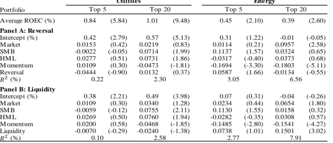
Table 6 analyzes the risk exposure of the Utilities sector, against the Energy sector. We take these two sectors, due to their distinct volatility levels, i.e. Utilities is a low volatility sector whereas Energy is high, as well as their different levels of profitability in the previous analysis. Table 6: Risk exposure through factor models for the Utilities and Energy sectors

This table presents the Factor Model regressions for the monthly excess returns of the Utilities and Energy portfolios, traded under the one

day waiting rule, between July 1963 and December 2013. Panel A presents the regression coefficients for the model composed by the

Fama-French market, size and value factors, Carhart momentum factor and the Kenneth Fama-French short-term reversal factor. Panel B presents the regression coefficients for the model, composed by the Fama-French market, size and value factors, Carhart momentum factor and the Pastor and Stambaugh liquidity factor. The strategy and market returns are net of the risk-free rate (T-bill returns). The t-statistic is presented between brackets, next to the correspondent coefficients.

Portfolio Average ROEC (%) 0.84 (5.84) 1.01 (9.48) 0.45 (2.10) 0.39 (2.60) Panel A: Reversal Intercept (%) 0.42 (2.79) 0.57 (5.13) 0.31 (1.22) -0.01 (-0.05) M arket 0.0153 (0.42) 0.0219 (0.83) 0.0114 (0.21) 0.0957 (2.58) SM B -0.0022 (-0.05) 0.0714 (1.99) 0.1137 (1.57) 0.0324 (0.65) HM L 0.0277 (0.51) 0.0731 (1.86) -0.0317 (-0.40) 0.0373 (0.68) M omentum 0.0109 (0.30) -0.0473 (-1.81) -0.1694 (-3.30) -0.1803 (-5.11) Reversal -0.0444 (-0.90) 0.0132 (0.37) 0.0587 (1.66) -0.0134 (-0.55) (%) Panel B: Liquidity Intercept (%) 0.38 (2.21) 0.49 (3.98) 0.07 (0.31) -0.04 (-0.26) M arket 0.0109 (0.30) 0.0340 (1.28) 0.0234 (0.44) 0.0654 (1.80) SM B -0.0059 (-0.12) 0.0755 (2.11) 0.1130 (1.55) 0.0158 (0.32) HM L 0.0269 (0.50) 0.0760 (1.94) -0.0282 (-0.35) 0.0308 (0.57) M omentum 0.0200 (0.58) -0.0468 (-1.85) -0.1485 (-2.80) -0.1541 (-4.27) Liquidity -0.0070 (-0.29) -0.0240 (-1.38) 0.0738 (1.01) 0.1501 (3.02) (%) Utilities Energy 0.10 2.58 2.77 7.91

Top 5 Top 20 Top 5 Top 20

0.22 2.30 3.05 6.56

𝑅2

(23)

19 Once again, we find that none of the models explains in detail the Top 5 and Top 20 portfolios profitability for neither the Utilities nor the Energy sector, and therefore these risk factors have little influence in the SPT strategy performance. Nonetheless, Panel B’s model have higher explanatory power in the Top 20, whereas Panel A’s fits better the Top 5.

In accordance to the full sample factor analysis, the risk-adjusted returns in the Utilities sector are significantly positive in Panel A, whereof lose some of their significance in Panel B. As predicted, the alphas are lower in the Energy than in the Utilities sectors, and the Energy sector is not significant in both Panel A and B (10% confidence level). The market factor is insignificant in every portfolio and sector, due to the strategy’s market-neutrality. For the Utilities portfolios, we find that the size and value factors are insignificant in the Top 5, but positive and significant in the Top 20 (5% confidence level for the size factor and 10% for the value factor). The short-term reversal factor is insignificant in the Utilities Top 5 and Top 20 and in the Energy Top 20, but positive and significant (10% significance level) in the Energy Top 5. The momentum factor is negative and significant in the Top 20 Utilities (10% confidence level) and Top 5 and Top 20 Energy portfolios (1% confidence level), in line with our beliefs. Finally, the Liquidity coefficient is positive and significant in the Energy Top 20 portfolio (1% confidence level), but insignificant in the remaining portfolios.

Overall, the Utilities sector has lower R-squared’s than the Energy sector, meaning that it is explained by the models at a lower degree. The fact that it is less impacted by the risk factors may be what causes its higher profitability.

3.4. Pairs trading in the S&P500 Composite Index

In order to understand whether the SPT strategy is profitable for investors that prefer blue chip/big stocks, we analyze the results of the SPT strategy restricted to the members of the S&P500 Composite Index. Table 7 shows the results.

(24)

20 Table 7: Simple pairs trading strategy restricted of the S&P500 stocks

This table presents the monthly excess return descriptive statistics of the SPT strategy restricted to the S&P500 members, under the one day

waiting and no waiting rules, between July 1963 and December 2013. We open positions in the pair when the two stocks diverge by more

than 2 historical standard deviations and close the positions when they cross again. The Top N portfolios include the N pairs matched by the least distance measure (SSD). ROEC stands for return on employed capital (scaled back by the number of pairs that opened) and ROCC for return on committed capital (scaled back by the total number of pairs that compose the portfolio). The Certain Equivalent is computed using the power utility function and a risk aversion coefficient of 5.

Portfolio Top 5 Top 20 Top 5 Top 20 S&P 500

ROEC Average (%) 0.96 1.11 0.68 0.81 0.64 t-stat 5.90 9.76 4.33 7.68 3.64 M edian (%) 0.57 0.90 0.44 0.69 0.91 Standard deviation (%) 4.00 2.81 3.87 2.58 4.31 Skewness -0.07 0.44 -1.13 -0.02 -0.44 Kurtosis 12.78 9.32 18.82 9.38 4.87 M inimum (%) -31.39 -16.91 -36.86 -17.39 -21.76 M aximum (%) 20.32 15.46 16.67 15.35 16.30

Negative return observations (%) 41.25 34.32 43.56 37.62 40.92

Serial correlation 0.11 0.18 0.14 0.16 0.04

Sharpe Ratio 0.14 0.25 0.07 0.15 0.05

Certainty Equivalent (%) 0.16 0.72 -0.07 0.47 -0.29

Average ROCC (%) 0.46 0.55 0.29 0.39

No waiting One day waiting

The SPT strategy makes sense to investors that restrict their portfolios to big and reputed stocks. Under the no waiting rule, we get positive and significant average ROECs of 0.96% in the Top 5 portfolio and 1.11% in the Top 20 portfolio against 0.64% in the S&P500 Composite Index, and outperforming Sharpe Ratios and Certainty Equivalents. The same conclusions verify under the one day waiting trading rule.

Nevertheless, the performance decreases when compared with non-restricted SPT strategy, as the investors lose proceeds from high interdependencies of smaller-sized stocks. The inferences are similar when we consider the conservative ROCC metric.

3.5. Pairs trading by size

Many investors consider size when composing their portfolios. Small stocks are expected to have higher returns (Banz (1981) and Fama and French (2012)), whereas big stocks have stronger reputation and are liquid (Del Guercio (1996) and Falkenstein (1996)). In this subsection, we analyze this risk-return tradeoff that investors face during the portfolio

(25)

21 formation, by examining the SPT strategy in each size decile. In table 8, we present a breakdown of the pairs trading by relevant size deciles.

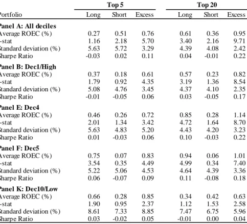
Table 8: Pairs trading by size

This table presents the monthly long positions, short positions and excess returns descriptive statistics of the SPT strategy (All deciles) and of the relevant size deciles (High, Dec4, Dec5 and Low deciles), between July 1963 and December 2013. Results correspond to the strategy executed under the one day waiting rule. The decile portfolios are presented in descending order: decile 1 (High) is composed by the biggest stocks, whereas decile 10 (Low) by the smallest. We open positions in the pair when the two stocks diverge by more than 2 historical standard deviations and close the positions when they cross again. The Top N portfolios include the N pairs matched by the least distance measure (SSD). ROEC stands for return on employed capital (scaled back by the number of pairs that opened) and ROCC for return on committed capital (scaled back by the total number of pairs that compose the portfolio).

Portfolio Long Short Excess Long Short Excess

Panel A: All deciles

Average ROEC (%) 0.27 0.51 0.76 0.61 0.36 0.95 t-stat 1.16 2.18 5.70 3.40 2.16 9.71 Standard deviation (%) 5.63 5.72 3.29 4.39 4.08 2.42 Sharpe Ratio -0.03 0.02 0.11 0.04 -0.01 0.22 Panel B: Dec1/High Average ROEC (%) 0.37 0.18 0.61 0.57 0.23 0.82 t-stat 1.79 0.92 4.35 3.19 1.36 8.54 Standard deviation (%) 5.08 4.76 3.45 4.37 4.10 2.35 Sharpe Ratio -0.01 -0.05 0.06 0.03 -0.05 0.17 Panel E: Dec4 Average ROEC (%) 0.46 0.26 0.72 0.85 0.28 1.14 t-stat 2.01 1.34 3.42 4.72 1.64 8.70 Standard deviation (%) 5.63 4.83 5.20 4.43 4.20 3.23 Sharpe Ratio 0.01 -0.03 0.06 0.10 -0.03 0.22 Panel F: Dec5 Average ROEC (%) 0.75 0.07 0.83 0.94 0.06 1.01 t-stat 3.54 0.35 4.49 4.99 0.34 7.40 Standard deviation (%) 5.22 5.06 4.53 4.64 4.39 3.36 Sharpe Ratio 0.06 -0.07 0.09 0.11 -0.08 0.18 Panel K: Dec10/Low Average ROEC (%) 0.66 0.28 0.85 0.34 0.42 0.63 t-stat 1.90 0.95 2.37 1.12 1.53 2.58 Standard deviation (%) 8.61 7.33 8.85 7.47 6.75 5.96 Sharpe Ratio 0.03 -0.02 0.05 -0.01 0.00 0.04 Top 5 Top 20

Dec5 is the only that presents higher average excess returns in both the Top 5 and Top 20 than the full sample, with significant average ROECs of 0.83% and 1.01%, respectively. In the Top 5 portfolio, Dec6, Dec9 and Dec10 all present higher average ROEC than the full sample, with respectively 0.93%, 1.05% and 0.85% average ROECs. In the Top 20, besides Dec5, also Dec4 beats the full sample. Dec8 is the worst performing decile, followed by Dec2. 3 When we consider the Sharpe Ratios, we find that no size decile outperforms the full sample, which

3_{Due to lack of space, we do not present the statistics for all the deciles, though we make them available in an}

(26)

22 indicates that trading pairs in the same size decile is not be the best option, since we eliminate pairs with high interdependencies from the investment set.

We conclude that if we were to invest in one size decile it would be Decile 5 (one of the middle deciles). The fact that the excess returns are positive and significant is predominant across the whole series of deciles, attesting once again the robustness of this strategy and the ability of size style investors to profit from the SPT strategy.

3.6. Momentum pairs trading

Some investors prefer to invest in momentum stocks, which have shown recent positive performance (Falkenstein (1996)). In this subsection, we restrict the SPT strategy to the top 3 momentum deciles (MT3), and compare it to the bottom 3 momentum deciles (MB3). The descriptive statistics are presented in Table 9.

Table 9: Momentum pairs trading

This table presents the monthly excess returns descriptive statistics of different momentum strategies, under the one day waiting rule, between July 1963 and December 2013. We open positions in the pair when the two stocks diverge by more than 2 historical standard deviations and close the positions when they cross again. The Top N portfolios include the N pairs matched by the least distance measure (SSD). ROEC stands for return on employed capital (scaled back by the number of pairs that opened) and ROCC for return on committed capital (scaled back by the total number of pairs). MT3 and MB3 stand for pairs trading restricted to the top 3 and bottom 3 momentum deciles, respectively.

Portfolio M T3 M B3 M T3 M B3 ROEC Average (%) 0.67 0.35 0.78 0.86 t-stat 4.10 1.62 6.84 4.84 M edian (%) 0.32 0.49 0.75 0.76 Standard deviation (%) 4.04 5.28 2.81 4.38 Skewness 0.37 -0.36 0.06 0.52 Kurtosis 5.60 6.98 4.20 9.71 M inimum (%) -20.11 -28.87 -9.84 -21.55 M aximum (%) 17.54 23.63 12.79 28.82

Negative return observations (%) 43.73 44.39 38.12 40.76

Serial correlation 0.07 -0.01 0.04 0.04

Sharpe Ratio 0.06 -0.01 0.13 0.10

Certainty Equivalent (%) -0.14 -1.05 0.39 -0.10

Average ROCC (%) 0.40 0.17 0.50 0.17

Top 5 Top 20

We find that momentum style investors earn significantly positive returns with the SPT strategy. Investors that prefer winner stocks present superior performance than investors persuaded for loser stocks, and can profit with the Top 20 portfolio. Nonetheless, both the

(27)

23 styles of investing underperform the SPT benchmark, meaning that investors are worse off by restricting the sample of stocks to past one-year winners or past one-year losers.

3.7. Volatility pairs trading

In this subsection, we restrict the SPT strategy to the top 3 (VT3), top 5 (VT5), bottom 5 (VB5) and bottom 3 (VB3) volatility deciles, in order to study the risk-return trade-off. The results are summarized in Table 10.

Table 10: Volatility pairs trading

This table presents the monthly excess returns descriptive statistics of different volatility strategies, under the one day waiting rule, between July 1963 and December 2013. We open positions in the pair when the two stocks diverge by more than 2 historical standard deviations and close the positions when they cross again. The Top N portfolios include the N pairs matched by the least distance measure (SSD). ROEC stands for return on employed capital (scaled back by the number of pairs that opened) and ROCC for return on committed capital (scaled back by the total number of pairs). VT3 and VT5 stand for pairs trading restricted to the top 3 and top 5 volatility deciles, respectively, whereas VB3 and VB5 stand for pairs trading restricted to the bottom 3 and bottom 5 volatility deciles.

Portfolio VT3 VT5 VB5 VB3 VT3 VT5 VB5 VB3 ROEC Average (%) 1.23 0.23 0.74 0.76 0.88 0.83 0.94 0.93 t-stat 3.83 1.01 5.63 5.51 3.63 5.43 9.53 9.34 M edian (%) 0.60 0.00 0.40 0.36 0.48 0.70 0.71 0.70 Standard deviation (%) 7.93 5.72 3.22 3.39 5.98 3.76 2.42 2.45 Skewness 0.58 0.05 -0.02 0.72 -0.03 -0.01 -0.98 -0.68 Kurtosis 9.40 7.41 6.64 10.93 8.71 5.60 17.77 18.53 M inimum (%) -36.72 -29.29 -19.07 -19.07 -31.70 -20.18 -22.32 -22.32 M aximum (%) 50.56 30.97 13.23 26.92 29.62 14.93 11.67 16.17

Negative return observations (%) 43.56 49.01 40.92 41.91 43.40 40.76 32.84 34.16

Serial correlation -0.01 -0.03 -0.02 0.00 0.00 -0.03 0.16 0.13

Sharpe Ratio 0.10 -0.03 0.10 0.10 0.08 0.11 0.22 0.21

Certainty Equivalent (%) -1.91 -1.40 0.22 0.18 -0.91 0.12 0.64 0.63

Average ROCC (%) 0.65 0.24 0.50 0.45 0.39 0.41 0.50 0.50

Top 5 Top 20

We find that no strategy outperforms the SPT strategy. In fact, when we consolidate all the statistics and analyze the Certainty Equivalent, we find that bottom volatility restricted strategies outperform top volatility restricted strategies, which contests the risk-return tradeoff theory.

Nevertheless, there is consistency for positive and significant excess returns across all volatility deciles, meaning that volatility style investors are able to ear positive returns from the SPT strategy. However, if we consider Sharpe Ratios and Certainty Equivalents, investors can only achieve this profitability if they take the Top 20 portfolio.

(28)

24

4. Robustness

4.1. Period Analysis

This subsection examines the robustness of the SPT strategy to different periods. Table 11 shows the results.

Table 11: Simple pairs trading by periods

This table presents the monthly excess returns descriptive statistics in five different periods: Jul 1963 – Dec 1973 (Panel A), Jan 1974 – Dec 1983 (Panel B), Jan 1984 – Dec 1993 (Panel C), Jan 1994 – Dec 2003 (Panel D) and Jan 2004 – Dec 2013 (Panel E). Results are presented under the no waiting and the one day waiting rules. We open positions in the pair when the two stocks diverge by more than 2 historical standard deviations and close the positions when they cross again. The Top N portfolios include the N pairs matched by the least distance measure (SSD). ROEC stands for return on employed capital (scaled back by the number of pairs that opened) and ROCC for return on committed capital (scaled back by the total number of pairs that compose the portfolio).

Portfolio Top 5 Top 20 Top 5 Top 20

Panel A: Jul 1963 - Dec 1973

Average ROEC (%) 1.59 2.07 1.17 1.40

t-stat 5.01 9.39 3.77 7.14

Sharpe Ratio 0.33 0.68 0.22 0.45

Panel B: Jan 1974 - Dec 1983

Average ROEC (%) 2.14 2.57 1.63 1.82

t-stat 6.01 7.81 4.73 5.68

Sharpe Ratio 0.37 0.52 0.25 0.32

Panel C: Jan 1984 - Dec 1993

Average ROEC (%) 1.71 1.67 0.86 1.03

t-stat 5.26 8.63 2.75 6.02

Sharpe Ratio 0.34 0.54 0.10 0.28

Panel D: Jan 1994 - Dec 2003

Average ROEC (%) 1.37 0.67 0.27 0.15

t-stat 4.71 3.12 0.87 0.82

Sharpe Ratio 0.32 0.14 -0.02 -0.09

Panel E: Jan 2004 - Dec 2013

Average ROEC (%) 0.40 0.57 -0.15 0.35

t-stat 2.22 3.32 -1.03 2.33

Sharpe Ratio 0.14 0.24 -0.18 0.14

No waiting One day waiting

We find a significant decrease in performance in the last two decades, especially in the period from Jan 2004 to Dec 2013. Under the no waiting trading rule, the SPT strategy yields positive and significant excess returns and positive Sharpe Ratios, in all the portfolios and periods. Under the one day waiting trading rule however, in the last two decades, the Top 5 portfolio’s average ROECs are insignificant and the Sharpe Ratios are negative. The Top 20’s average ROECs are positive but insignificant in the period between Jan 1994 and Dec 2003.

We conclude that in general the Top 20 portfolio is robust to different periods, whereas the Top 5 portfolio is not.

(29)

25

4.2. Expansion and recession periods

In this subsection, we analyze the robustness of the SPT strategy to expansion and recession periods between July 1963 and December 2013, categorized by the National Bureau of Economic Research for the US economy.

Table 12: Simple pairs trading during expansion and recession periods

This table presents the monthly excess returns descriptive statistics during expansion and recession periods, characterized by the National Bureau of Economic Research for the US economy, between July 1963 and December 2013. Results correspond to the strategy executed under the one day waiting rule. We open positions in the pair when the two stocks diverge by more than 2 historical standard deviations and close the positions when they cross again. The Top N portfolios include the N pairs matched by the least distance measure (SSD). ROEC stands for return on employed capital (scaled back by the number of pairs that opened) and ROCC for return on committed capital (scaled back by the total number of pairs that compose the portfolio).

ROEC Average (%) 0.60 0.83 1.66 1.65 t-stat 4.43 9.07 3.84 4.19 M edian (%) 0.36 0.60 0.92 1.80 Standard deviation (%) 3.10 2.08 4.10 3.75 Skewness 0.06 0.39 0.38 -2.51 Kurtosis 8.12 5.54 3.85 20.75 M inimum (%) -19.07 -9.17 -10.91 -22.32 M aximum (%) 17.20 10.09 13.23 13.33

Serial correlation -0.07 0.12 0.02 0.13

Sharpe Ratio 0.07 0.21 0.27 0.30

Certainty Equivalent (%) 0.12 0.61 0.82 0.95

Average ROCC (%) 0.40 0.44 1.02 0.89

Expansions Recessions

Table 12 presents the average descriptive statistics in both expansion and recession periods. The SPT excess returns are significantly positive both in expansion and recession periods, though significantly higher in recessions. As expected, the standard deviation is also higher, but the average returns’ scale is bigger, which is reflected in the higher Sharpe Ratios. In the Top 5 portfolio the skewness is higher in recession periods, whereas in the Top 20 is lower. There is a lower percentage of negative return observations in both portfolios in recession than in expansion periods, which is the main causer for the higher performance of recessions.

4.3. Transaction costs

In this subsection, we examine the robustness of the SPT strategy to transaction costs. As the SPT strategy is dynamic, it is crucial to understand if the trading costs have influence on its

(30)

26 profits. Therefore, we deduct a transaction fee each time positions are opened or closed. We consider two different fees: 0.1% and 1%. The descriptive statistics are showed in Table 13. Table 13: Simple pairs trading with transaction costs

This table presents the monthly excess return descriptive statistics of the SPT strategy with transaction costs, under the no waiting rule, between July 1963 and December 2013. We open positions in the pair when the two stocks diverge by more than 2 historical standard deviations and close the positions when they cross again. The Top N portfolios include the N pairs matched by the least distance measure (SSD). ROEC stands for return on employed capital (scaled back by the number of pairs that opened) and ROCC for return on committed capital (scaled back by the total number of pairs that compose the portfolio). The Certain Equivalent is computed using the power utility function and a risk aversion coefficient of 5. We consider two different transactions fees: 0.1% and 1%.

ROEC Average (%) 1.32 1.41 0.17 0.45 t-stat 9.81 13.15 1.37 4.39 M edian (%) 0.95 1.13 0.00 0.28 Standard deviation (%) 3.30 2.64 3.08 2.52 Skewness 0.44 0.29 0.24 -0.01 Kurtosis 5.37 10.17 5.60 10.27 M inimum (%) -12.54 -17.68 -12.54 -18.58 M aximum (%) 14.23 13.53 13.72 12.11

Serial correlation 0.05 0.22 -0.04 0.10

Sharpe Ratio 0.27 0.38 -0.08 0.01

Certainty Equivalent (%) 0.77 1.06 -0.30 0.13

Average ROCC (%) 0.83 0.83 0.13 0.15

TC=0.1% TC=1%

The SPT Top 5 and Top 20 portfolios remain profitable when we consider a 0.1% transaction fee, with positive and significant average ROECs and positive Sharpe Ratios and Certainty Equivalents. However, when we consider a 1% transaction fee, the Top 5 portfolio ROEC loses significance and the Sharpe Ratio and the Certainty Equivalent are negative, whereas the Top 20 remains profitable but at a much lower degree.

We conclude that SPT strategy is profitable and outperforms the benchmark index for investors that face low transaction costs, usually institutional and investment banks, whereas we do not confirm this performance for individual investors that face higher transaction costs.

4.4. Trigger analysis

This subsection analyzes the robustness of the SPT strategy to different triggers. We open positions when the two stocks diverge by more than 1, 2 and 3 (Trig1, Trig 2 and Trig3) historical standard deviations.

(31)

27 Table 14: Simple pairs trading under different trigger rules

This table presents the monthly excess returns descriptive statistics of the SPT strategy executed under different trigger rules for the opening of positions, between July 1963 and December 2013. Results are presented under the no waiting rule. The Top N portfolios include the N pairs matched by the least distance measure (SSD). We open positions in the pair when the two stocks diverge by more than 1 (Trig1), 2 (Trig2) and 3 (Trig3) historical standard deviations and close the positions when they cross again. ROEC stands for return on employed capital (scaled back by the number of pairs that opened) and ROCC for return on committed capital (scaled back by the total number of pairs that compose the portfolio).

Trig1 Trig2 Trig3 Trig1 Trig2 Trig3

ROEC Average (%) 1.00 0.76 0.69 1.07 0.95 0.90 t-stat 8.63 5.70 5.09 13.06 9.71 7.70 M edian (%) 0.63 0.41 0.20 0.94 0.71 0.76 Standard deviation (%) 2.84 3.29 3.35 2.02 2.42 2.88 Skewness 0.62 0.23 0.29 0.56 -0.94 -1.12 Kurtosis 6.95 7.06 7.01 10.86 18.62 14.91 M inimum (%) -11.50 -19.07 -16.05 -11.94 -22.32 -25.45 M aximum (%) 16.74 17.20 18.93 14.02 13.33 11.01

Serial correlation 0.00 -0.02 -0.05 0.26 0.15 0.11

Sharpe Ratio 0.20 0.11 0.08 0.33 0.22 0.17

Certainty Equivalent (%) 0.59 0.22 0.13 0.87 0.66 0.49

Average ROCC (%) 0.80 0.49 0.33 0.82 0.51 0.31

Top 5 Top 20

Table 14 shows that the lower the trigger, the higher the average ROEC and ROCC and the lower the standard deviation in both portfolios, which generates higher Sharpe Ratios. The Certainty Equivalent metric is also consistent with this view. In fact, also the skewness is progressively higher, meaning that the pairs trading investor gets higher exposition to the positive than to the negative side, and the number of negative return observations drops (except when we consider the difference between Trigger 1 and Trigger 2 in the Top 5 portfolio). As expected, the higher the trigger lower the number of pairs that actually open and the shorter the period that the pairs remain open. 4_{For Trigger 1, the average number of pairs that actually} traded is 4.98 in the Top 5 and 19.89 in the Top 20 portfolios, and they are on average open 4.50 and 4.82 months, respectively. For Trigger 3, the average number of pairs that traded is 3.52 in the Top 5 and 16.04 in the Top 20 portfolios, and they are on average open 2.03 and 2.60 months, respectively.

4_{Due to lack of space, we do not present the trading statistics for different triggers, though we make them available}

(32)

28 The results show that this strategy is robust to any of the three triggers implemented, as the average ROEC and ROCC are positive and significant in both portfolios. We significantly increase the SPT strategy performance when we select the one standard deviation trigger.

5. Conclusions

In accordance to Gatev et al (2006) and Do and Faff (2010), we find that the pairs trading strategy registered a positive trend in profits between 1962 and 2013, which has been slowing down in the last two decades. We observe that this strategy presents a particular aptitude to capture superior returns in periods of crisis. However, not all the investors are able to benefit from these profits. Investors that execute trades in large scale, such as institutional and investment banks, trade at low transaction costs and benefit from the pairs trading strategy, whilst individual investors may not profit due to high transaction fees.

We find that style investing is profitable for any size, industry, momentum or volatility preferences. Yet, Utilities investors are the only to outperform the statistical arbitrage benchmark, meaning that the other investors achieve superior performance if they do not restrict the matching opportunities.

Foremost, we find that the initial stock matches improve when we execute a strategy that only matches same-industry stocks, which outperforms the general pairs trading strategy. Stocks in the same industry are more likely to keep moving together than stocks from different industries. While mixed-industry pairs present higher correlation in certain periods, sometimes this correlation is temporary, contrasting with same-industry pairs that are likely to keep their correlation.

(33)

29

References

Banz, R.W., 1981. The relationship between return and market value of common stocks. Journal of Financial Economics 9, 3–18.

Barberis, N., Schleifer, A., 2003. Style investing. Journal of Financial Economics 68, 161-199.

Carhart, M.M., 1997. On persistence in mutual fund performance. Journal of Finance 52, 57–82.

Cavaglia, S., Brightman, C., Aked, M., 2000. The increasing importance of industry factors. Financial Analysts Journal 56, 41-54.

Chan, L. K. C.,Lakonishok, J., Swaminathan, B., 2007. Industry classifications and return comovement. Financial Analysts Journal 63, 56-70.

Choi, N., Sias, R. W., 2009. Institutional industry herding. Journal of Financial Economics 94, 469-491.

Do, B., Faff, R., 2010. Does simple pairs trading still work? Financial Analysts Journal 66, 83-95.

De Bondt, W.F.M., Thaler, R.H., 1985. Does the stock market overreact? Journal of Finance 40, 793–805.

Del Guercio, D., 1996. The distorting effect of prudent-man laws on institutional equity investments. Journal of Financial Economics 40, 31-62.

Falkenstein, E., 1996. Preferences for stock characteristics as revealed by mutual fund portfolio holdings. Journal of Finance 51, 111-135.

Fama, E.F., French, K.R., 1996. Multifactor explanations of asset pricing anomalies. Journal of Finance 51, 55– 84.

Fama, E.F., French, K.R., 2012. Size, value, and momentum in international stock returns. Journal of Financial Economics 105, 457-472.

Gatev, E., Goetzmann, W.N. and Rouwenhorst, K.G., 2006. Pairs trading: Performance of a relative-value arbitrage rule. The Review of Financial Studies 19, 797-827.

Jegadeesh, N., Titman, S., 1993. Returns to buying winners and selling losers: Implications for stock market efﬁciency. Journal of Finance 48, 65–91.

Lundblad, C., 2007. The risk return tradeoff in the long run: 1836–2003. Journal of Financial Economics 85, 123-150.

Moskowitz, T., Grinblatt, M., 1999. Do industries explain momentum? Journal of Finance 54, 1249–1290.

Pastor, L., Stambaugh, R.F., 2003. Liquidity risk and expected stock returns. Journal of Political Economy 111, 642–685.