Stefano Beretta
1;2stefano.beretta@disco.unimib.it (+39)02 6448 7832
Mauro Castelli
3mcastelli@novaims.unl.pt (+351)213 828 610
Ivo Gonçalves
3;4igoncalves@novaims.unl.pt (+351)213 828 206
Ivan Kel
2ivan.kel@itb.cnr.it (+39)02 2642 2606
Valentina Giansanti
2valentina.giansanti@itb.cnr.it (+39)02 2642 2606
Ivan Merelli
2;⋆ ivan.merelli@itb.cnr.it (+39)02 2642 2606
Addresses:
1 Dipartimento di Informatica Sistemistica e Comunicazione, Universit a degli
Studi di Milano-Bicocca, Viale Sarca 336, 20126 Milan, Italy.
2 Istituto di Tecnologie Biomediche, Consiglio Nazionale Ricerche, Via F.lli Cervi
93, 20090 Segrate, Italy.
3 NOVA IMS, Universidade Nova de Lisboa, Campus de Campolide, 1070-312,
Lisboa, Portugal.
4 CISUC, Department of Informatics Engineering, University of Coimbra, Coimbra,
Portugal.
⋆ Corresponding author
This is the author accepted manuscript version of the article published by EMERALD
as: Beretta, S., Castelli, M., Gonçalves, I., Kel, I., Giansanti, V., & Merelli, I. (2018).
Improving eQTL Analysis Using a Machine Learning Approach for Data Integration: A
Logistic Model Tree Solution. Journal of Computational Biology, 25(10), 1091-1105.
https://doi.org/10.1089/cmb.2017.0167
Improving eQTL Analysis using a Machine
Learning Approach for Data Integration: A
Logistic Model Tree Solution
Authors:
E-Mail Telephone
Stefano Beretta1,2 stefano.beretta@disco.unimib.it (+39)02 6448 7832 Mauro Castelli3 mcastelli@novaims.unl.pt (+351)213 828 610 Ivo Gon¸calves3,4 igoncalves@novaims.unl.pt (+351)213 828 206
Ivan Kel2 ivan.kel@itb.cnr.it (+39)02 2642 2606
Valentina Giansanti2 valentina.giansanti@itb.cnr.it (+39)02 2642 2606 Ivan Merelli2,⋆ ivan.merelli@itb.cnr.it (+39)02 2642 2606
Addresses:
1 Dipartimento di Informatica Sistemistica e Comunicazione,
Universit`a degli Studi di Milano-Bicocca, Viale Sarca 336, 20126 Milan, Italy.
2 Istituto di Tecnologie Biomediche,
Consiglio Nazionale Ricerche,
Via F.lli Cervi 93, 20090 Segrate, Italy.
3 NOVA IMS,
Universidade Nova de Lisboa,
Campus de Campolide, 1070-312, Lisboa, Portugal.
4 CISUC, Department of Informatics Engineering,
University of Coimbra, Coimbra, Portugal. ⋆ Corresponding author 8 9 10 11 12 13 14 15 16 17 18 19 20 21 22 23 24 25 26 27 28 29 30 31 32 33 34 35 36 37 38 39 40 41 42 43 44 45 46 47 48 49 50 51 52 53 54 55 56 57
Abstract
eQTL analysis is an emerging method for establishing the impact of genetic variations (such as single nucleotide polymorphisms) on the expression levels of genes. Although different methods for evaluat-ing the impact of these variations are proposed in the literature, the results obtained are mostly in disagreement, entailing a considerable number of false positive predictions. For this reason, we propose an approach based on Logistic Model Trees that integrates the predictions of different eQTL mapping tools in order to produce more reliable re-sults. More precisely, we employ a machine learning based method using logistic functions to perform a linear regression able to classify the predictions of three eQTL analysis tools (namely, R/qtl, Matrix-EQTL, and mRMR). Given the lack of a reference dataset and that computational predictions are not so easy to test experimentally, the performance of our approach is assessed using data from the DREAM5 challenge. The results show the quality of the aggregated prediction is better than that obtained by each single tool in terms of both pre-cision and recall. We also performed a test on real data, employing genotypes and microRNA expression profiles from C. elegans, which proved that we were able to correctly classify all the experimentally validated eQTLs. This good results come both from the integration of the different predictions, and from the ability of this machine learning algorithm to find the best cut-off thresholds for each tool. This com-bination makes our integration approach suitable for improving eQTL predictions for testing in a laboratory, reducing the number of false positive results. 8 9 10 11 12 13 14 15 16 17 18 19 20 21 22 23 24 25 26 27 28 29 30 31 32 33 34 35 36 37 38 39 40 41 42 43 44 45 46 47 48 49 50 51 52 53 54 55 56 57
Keywords: Machine Learning, Evolutionary Algorithm, Genetic
Programming, eQTL Analysis, Data Integration
1
Introduction
Due to the importance of their role in a variety of regulatory processes and in several diseases, single nucleotide polymorphisms (SNPs) are widely studied, with particular attention given to their interactions with genes and pathologies [Merelli (2013)]. For this purpose, one of the methods most used to link the expression of genes/proteins to different genotypes is the expression quantitative trait loci (eQTL) mapping, which studies the impact of SNPs on differential measurable gene transcript levels.
More precisely, eQTL analyses seek to identify genomic variations whose genotypes affect the expression of specific genes. In the last few years, much effort has been made to define methods for performing eQTL analysis, with many different approaches being developed.
In particular, most eQTL studies separately test for each SNP-gene pair. The association between expression and genotype is mainly tested using the linear regression and ANOVA models, as well as non-linear techniques including generalized non-linear and mixed models. For example, the technique implemented in MatrixEQTL [Shabalin (2012)] tests the associations between each possible pair of SNP and transcript using two models: linear and ANOVA. In the former model, the ef-fect of genotype is additive and its significance is evaluated using a t-statistic, while in the latter the genotype is modeled as a categorical
8 9 10 11 12 13 14 15 16 17 18 19 20 21 22 23 24 25 26 27 28 29 30 31 32 33 34 35 36 37 38 39 40 41 42 43 44 45 46 47 48 49 50 51 52 53 54 55 56 57
variable and the significance is evaluated using the ANOVA approach.
Bayesian regression can also be used for eQTL analysis [Servin and Stephens (2007)] as well as models accounting for pedigree [Abecasis (2002)] and
la-tent variables [Leek and Storey (2007)]. Moreover, several methods have been developed to find groups of SNPs associated with the ex-pression of a single gene [Hoggart (2008), Kao (1999), Lee (2008), Zeng (1993)].
Another approach, employed by one the most popular tools for eQTL analysis, R/qtl [Broman (2003)], is to use Hidden Markov Mod-els (HMM) to deal with missing genotype data. In this way, the method can deal with the presence of genotyping errors, backcrosses, intercrosses, and phase-known four-way crosses when performing eQTL analysis.
Recently, a tool called mRMR was proposed in the literature [Huang and Cai (2013)]. This machine learning based method tests all the possible types of
de-pendencies by taking advantage of Mutual Information (MI) to assess the association between genotypes and gene expressions. More pre-cisely, the key point is to consider not only the interaction between an SNP and a gene, but also the redundancy among genes, which is used to detect indirect associations.
Although several computational methods have been developed for predicting eQTLs [Wright (2012)] and the results obtained in several studies using state-of-art methods reveal interesting aspects, there are substantial differences when different outputs are compared, since all the algorithms provide some false positive results. Some tools have been developed to compare results obtained with different
tech-8 9 10 11 12 13 14 15 16 17 18 19 20 21 22 23 24 25 26 27 28 29 30 31 32 33 34 35 36 37 38 39 40 41 42 43 44 45 46 47 48 49 50 51 52 53 54 55 56 57
niques [Kel (2016)]. This approach allows the possibility of performing a genome wide analysis in parallel fashion, but an exhaustive integra-tion of the results is lacking. As observed in some analysis, there are significant differences in the results, also considering the list of top eQTL predictions (see [Huang and Cai (2013)] and the Supplementary Material of [Kel (2016)]). Although such comparisons are inconclusive since for a full evaluation different scenarios should be considered (such as the quantity of data, the number of variables, and the missing infor-mation), it is clear the tools are often in disagreement and robust re-sults are still missing. The same issue has been successfully addressed in the prediction of miRNA-target interactions [Beretta (2017)] and also in the reconstruction of cancer networks by combining Bayesian approaches and evolutionary techniques [Beretta (2016)]. This lack of consensus in the eQTL predictions opens up the possibility of ex-ploiting machine learning techniques to reduce the number of false positives. The biggest challenge in performing this task relates to the lack of standard reference datasets [Michaelson (2010)].
In response to this issue, the DREAM (Dialogue on Reverse Engi-neering Assessments and Methods) community, whose aim is to assess the performance of different techniques to solve problems coming from the biological field, proposed a challenge for eQTL mapping called DREAM5 (https://www.synapse.org/#!Synapse:syn2787209). The goal of one of these challenges (DREAM5 SYSGEN A) was to reverse-engineer the interaction networks, starting from synthetic genetic vari-ations and gene expression data. This problem simulates the mapping of both cis- and trans-eQTL, on in silico networks and, to this end,
8 9 10 11 12 13 14 15 16 17 18 19 20 21 22 23 24 25 26 27 28 29 30 31 32 33 34 35 36 37 38 39 40 41 42 43 44 45 46 47 48 49 50 51 52 53 54 55 56 57
it can be used to evaluate the accuracy of the existing methods and tools. Finally, after the DREAM5 challenge was concluded, the ref-erence networks were released, which we used as ground truth for the predictions.
Machine learning techniques have been applied on the same dataset as described in [Ackermann (2012)]. More precisely, in this work Ran-dom Forests and LASSO methods have been applied to the DREAM5 datasets to directly perform the eQTL mapping.
On the other hand, in this work we present an integrative machine learning approach to combine the results obtained by the tools pre-viously introduced for eQTL analysis based on a supervised learning process. The aim is to build a system to combine the predictions of existing tools with the specific goal of establishing whether an inter-action between an SNP and a gene is likely to be real or not. To accomplish this task, the technique described in this study considers two different phases: initially the problem related with data unbal-ancing is addressed using an under-sampling technique; in the second phase, the transformed data are used to build a predictive model (i.e., a classifier) by means of a Model Tree [Landwehr (2005)], in which the linear regression functions take the form of logistic functions. These two steps of the proposed method, as well as the design choices, are described in the subsequent sections of this paper. By taking ad-vantage of the DREAM5 datasets, for which we have the standard reference (i.e. we know, of all the possible pairs of SNP-gene inter-actions, those that are true), we trained the proposed classifier by taking into account the predictions obtained with R/qtl,
MatrixE-8 9 10 11 12 13 14 15 16 17 18 19 20 21 22 23 24 25 26 27 28 29 30 31 32 33 34 35 36 37 38 39 40 41 42 43 44 45 46 47 48 49 50 51 52 53 54 55 56 57
QTL, and mRMR, namely the tools most commonly used for eQTL analysis [Wright (2012)].
Using the trained model, we also performed a test on real data, using genotypes and microRNA expression profiles from C. elegans, showing that we were able to correctly classify all the experimentally validated eQTLs. The advantage of our method is that it is able not only to take advantage of different results that are combined, but also to find the best threshold values for each tool in each dataset to identify the correct SNP-gene pairs.
We wish to point out that since the main focus of this work is on integrating predictions with a machine learning technique based on Logistic Model Trees, we did not consider other sources of information. In any case, we highlight the fact it would be possible to integrate additional sources of data such as chromatin accessibility, and histone modification and methylation to confirm, for example, trans-eQTL predictions [Merelli (2015), Duggal (2014)].
The code and the datasets used for the experimental evaluation of our method available at https://github.com/beretta/eQTL-LMT. Additionally, a script to fully replicate the experimental analysis on the available DREAM5 datasets is present.
The paper is structured as follows: Section 2 describes the two steps of the proposed machine learning approach based on Logistic Model Trees, while Section 3 presents the experimental analysis and discusses the results. Section 4 summarizes the main contributions of this work and suggests future research directions.
8 9 10 11 12 13 14 15 16 17 18 19 20 21 22 23 24 25 26 27 28 29 30 31 32 33 34 35 36 37 38 39 40 41 42 43 44 45 46 47 48 49 50 51 52 53 54 55 56 57
2
Method
This section outlines the two main components of the proposed system. Section 2.1 introduces the unbalanced data problem and describes the sampling technique considered in this study. Section 2.2 describes the logistic model tree algorithm used to analyze the resulting balanced datasets.
2.1
Data Sampling
One of the core issues to be addressed before building a classifier re-lates to the distribution of the data among the classes. A dataset is unbalanced when at least one class is represented by only a small num-ber of training examples (called the minority class) while the other class(es) make up the majority. In this work, we consider a binary classification problem, that is, a problem having two classes where one contains most of the examples (majority class) while the other one only has a few examples (minority class). In the eQTL map-ping problem, the minority class is composed of the true SNP-gene interactions, while the majority class consists of all the other possible combinations of SNPs and genes. In this scenario, classifiers usually have good accuracy on the majority class, but very low accuracy with respect to the minority class due to the influence the larger major-ity class has on traditional training criteria [Ganganwar (2012)]. In fact, most classification algorithms seek to minimize the error rate, corresponding to the percentage of the incorrect predictions of class labels, but ignore the difference between types of misclassification er-rors, implicitly assuming that all misclassification errors come at equal
8 9 10 11 12 13 14 15 16 17 18 19 20 21 22 23 24 25 26 27 28 29 30 31 32 33 34 35 36 37 38 39 40 41 42 43 44 45 46 47 48 49 50 51 52 53 54 55 56 57
cost.
In several real-world applications this assumption may be not true and classifiers built on these unbalanced data may thus produce unsat-isfactory results. When an application is characterized by unbalanced data, two main options can be considered: (1) ignoring the problem; and (2) balancing the dataset. The first option typically results in a final classifier that is biased, with all the instances classified in the class corresponding to the majority class. The motivation is related to the fact the model looks at the data and cleverly decides the best thing to do is to always predict “Majority class” to achieve a high level of accuracy. The second option distinguishes two different ap-proaches [Ganganwar (2012)]: data-level techniques and algorithmic-level techniques. At the data algorithmic-level, several solutions proposing many different forms of resampling have been developed, while at the algo-rithmic level the presented solutions are related to the particular ma-chine learning technique under investigation [Nguyen (2009)]. At the data level, two main approaches may be identified: (1) oversampling techniques; and (2) undersampling techniques. The former family contains methods designed to increase the number of instances in the minority class by replicating them in order to include a higher repre-sentation of the minority class in the sample. This process can be per-formed by randomly selecting the instances of the minority class that must be replicated, or by using more complex criteria [Guo (2008)]. While oversampling methods lead to no information loss, they increase the likelihood of overfitting since they replicate the minority class events [Japkowicz and Stephen (2002)]. In addition, the criterion used
8 9 10 11 12 13 14 15 16 17 18 19 20 21 22 23 24 25 26 27 28 29 30 31 32 33 34 35 36 37 38 39 40 41 42 43 44 45 46 47 48 49 50 51 52 53 54 55 56 57
to select the observations to be replicated has an important impact on the final model’s performance [Japkowicz and Stephen (2002)]. On the other hand, undersampling methods aim to balance class distri-bution by selecting majority class examples until the majority and minority class instances are balanced out. Also in this case it is pos-sible to define a random selection strategy, or more complex crite-ria [Guo (2008)]. The biggest disadvantage of undersampling relates to the fact the sample chosen might be an inaccurate representation of the class distribution. On the other hand, undersampling does not require synthetic data to be generated and improves run time by re-ducing the number of training data samples.
In this study, considering the large amount of biological data avail-able nowadays, we focus on a specific data level method, which tries to balance the data by undersampling the majority class. The method selects a number of training instances from the majority class equal to the number of training instances in the minority class.
To select the undersampling method, the “unbalance” R package was used and the following undersampling techniques were evaluated: • Random. This method aims to balance class distribution through the random elimination of instances belonging to the majority class. The data considered in this work are composed of two classes, in which the majority class covers 99.8% of the available data. Hence, random sampling of the observations of the major-ity class will probably result in a poor selection of the instances. For this reason, we did not take this undersampling strategy into account. 8 9 10 11 12 13 14 15 16 17 18 19 20 21 22 23 24 25 26 27 28 29 30 31 32 33 34 35 36 37 38 39 40 41 42 43 44 45 46 47 48 49 50 51 52 53 54 55 56 57
• Neighborhood Cleaning Rule (NCL) [Laurikkala (2001)]. NCL works by first removing negatives examples which are misclassi-fied by their 3-nearest neighbors. Second, the neighbors of each positive examples are found and those belonging to the majority class are removed. While this approach is effective, it can create a computational bottleneck for very large datasets, with a large majority class. Hence, it is an unsuitable option given the nature of the data considered in this paper.
• Tomek Links [Tomek (1976)]. Tomek links consist of points that are each other’s closest neighbors, but do not share the same class label. More formally, let us assume a dataset {E1, . . . , En} ∈
[R]k, in which each Ei has exactly one of the two labels “+” or
“-”. A pair (Ei, Ej) is called a Tomek link if Ei and Ej have
different labels, and there is not an Ek such that d(Ei, Ek) <
d(Ei, Ej) or d(Ej, Ek) < d(Ei, Ej), where d(x, y) is the distance
between x and y. Tomek links can be used as an undersampling method, where only instances belonging to the majority class are eliminated.
• Condensed Nearest Neighbor Rule (CNN) [Hart (1968)]. CNN is used to find a consistent subset of instances, not necessarily the smallest one. A subset S′ ⊂ S is consistent with S if using a 1−Nearest Neighbor (1-NN), S′ correctly classifies the instances in S. The rationale is to eliminate the instances from the major-ity class that are distant from the decision border, because they can be considered less relevant for the learning task.
• One-Side Selection (OSS) [Kubat and Matwin (1997)]. This method
8 9 10 11 12 13 14 15 16 17 18 19 20 21 22 23 24 25 26 27 28 29 30 31 32 33 34 35 36 37 38 39 40 41 42 43 44 45 46 47 48 49 50 51 52 53 54 55 56 57
is an undersampling method resulting from the application of Tomek links [Tomek (1976)] followed by the CNN rule. Basi-cally, it combines the advantages of the two previously presented methods.
Considering the advantages and limitations of the proposed tech-niques, and taking account of the nature of the available data, in our work we decided to employ the One-Side Selection (OSS) method. As explained in [Kubat and Matwin (1997)], this undersampling method aims to create a dataset composed only of “safe” instances. In order to do this, OSS removes (from the majority class) instances that are noisy, redundant, or near the decision border.
To detect less reliable instances of this class, one can classify the instances in four different categories (see Figure 1): (i) instances that suffer from class-label noise (the points in the bottom left corner of Figure 1); (ii) borderline examples that are close to the boundary between minority and majority regions (these points are unreliable because even a small amount of noise can push the instance into the wrong region); (iii) redundant instances that can be safely removed (points in the upper right corner of Figure 1); and (iv) safe examples that are worth maintaining for future classification tasks.
Considering these four cases, an intelligent learner may try to re-move the borderline instances as well as those suffering from class-noise. Finally, the learner will remove the redundant instances. In particular, Tomek links allow the removal of the noisy and borderline examples, while the CNN technique removes examples from the ma-jority class that are far away from the decision border. Regarding the
8 9 10 11 12 13 14 15 16 17 18 19 20 21 22 23 24 25 26 27 28 29 30 31 32 33 34 35 36 37 38 39 40 41 42 43 44 45 46 47 48 49 50 51 52 53 54 55 56 57
second component of the OSS technique, CNN works by selecting the set S of reference instances (data points that are needed for an ac-curate classification) from the dataset obtained after the Tomek link phase, such that a 1-NN (1-Nearest Neighbors) with S can classify the examples almost as accurately as the same 1-NN does with the whole dataset.
Here is the pseudocode of the OOS algorithm: 1. let S be the original training set;
2. initially, C contains all the minority class instances of S and one randomly selected instance of the majority class;
3. classify S with the 1-NN rule using the instances in C and com-pare the assigned labels with the original ones;
4. move all the misclassified instances into C;
5. remove from set C all the majority class instances participating in Tomek links (to remove borderline and noisy instances); and 6. return the newly obtained set.
All related procedural details are outlined in [Kubat and Matwin (1997)].
2.2
Logistic Model Trees
Once the dataset is created by exploiting the above mentioned tech-nique, a supervised classifier must be trained on it in order to ob-tain the final results. Among the existing methods in the literature to solve supervised learning problems [Hastie (2009), Witten (2016), Caruana and Niculescu-Mizil (2006)], linear models and tree induc-tion methods [Loh (2011)] have gained popularity in the data mining
8 9 10 11 12 13 14 15 16 17 18 19 20 21 22 23 24 25 26 27 28 29 30 31 32 33 34 35 36 37 38 39 40 41 42 43 44 45 46 47 48 49 50 51 52 53 54 55 56 57
community, both for the prediction of nominal classes and numeric values. As reported in [Landwehr (2005)], the former approaches fit a simple (linear) model to the data, where the process of model fitting is quite stable, resulting in low variance, but potentially high bias. The latter ones exhibit low bias but often high variance: they search a less restricted space of models, allowing them to capture nonlinear patterns in the data, but making them less stable and prone to over-fitting. It is therefore not surprising that neither of these two methods is generally superior [Bishop (2006)].
In recent years, the possibility to combine these two schemes into model trees, i.e. trees that contain linear regression functions on the leaves, has been investigated [Sumner (2005), Hosmer Jr (2013), Harrell Jr (2015)]. More precisely, as reported in [Landwehr (2005)], the main idea behind model trees is to combine the advantages of tree induction methods and linear models. Hence, model trees rely on sim-ple regression models if only little and/or noisy data are available and add a more complex tree structure if there is enough data to warrant such a structure. Using model trees with linear regression functions might not be the best choice when a classification task must be ad-dressed because this approach produces several trees (one per class) and thus makes the final model hard to interpret.
A better solution to tackle classification tasks is to use a combi-nation of a tree structure and logistic regression models resulting in a single tree. In detail, logistic regression is a regression model originally proposed for predicting the value of a binomially distributed response variable Y . Given a training set T S = {(x, y) ∈ X × Y | y = g(x)}
8 9 10 11 12 13 14 15 16 17 18 19 20 21 22 23 24 25 26 27 28 29 30 31 32 33 34 35 36 37 38 39 40 41 42 43 44 45 46 47 48 49 50 51 52 53 54 55 56 57
where X represents the search space spanned by m independent con-tinuous variables Xi, a logistic regression model M is induced by
generalizing observations in T S in order to estimate the posterior class probability P (Ci | x) that any unlabeled example x ∈ X
be-longs to Ci (one of the possible class labels). Hence, as outlined
in [Appice (2008)], differently from the classical regression settings where the value of a response variable is directly predicted, in logistic regression the response to be predicted is the probability that an ex-ample belongs to a given class. This probability can then be used for classification purposes.
Model trees in which the linear regression functions take the form of logistic functions are called Logistic Model Trees (LMT). As ex-plained in [Landwehr (2005)], a logistic model tree consists of a stan-dard decision tree structure with logistic regression functions on the leaves, much like a model tree is a regression tree with regression functions on the leaves. As in standard decision trees, a test on one of the attributes is associated with every inner node. For a nominal attribute with k values, the node has k child nodes, and instances are sorted down one of the k branches depending on their value of the attribute. For numeric attributes, the node has two child nodes and the test consists of comparing the attribute value to a threshold: an instance is sorted down the left branch if its value for that attribute is smaller than the threshold and sorted down the right branch other-wise. In this study, we take the LMT learning algorithm introduced in [Landwehr (2005)] into account.
The LMT learning algorithm employs the LogitBoost algorithm
8 9 10 11 12 13 14 15 16 17 18 19 20 21 22 23 24 25 26 27 28 29 30 31 32 33 34 35 36 37 38 39 40 41 42 43 44 45 46 47 48 49 50 51 52 53 54 55 56 57
proposed in [Friedman (2000)] for building the logistic regression func-tions at the nodes of a tree. LogitBoost performs an additive logistic regression. In particular, as explained in [Friedman (2000)], at each iteration it fits a simple regression function by going through all the attributes, finding the simple regression function with the smallest er-ror, and adding it into the additive model. By running the LogitBoost algorithm until convergence, the result is a maximum likelihood mul-tiple logistic regression model [Witten (2016)]. However, to achieve a good generalization ability (i.e., optimum performance on unseen data) it is usually detrimental to wait for convergence. Hence, an appropriate number of iterations for the LogitBoost algorithm is de-termined by estimating the expected performance for a given number of iterations using cross-validation and stopping the process when no performance improvement is noticed.
Logistic model trees are built by considering a simple extension of LogitBoost. As described in [Friedman (2000)], the boosting al-gorithm ends when no additional pattern in the data can be mod-eled by means of a linear logistic regression function. However, there may still be a pattern that linear models can fit by restricting the attention to a subset of the data. This subset can be obtained, for instance, by a standard decision tree criterion such as information gain [Witten (2016)]. Then, once no further improvement can be ob-tained by adding simpler linear models, the data are split and boosting is resumed separately in each subset. At each split, the logistic regres-sions of the parent node are passed to the child nodes. Hence, the logistic models generated so far are refined separately for the data in
8 9 10 11 12 13 14 15 16 17 18 19 20 21 22 23 24 25 26 27 28 29 30 31 32 33 34 35 36 37 38 39 40 41 42 43 44 45 46 47 48 49 50 51 52 53 54 55 56 57
each subset. Again, cross-validation is run in each subset to deter-mine an appropriate number of iterations to perform in that subset. The process is applied recursively until the subsets become too small. The final model in the leaf nodes accumulates all parent models and creates probability estimates for each class.
Finally, a pruning algorithm [Hastie (2009)] is applied to reduce the tree size and increase model’s generalization. After the pruning operation, the algorithm produces small but very accurate trees with linear logistic models at the leaves.
The steps of the algorithm for building a LMT (also summarized in Figure 2) are the following:
1. Create a logistic regression model at root node. In this phase all the training observations are used for building an initial logistic regression model. The number of iterations (and simple regres-sion functions fmj to add to Fj) is determined using a five fold
cross-validation. In particular, the number of iterations showing the lowest sum of errors is used to train the LogitBoost algo-rithm on all the data. This gives the logistic regression model at the root of the tree.
2. Splitting step. When deciding which attribute to conduct a split on, the algorithm considers the C4.5 splitting criterion [Hastie (2009)]. In particular, C4.5 chooses the attribute that maximizes the nor-malized information gain.
3. Tree growing. Tree growing continues in the following way: for each node resulting from the split just created, the logistic regres-sion function is refined based only on the subset of observations
8 9 10 11 12 13 14 15 16 17 18 19 20 21 22 23 24 25 26 27 28 29 30 31 32 33 34 35 36 37 38 39 40 41 42 43 44 45 46 47 48 49 50 51 52 53 54 55 56 57
that reached that node.
4. Iterative step. The splitting process continues as described in the previous point, until more than 10 instances are at a node and a useful split can be found by using the C4.5 splitting criterion. 5. Model pruning. To increase the generalization ability of the model and to avoid overfitting, a pruning procedure is applied. The resulting model consists of small and accurate trees with linear logistic models on the leaves.
The reader is referred to [Landwehr (2005)] for a complete analysis of the LMT learning algorithm.
3
Experimental Results
To evaluate the performance obtained by the presented approach, we used the same data as in [Ackermann (2012)]. More specifically, we considered the 15 datasets from the DREAM5 systems genetics in silico network challenge A, in which the goal was to reconstruct gene-regulatory networks starting from (synthetic) genetic variations and gene expression data. Since the aim of this work is to show the im-provements achieved by the proposed machine learning technique, we measured the quality of its integrated results with respect to those obtained with individual prediction tools.
Each of these gene-regulatory networks was obtained by consider-ing 1000 markers, with each correspondconsider-ing to a mutation of one of the 1000 considered genes (corresponding to the nodes of the network), possibly having a different number of edges. Moreover, three different
8 9 10 11 12 13 14 15 16 17 18 19 20 21 22 23 24 25 26 27 28 29 30 31 32 33 34 35 36 37 38 39 40 41 42 43 44 45 46 47 48 49 50 51 52 53 54 55 56 57
sample sizes were considered: 100, 300, and 999; they correspond to the three different sub-challenges, namely SysGenA100, SysGenA300, and SysGenA999, respectively, and for each of these 5 different net-works were generated. In the simulation process, the variations were evenly distributed on 20 chromosomes by also considering the possibil-ity of a local linkage between adjacent positions on the chromosomes. More precisely, starting from homozygous recombinant inbred lines (RILs), a randomized population was obtained by introducing ran-dom mutations to simulate both cis- and trans-effects.
As anticipated, the final goal of the DREAM5 SYSGEN A chal-lenge was to perform an eQTL analysis, that is, to establish the rela-tions in each regulatory network by exploiting the information of the simulated gene expression levels of the 1000 genes and the simulated genotype data. (eQTL mapping). To obtain the initial datasets, we ran each of the aforementioned tools, namely, mRMR, MatrixEQTL in both its Linear and ANOVA variants, and R/qtl in both its maximum likelihood (EM) and Haley-Knott (HK) models, on the DREAM5 net-works, with default parameters. Moreover, since the input datasets involve both cis- and trans-eQTL, we did not impose any condition (which could be done by setting specific tool parameters), such as the maximum distance of the genomic positions, when running the afore-mentioned tools to find the mappings. Anyway, it must be noticed that there is no indication about the coordinates of the eQTLs, neither for genes nor for SNPs. The predictions of these 5 tools/variants on the 15 networks constitute the initial datasets on which we performed the experimental evaluation of our approach involving two steps:
under-8 9 10 11 12 13 14 15 16 17 18 19 20 21 22 23 24 25 26 27 28 29 30 31 32 33 34 35 36 37 38 39 40 41 42 43 44 45 46 47 48 49 50 51 52 53 54 55 56 57
sampling to balance the two classes, and combinations of the results to improve the quality of the predictions. For each of the 15 datasets taken into account, the OSS sampling technique was used to produce a balanced dataset so that each resulting dataset (called a reduced dataset ) has an equal number of positive and negative instances. In fact, in the datasets, for each SNP-gene pair the prediction values of the 5 tools/variants and a binary value indicating if the interaction is real or not (i.e. the truth) are reported.
We recall that the aim of this work is exactly to compare, inte-grate, and improve the results achieved by the different tools and we thus considered the DREAM5 in silico datasets for which the real predictions are known (ground truth).
Before applying the LMT algorithm, we split the reduced dataset in such a way that 70% of the instances were used for training pur-poses, while the remaining 30% were used to assess the performance of the classifier on unseen instances. For each reduced dataset, consisting of the predictions of the 5 tools/variants, 30 different independent par-titions between training and test instances were performed. These 30 partitions of the reduced dataset were created in order to take account of any bias introduced by the random sampling. Here, we stress that the training sets were used to train the logistic model which combines the outputs of the tools that were taken into account, and the test sets to assess its performance on unseen data. Hence, the considered tools were used only to produce values that are fed into the logistic model created, and no training was needed for these tools.
After creating the training and test instances, the LMT
algo-8 9 10 11 12 13 14 15 16 17 18 19 20 21 22 23 24 25 26 27 28 29 30 31 32 33 34 35 36 37 38 39 40 41 42 43 44 45 46 47 48 49 50 51 52 53 54 55 56 57
rithm was conducted, considering the implementation provided by the WEKA machine learning tool [Hall (2009)]. In particular, we used the default parameters provided by WEKA, with the exception of the “fas-tRegression” option that was used in the experiments we performed. Use of this option in the LMT algorithm includes an heuristic that avoids cross-validating the number of LogitBoost iterations at every node. This allows the computational time needed to build the model to be reduced, without significantly affecting the classifier’s final per-formance.
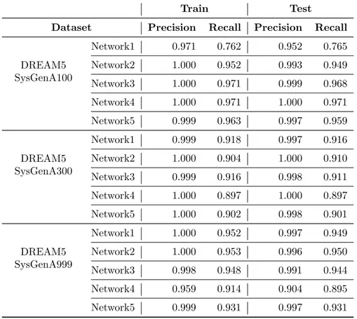
Statistical results, in terms of precision and recall, for both the training and the test instances are obtained considering, for each of the 15 datasets, the median over the 30 independent runs that were performed. We preferred the median over the average for its higher robustness to outliers. Table 1 summarizes all the results we obtained. As one can notice, the proposed system can achieve a good classifi-cation performance on both training and test instances, hence showing that it produces robust classifiers. In more in detail, all the median values of precision and recall obtained on the 15 networks are higher than 0.89 (except for the first network which has values around 0.76 for the recall). The overall median values on all networks computed in the training phase are 1 for the precision and 0.931 for the recall. On unseen instances (i.e. test phase) the values are 0.997 for the precision and 0.916 for the recall. A graphic presentation of the results achieved on all 30 runs on the 15 datasets is shown as a scatter plot in Figure 5, in which the area from 0.5 to 1 for both axes is shown. Red dots show the results obtained on the training sets, while light blue dots show
8 9 10 11 12 13 14 15 16 17 18 19 20 21 22 23 24 25 26 27 28 29 30 31 32 33 34 35 36 37 38 39 40 41 42 43 44 45 46 47 48 49 50 51 52 53 54 55 56 57
those obtained on the test sets.
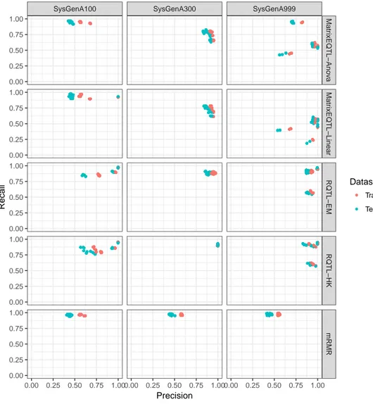
To better understand the improvements stemming from combining the predictions of the 5 tools/variants, we computed the precision and recall values for each of them on the 30 independent runs on the 15 datasets. To identify the SNP-gene pairs predicted as positive by each tool/variant, we adopted as a threshold to split the two classes the default values of each tool as suggested in the corresponding paper: mRMR scores higher than 0, p-values of MatrixEQTL (both linear and ANOVA) lower than 0.05, and R/qtl scores (both EM and HK) higher than 2. By reporting the precision and recall values on each independent run of each dataset, one may observe in Figure 3 that the results are quite different and, in some cases, not so good. These scatter plots show for the 3 DREAM5 sample sizes (on the columns) and for each tested tool/variant (on the rows) the precision and recall values achieved on the 30 independent runs for each of the 5 networks on both the training and test sets. Note that while MatrixEQTL and R/qtl reveal a similar trend on the networks with more samples (SysGenA300 and SysGenA999), mRMR has a very low recall and also a precision often under 0.5. Moreover, as expected, the results achieved on the training instances are better than those obtained for the unseen ones (test instances).
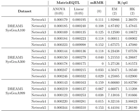
To quantify the improvement in the proposed system’s perfor-mance, we decided to apply our LMT system to each tool/variant separately. The aim of this analysis was to determine the best thresh-old for each tool/variant on every run of the tested datasets. The values of the computed thresholds reported in Table 2 differ in each
8 9 10 11 12 13 14 15 16 17 18 19 20 21 22 23 24 25 26 27 28 29 30 31 32 33 34 35 36 37 38 39 40 41 42 43 44 45 46 47 48 49 50 51 52 53 54 55 56 57
dataset, highlighting the fact that it is hard to find default values with-out considering the specific problem. The results shown in Figure 4 show a significant improvement in both precision and recall in almost all tested tools/variants, emphasizing the importance of the choice of the thresholds. In fact, although for each tool the authors suggest the ideal threshold value(s), each dataset varies from the others and so it is important to select the threshold values accordingly.
From this point of view, our method not only exploits the infor-mation provided by the different tools to achieve a better prediction, but is unconstrained by the particular threshold values. Moreover, these results show the the proposed method’s suitability for address-ing the problem under scrutiny: in particular, in the vast majority of datasets, the training and test performance are comparable. Hence, the method can not only extract a model of the data that produces a good classification of the training instances, but it also shows a good generalization ability.
This is also supported by the experimental analysis we performed on a real case study, consisting of a dataset of miRNA expression of 30 C. elegans recombinant in-bred lines [Kel (2016)]. These lines were obtained from the crosses between two different C. elegans strains: the
N2 wild-type ancestral worms and the wild CB4856 nematodes [Hodgkin and Doniach (1997)], isolated from Hawaii (HW). All individuals were genotyped across
1455 SNP markers [Rockman (2010)], while the miRNA expression profiles were estimated using the small RNA sequencing technology of Illumina [Kel (2016)].
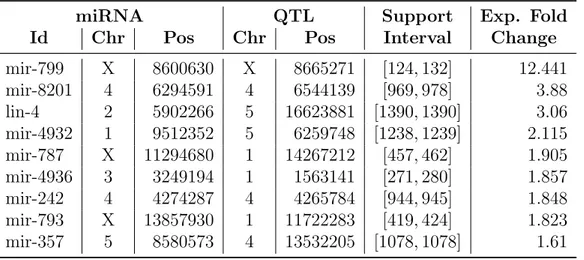
Table 3 gives an overview of the experimentally validated eQTL
8 9 10 11 12 13 14 15 16 17 18 19 20 21 22 23 24 25 26 27 28 29 30 31 32 33 34 35 36 37 38 39 40 41 42 43 44 45 46 47 48 49 50 51 52 53 54 55 56 57
results, which were all found by the proposed machine learning ap-proach. These predictions, concerning novel putative eQTLs, originate from the comparison between the HW and N2 strains of C. elegans and were experimentally validated. To this end, the effective miRNA differential expression was quantified on the 16 RILs that were most representative of the original set of 30, by using a Rotor Gene Real-Time PCR System (Qiagen) with Sybr Green miRNA assays (Qiagen) in accordance with the manufacturer’s instructions.
The predictions reported in Table 3 are experimentally confirmed, since the identified fold change supports our results considering the widely adopted 1.5 threshold. Moreover, as discussed in [Kel (2016)], none of the tools considered in our integration approach was able alone to predict all these eQTLs, while using our integration approach all the validated eQTLs are correctly predicted. This proves the superior performance of our machine learning approach, and that this method is generally applicable also to real datasets. We would like to point out that although our machine learning approach bases its classification process on a function, its value can not be used to score the predictions since it does not correspond to a quality measure. For this reason we only classified the instances and verified that the experimentally validated ones were correctly predicted.
4
Conclusions
In this work, we proposed a supervised learning approach to integrate eQTL predictions provided by different tools. In particular, we
com-8 9 10 11 12 13 14 15 16 17 18 19 20 21 22 23 24 25 26 27 28 29 30 31 32 33 34 35 36 37 38 39 40 41 42 43 44 45 46 47 48 49 50 51 52 53 54 55 56 57
bined two approaches, linear models and tree induction methods, that are very popular in the data mining community for solving a super-vised learning problem.
Linear model approaches fit a simple (linear) model to the data, with this process being quite stable, resulting in low variance, but potentially high bias. Tree induction methods exhibit low bias but often high variance: they search a less restricted space of models, allowing it to capture nonlinear patterns in the data, but making it less stable and prone to overfitting. Not surprisingly, neither method is generally superior. Much work has been done to combine these two schemes into model trees, namely, trees containing linear regression functions on the leaves. Hence, if only little and/or noisy data are available model trees rely on simple regression models, while if there are enough data more complex tree structures are used.
Moreover, since real SNP-gene interactions correspond to a small fraction of all the possible combinations (∼ 0.2%), another critical problem addressed in this work is that the set of elements of a spe-cific class (positive results) is very small relative to the overall dataset (whole predictions). The predictions obtained with most of the clas-sifiers are influenced by the fact that the classes are not equally bal-anced. These approaches assume that all misclassification errors come at equal cost, while in several applications this assumption may not be true. To avoid this problem, we used a method called One Side Se-lection, which undersamples the class containing the highest number of elements.
The results obtained using our Logistic Model Trees on the DREAM5
8 9 10 11 12 13 14 15 16 17 18 19 20 21 22 23 24 25 26 27 28 29 30 31 32 33 34 35 36 37 38 39 40 41 42 43 44 45 46 47 48 49 50 51 52 53 54 55 56 57
challenge datasets are encouraging, showing we are always able to achieve better results than the original tools. This is achieved by combining the predictions obtained by each tool, but also by com-puting the “best” threshold values for each of them on the analyzed dataset. For this reason, we plan to extend our integrative approach to other software to further reduce the number of false positive results, as well as to apply the presented machine learning technique to other datasets to assess its power on real case studies.
Acknowledgments
This work has been supported by the Italian Ministry of Education and Research (MIUR) through the Flagship (PB05) InterOmics and HIRMA (RBAP11YS7K), and by the FP7-HEALTH through the Eu-ropean MIMOMICS projects (no. 305280).
8 9 10 11 12 13 14 15 16 17 18 19 20 21 22 23 24 25 26 27 28 29 30 31 32 33 34 35 36 37 38 39 40 41 42 43 44 45 46 47 48 49 50 51 52 53 54 55 56 57
References
[Abecasis (2002)] Abecasis, G.R., Cherny, S.S., Cookson, W.O., et al. 2002. Merlinrapid analysis of dense genetic maps using sparse gene flow trees. Nature Genetics, 30(1), 97–101.
[Ackermann (2012)] Ackermann, M., Clment-Ziza, M., Michaelson, J.J., et al. 2012. Teamwork: improved eQTL mapping using com-binations of machine learning methods. PloS One, 7(7), e40916. [Appice (2008)] Appice, A., Ceci, M., Malerba, D., et al. 2008. Step-wise induction of logistic model trees. Foundations of Intelligent Systems, 68–77.
[Beretta (2016)] Beretta, S., Castelli, M., Gonalves, I., et al. 2016. Combining Bayesian Approaches and Evolutionary Techniques for the Inference of Breast Cancer Networks, 217–224. In Proceed-ings of the 8th International Joint Conference on Computational Intelligence (IJCCI). SciTePress.
[Beretta (2017)] Beretta, S., Maj, C., and Merelli, I. 2017. Rank miRNA: a web tool for identifying polymorphisms altering miRNA target sites, 1125–1134. In Proceedings of International Conference on Computational Science (ICCS). Procedia Com-puter Science.
[Bishop (2006)] Bishop, C.M. 2006. Pattern Recognition and Machine Learning. Springer-Verlag, New York.
[Broman (2003)] Broman, K.W., Wu, H., Sen, ´S., et al. 2003. R/qtl: QTL mapping in experimental crosses. Bioinformatics, 19(7), 889–890. 8 9 10 11 12 13 14 15 16 17 18 19 20 21 22 23 24 25 26 27 28 29 30 31 32 33 34 35 36 37 38 39 40 41 42 43 44 45 46 47 48 49 50 51 52 53 54 55 56 57
[Caruana and Mizil (2006)] Caruana, R., and Niculescu-Mizil, A. 2006. An empirical comparison of supervised learn-ing algorithms, 161–168. In Proceedlearn-ings of the 23rd international conference on Machine learning. ACM, New York.
[Duggal (2014)] Duggal, G., Wang, H., and Kingsford, C. 2014. Higher-order chromatin domains link eQTLs with the expression of far-away genes. Nucleic Acids Research, 42(1), 87–96.
[Friedman (2000)] Friedman, J., Hastie, T., Tibshirani, R. et al. 2000. Additive logistic regression: a statistical view of boosting (with discussion and a rejoinder by the authors). The annals of statis-tics, 28(2), 337–407.
[Ganganwar (2012)] Ganganwar, V. 2012. An overview of classifica-tion algorithms for imbalanced datasets. Internaclassifica-tional Journal of Emerging Technology and Advanced Engineering, 2(4), 42–47. [Guo (2008)] Guo, X., Yin, Y., Dong, C., Yang, et al. 2008. On the class imbalance problem, 192–201. In Guo, M., Zhao, L., and Wang L. eds. Natural Computation, ICNC’08. Fourth Interna-tional Conference on. IEEE.
[Hall (2009)] Hall, M., Frank, E. Holmes, G. et al. 2009. The WEKA data mining software: an update. ACM SIGKDD Explorations Newsletter, 11(1), 10–18.
[Harrell Jr (2015)] Harrell Jr, F.E. 2015. Regression Modeling Strate-gies: With Applications to Linear Models, Logistic and Ordinal Regression, and Survival Analysis. Springer, New-York.
8 9 10 11 12 13 14 15 16 17 18 19 20 21 22 23 24 25 26 27 28 29 30 31 32 33 34 35 36 37 38 39 40 41 42 43 44 45 46 47 48 49 50 51 52 53 54 55 56 57
[Hart (1968)] Hart, P. 1968. The condensed nearest neighbor rule (Corresp.). IEEE Transactions on Information Theory, 14(3), 515–51.
[Hastie (2009)] Hastie, T., Tibshirani, R., and Friedman, J. 2009. Overview of Supervised Learning. Springer-Verlag, New York. [Hodgkin and Doniach (1997)] Hodgkin, J., and Doniach, T. 1997.
Natural variation and copulatory plug formation in Caenorhab-ditis elegans. Genetics, 146(1), 149–164.
[Hoggart (2008)] Hoggart, C.J., Whittaker, J.C., De Iorio, M., et al. 2008. Simultaneous analysis of all SNPs in genome-wide and re-sequencing association studies. PLoS Genetics, 4(7), e1000130. [Hosmer Jr (2013)] Hosmer Jr, D.W., Lemeshow, S., and Sturdivant,
R.X. 2013. Applied Logistic Legression. John Wiley & Sons. [Huang and Cai (2013)] Huang, T., and Cai, Y.D. 2013. An
information-theoretic machine learning approach to expression QTL analysis. PloS One, 8(6), e67899.
[Japkowicz and Stephen (2002)] Japkowicz, N., and Stephen, S. 2002. The class imbalance problem: A systematic study. Intelligent Data Analysis, 5(6), 429–449.
[Kao (1999)] Kao, C.H., Zeng, Z.B., Teasdale, R.D. 1999. Multiple interval mapping for quantitative trait loci. Genetics, 152(3), 1203–1216.
[Kel (2016)] Kel, I., Chang, Z., Galluccio, N., et al. 2016. SPIRE, a modular pipeline for eQTL analysis of RNA-Seq data, reveals a
8 9 10 11 12 13 14 15 16 17 18 19 20 21 22 23 24 25 26 27 28 29 30 31 32 33 34 35 36 37 38 39 40 41 42 43 44 45 46 47 48 49 50 51 52 53 54 55 56 57
regulatory hotspot controlling miRNA expression in C. elegans. Molecular BioSystems, 12(11), 3447–3458.
[Kubat and Matwin (1997)] Kubat, M., and Matwin, S. 1997. Ad-dressing the curse of imbalanced training sets: one-sided selec-tion, 179–186. In Fisher, D.M. eds. International Conference on Machine Learning, Morgan Kaufmann, Burlington.
[Landwehr (2005)] Landwehr, N., Hall, M., Frank, E. 2005. Logistic model trees. Machine Learning, 59(1-2), 161–205.
[Laurikkala (2001)] Laurikkala, J. 2001. Improving identification of difficult small classes by balancing class distribution. Artificial Intelligence in Medicine, 63–66.
[Lee (2008)] Lee, S.H., van der Werf, J.H., Hayes, B.J., et al. 2008. Predicting unobserved phenotypes for complex traits from whole-genome SNP data. PLoS Genetics, 4(10), e1000231.
[Leek and Storey (2007)] Leek, J.T., and Storey, J.D. 2007. Captur-ing heterogeneity in gene expression studies by surrogate variable analysis. PLoS Genetics, 3(9), e161.
[Loh (2011)] Loh, W.Y. 2011. Classification and regression trees. Wi-ley Interdisciplinary Reviews: Data Mining and Knowledge Dis-covery, 1(1), 14–23.
[Merelli (2013)] Merelli, I., Calabria, A., Cozzi, P., et al. 2013. SNPranker 2.0: a gene-centric data mining tool for diseases asso-ciated SNP prioritization in GWAS. BMC Bioinformatics, 14(1), S9. 8 9 10 11 12 13 14 15 16 17 18 19 20 21 22 23 24 25 26 27 28 29 30 31 32 33 34 35 36 37 38 39 40 41 42 43 44 45 46 47 48 49 50 51 52 53 54 55 56 57
[Merelli (2015)] Merelli, I., Tordini, F., Drocco, M., et al. 2015. In-tegrating multi-omic features exploiting Chromosome Conforma-tion Capture data. Frontiers in Genetics, 40, 1664–8021.
[Michaelson (2010)] Michaelson, J.J., Alberts, R., Schughart, K., et al. 2010. Data-driven assessment of eQTL mapping methods. BMC Genomics, 11(1), 502.
[Nguyen (2009)] Nguyen, G.H., Bouzerdoum, A., Phung, S. 2009. Learning pattern classification tasks with imbalanced data sets, 193–208. In Yin, P. eds. Pattern recognition, Vukovar, Croatia: In-Teh.
[Rockman (2010)] Rockman, M.V., Skrovanek, S.S., and Kruglyak, L. 2010. Selection at linked sites shapes heritable phenotypic variation in C. elegans. Science, 330(6002), 372–376.
[Shabalin (2012)] Shabalin, A.A. 2012. Matrix eQTL: ultra fast eQTL analysis via large matrix operations. Bioinformatics, 28(10):1353–1358.
[Servin and Stephens (2007)] Servin, B., and Stephens, M. 2007. Imputation-based analysis of association studies: candidate re-gions and quantitative traits. PLoS Genetics, 3(7), e114.
[Sumner (2005)] Sumner, M., Frank, E., and Hall, M. 2005. Speeding up logistic model tree induction, 675–683. In A. Jorge et al. eds. Knowledge Discovery in Databases: PKDD 2005. Springer-Verlag, Berlin.
[Tomek (1976)] Tomek, I. 1976. Two modifications of CNN. IEEE Trans. Systems, Man and Cybernetics, 6, 769–772.
8 9 10 11 12 13 14 15 16 17 18 19 20 21 22 23 24 25 26 27 28 29 30 31 32 33 34 35 36 37 38 39 40 41 42 43 44 45 46 47 48 49 50 51 52 53 54 55 56 57
[Witten (2016)] Witten, I.H ., Eibe, F., Hall, M.A. et al. 2016. Data Mining: Practical Machine Learning Tools and Techniques. Mor-gan Kaufmann, Burlington.
[Wright (2012)] Wright, F.A., Shabalin, A.A., and Rusyn, I. 2012. Computational tools for discovery and interpretation of expres-sion quantitative trait loci. Pharmacogenomics, 13(3), 343–352. [Zeng (1993)] Zeng, Z.B. 1993. Theoretical basis for separation of
multiple linked gene effects in mapping quantitative trait loci. Proceedings of the National Academy of Sciences, 90(23), 10972– 10976. 8 9 10 11 12 13 14 15 16 17 18 19 20 21 22 23 24 25 26 27 28 29 30 31 32 33 34 35 36 37 38 39 40 41 42 43 44 45 46 47 48 49 50 51 52 53 54 55 56 57
Table 1: Classification performance on the training and test instances for datasets considered. Averages values of Precision and Recall over the 30 independent runs are reported for each of the 15 datasets.
Train Test
Dataset Precision Recall Precision Recall
DREAM5 SysGenA100 Network1 0.971 0.762 0.952 0.765 Network2 1.000 0.952 0.993 0.949 Network3 1.000 0.971 0.999 0.968 Network4 1.000 0.971 1.000 0.971 Network5 0.999 0.963 0.997 0.959 DREAM5 SysGenA300 Network1 0.999 0.918 0.997 0.916 Network2 1.000 0.904 1.000 0.910 Network3 0.999 0.916 0.998 0.911 Network4 1.000 0.897 1.000 0.897 Network5 1.000 0.902 0.998 0.901 DREAM5 SysGenA999 Network1 1.000 0.952 0.997 0.949 Network2 1.000 0.953 0.996 0.950 Network3 0.998 0.948 0.991 0.944 Network4 0.959 0.914 0.904 0.895 Network5 0.999 0.931 0.997 0.931 8 9 10 11 12 13 14 15 16 17 18 19 20 21 22 23 24 25 26 27 28 29 30 31 32 33 34 35 36 37 38 39 40 41 42 43 44 45 46 47 48 49 50 51 52 53 54 55 56 57
Table 2: Threshold values obtained with the machine learning classifier on each single tool. For each dataset we reported the threshold computed with the LMT classifier by considering the predictions of each tool/variant in-dependently. Default values for each prediction tool/variant are shown in parentheses. MatrixEQTL mRMR R/qtl Dataset ANOVA (0.05) Linear (0.05) (0) EM (2) HK (2) DREAM5 SysGenA100 Network1 0.000179 0.000195 0.111 1.92866 2.36070 Network2 0.000185 0.000240 0.108 4.87492 5.47845 Network3 0.000169 0.000135 0.125 0.12500 0.10672 Network4 0.000184 0.000223 0.118 0.00011 0.08902 Network5 0.000223 0.009998 0.152 1.67575 1.47080 DREAM5 SysGenA300 Network1 0.000144 0.000136 0.118 6.23438 7.07576 Network2 0.000150 0.000279 0.040 5.21553 6.20687 Network3 0.000178 0.000175 0 5.27126 5.81573 Network4 0.000247 0.000215 0.033 4.50471 5.16540 Network5 0.000246 0.000332 0.029 4.25885 0.02900 DREAM5 SysGenA999 Network1 0.000143 0.000163 0.159 8.66660 10.83790 Network2 0.000219 0.000137 0.067 4.66071 5.11208 Network3 0.000123 0.000253 0.038 7.13816 7.81666 Network4 0.000220 0.000281 0.015 8.32116 3.88823 Network5 0.000344 0.000310 0.153 6.44104 7.26180 8 9 10 11 12 13 14 15 16 17 18 19 20 21 22 23 24 25 26 27 28 29 30 31 32 33 34 35 36 37 38 39 40 41 42 43 44 45 46 47 48 49 50 51 52 53 54 55 56 57
Table 3: Experimentally validated eQTL predictions for the C. elegans dataset. For each prediction miRNA and QTL coordinates are reported, and also the support interval of the miRNA. Predictions are sorted accord-ing to the expression fold change calculated usaccord-ing ddCT values on the results of qPCR validation.
miRNA QTL Support Exp. Fold
Id Chr Pos Chr Pos Interval Change
mir-799 X 8600630 X 8665271 [124, 132] 12.441 mir-8201 4 6294591 4 6544139 [969, 978] 3.88 lin-4 2 5902266 5 16623881 [1390, 1390] 3.06 mir-4932 1 9512352 5 6259748 [1238, 1239] 2.115 mir-787 X 11294680 1 14267212 [457, 462] 1.905 mir-4936 3 3249194 1 1563141 [271, 280] 1.857 mir-242 4 4274287 4 4265784 [944, 945] 1.848 mir-793 X 13857930 1 11722283 [419, 424] 1.823 mir-357 5 8580573 4 13532205 [1078, 1078] 1.61 8 9 10 11 12 13 14 15 16 17 18 19 20 21 22 23 24 25 26 27 28 29 30 31 32 33 34 35 36 37 38 39 40 41 42 43 44 45 46 47 48 49 50 51 52 53 54 55 56 57
Figure 1: Example of the distribution of instances in a two-class dataset: stars denote instances in the minority class, circles denote instances in the majority class. 8 9 10 11 12 13 14 15 16 17 18 19 20 21 22 23 24 25 26 27 28 29 30 31 32 33 34 35 36 37 38 39 40 41 42 43 44 45 46 47 48 49 50 51 52 53 54 55 56 57
Figure 2: Graphical presentation of the LMT learning algorithm. 8 9 10 11 12 13 14 15 16 17 18 19 20 21 22 23 24 25 26 27 28 29 30 31 32 33 34 35 36 37 38 39 40 41 42 43 44 45 46 47 48 49 50 51 52 53 54 55 56 57
SysGenA100 SysGenA300 SysGenA999 Matr ixEQTL−Ano v a Matr ixEQTL−Linear RQTL−EM RQTL−HK mRMR 0.00 0.25 0.50 0.75 1.000.00 0.25 0.50 0.75 1.000.00 0.25 0.50 0.75 1.00 0.00 0.25 0.50 0.75 1.00 0.00 0.25 0.50 0.75 1.00 0.00 0.25 0.50 0.75 1.00 0.00 0.25 0.50 0.75 1.00 0.00 0.25 0.50 0.75 1.00 Precision Recall Dataset Training Test
Figure 3: Scatter plots showing the precision and recall achieved by each considered tool/variant with suggested threshold values (rows) on the 30 in-dependent runs of the 15 DREAM5 datasets, split by sample size (columns). Colors highlight the two sets: Training (red) and Test (light blue).
8 9 10 11 12 13 14 15 16 17 18 19 20 21 22 23 24 25 26 27 28 29 30 31 32 33 34 35 36 37 38 39 40 41 42 43 44 45 46 47 48 49 50 51 52 53 54 55 56 57
SysGenA100 SysGenA300 SysGenA999 Matr ixEQTL−Ano v a Matr ixEQTL−Linear RQTL−EM RQTL−HK mRMR 0.00 0.25 0.50 0.75 1.000.00 0.25 0.50 0.75 1.000.00 0.25 0.50 0.75 1.00 0.00 0.25 0.50 0.75 1.00 0.00 0.25 0.50 0.75 1.00 0.00 0.25 0.50 0.75 1.00 0.00 0.25 0.50 0.75 1.00 0.00 0.25 0.50 0.75 1.00 Precision Recall Dataset Training Test
Figure 4: Scatter plots showing the precision and recall achieved by each considered tool/variant with optimal threshold values (rows) on the 30 inde-pendent runs of the 15 DREAM5 datasets, split by sample size (columns). Colors highlight the two sets: Training (red) and Test (light blue).
8 9 10 11 12 13 14 15 16 17 18 19 20 21 22 23 24 25 26 27 28 29 30 31 32 33 34 35 36 37 38 39 40 41 42 43 44 45 46 47 48 49 50 51 52 53 54 55 56 57
SysGenA999 SysGenA300 SysGenA100 0.5 0.6 0.7 0.8 0.9 1.0 0.5 0.6 0.7 0.8 0.9 1.0 0.5 0.6 0.7 0.8 0.9 1.0 0.5 0.6 0.7 0.8 0.9 1.0 Precision Recall Dataset Training Test
Figure 5: Scatter plots showing the Precision and Recall achieved by our approach on the 30 independent runs of the 15 DREAM5 datasets, split by sample size (rows), in both Training (red) and Test (light blue) sets. Here, only the area from 0.5 to 1 on both axes is shown.
8 9 10 11 12 13 14 15 16 17 18 19 20 21 22 23 24 25 26 27 28 29 30 31 32 33 34 35 36 37 38 39 40 41 42 43 44 45 46 47 48 49 50 51 52 53 54 55 56 57