Economic Structure and Growth

ECONOMIC STRUCTURE AND GROWTH

Dissertation

Master in Economics

Supervised by

Pedro Rui Mazeda Gil Óscar João Atanázio Afonso

Abstract

The purpose of this study is to analyse the impact of the economic structure on economic growth, a question that brings together economic growth and development economics. In particular, we want to assess if a high specialization in some sectors, as opposed to a more diversified economy, influences the rate of growth of the economy. Our results indicate that, although not uniform between countries from different regions and income levels, economic structure plays a role in the explanation of economic growth.

JEL codes: O10, O40, 050

Keywords: Economic Growth, Economic Structure, Specialization, Diversification

Resumo

O objectivo deste estudo passa por analisar o impacto da estrutura da economia no crescimento económico, uma questão transversal ao crescimento e ao desenvolvimento económico. Em particular, queremos avaliar se uma maior especialização em determinados sectores, em comparação com uma economia mais diversificada, influencia a taxa de crescimento da economia. Os nossos resultados indicam que, embora não uniforme entre países de regiões e níveis de rendimento diferentes, a estrutura da economia é importante para explicar o crescimento económico.

Classificação JEL: O10, 040, 050

Palavras-chave: Crescimento Económico, Estrutura da Economia, Especialização, Diversificação

Index of Contents

1. Introduction ………...……….…….. 1

2. Literature Review ……….……. 3

2.1 The Classic View ……….. 3

2.2 Growth and Development ………...……… 3

2.3 The emergence of “product space” ……….….. 6

2.4 Structure and Growth at a Regional Level ……….…...……. 7

3. The Economic Structure ………..……..……….. 10

3.1 Definition ……….. 10

3.2 Measurement ………. 11

3.2.1 Sector’s size dimensions ……….…………. 11

3.2.2 Indicators of Specialization/Diversification ………...…….………. 12

3.2.3 The Level of Aggregation ………...………. 15

3.3 Data ……….…….. 16

4. Growth Accounting Model ………...……….. 19

4.1 Estimation Procedure ……… 20

4.1.1 Model Setup ………..……….. 20

4.1.1.1 Specification for labour efficiency ………...…….. 22

4.1.1.2 Specification for capital efficiency ……… 23

4.2 Data ……….….. 24 4.3 Panel Estimation ………....……… 26 4.4 General Results ……….. 27 4.5 Extensions ……….……… 30 4.5.1 Geographic Groups ……… 30 4.5.2 Income ………..……….. 32 4.5.3 Export Clubs ……….….. 33 4.6 Robustness Analysis ………...…… 35 5. Economic Complexity ………...…………. 37 5.1 Results ……….……….. 37 6. Conclusions ………..……….. 39 7. References ………. 41

Index of Tables

Table 3.1 – Summary statistics for the specialization/diversification indices …………... 16 Table 3.2 – Correlation matrices for the specialization/diversification indices ……….... 17 Table 4.1 – Panel data estimation of the relationship between economic structure and

wage growth (Main Results) ……… 27

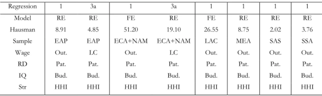
Table 4.2 – Panel data estimation of the relationship between economic structure and

wage growth (by Geographic Groups) ………. 30

Table 4.3 – Panel data estimation of the relationship between economic structure and

wage growth (by Income Levels) ………. 32

Table 4.4 – Panel data estimation of the relationship between economic structure and

wage growth (by Export Clubs) ………... 33

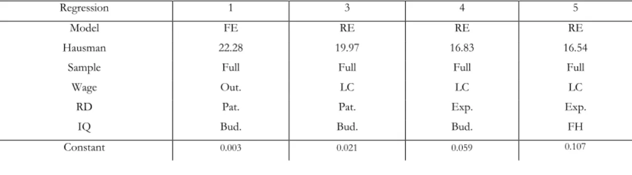
Table 4.5 – Panel data estimation of the relationship between economic structure and

wage growth (Robustness Analysis for EU+US) ………. 35

Table 5.1 – Panel data estimation of the relationship between economic complexity and

1. Introduction

Economies from all over the world are all different. Some countries have a specialization in the production of a specific good, while others produce a diverse range of products. Some countries face continuous growth while others are stagnated or show an unstable pattern. It is conceivable that these two dimensions – economic structure and economic growth – are related. Therefore, the purpose of this study is to analyse whether a high specialization in some sectors, as opposed to a more diversified economy, influences the rate of growth of the economy.

The causes of economic growth had intrigued philosophers and political thinkers since the beginning of times. It can be argued that this question is on the origin of economics as a science. Several possible explanations have been proposed, especially after Solow (1956) and his growth theory based on the accumulation of physical inputs, such as labour and capital (including land), and on technological progress. Once the “technological progress” cannot be observed, this factor can capture the effect of several elements, where we can include the structure of the economy. This theoretical framework, associated with the fact that nowadays several countries (mainly developing countries) are highly dependent on the performance of natural resource exploration (natural gas, oil and hard minerals), motivate this study that will try to answer the general question “Why is diversification so important?”

As the above question is, however, still quite general, we defined three more specific questions which will allow us to reach a conclusion: What’s the impact of the structure of the economy on economic growth? Does this impact depend on the dominant sector? Does the economic structure effect depend on the sectoral branches within the economy?

In order to do that, we will develop a model, formalizing a general relationship between the two referred concepts (economic structure and economic growth), using a growth-accounting framework. We also analysed diversities across countries from diverse regions and having different income levels. A deeper analysis of some particular sectors was developed in order to test if the presented results are sensitive to the sector considered. Lastly, we analysed if the economic complexity impacts on economic growth.

Our results indicate that, although not uniform between countries from different regions and income levels, economic structure plays a role in the explanation of economic growth.

Several studies tried to explain the relationship between these two dimensions. The present paper, however, pursues a slightly different point of view. While other studies confront the complexity of the economy or the sectoral composition of national production with economic growth, this research aims to understand the possible impact of the structure of the economy on economic growth. This study could, also, be helpful to define growth promoting guidelines, especially in developing countries.

The remainder of the study is organized as follows. In the following section, we review the literature that analyses the relationship between economic structure and economic growth. In the third section, we explain our approach to the measurement of the economic structure and the data used. In the fourth section, we describe the empirical model estimated, reveal the general results obtained and explore differences between regions, income levels and export clubs. Section 5 goes further and includes economic complexity as a possible explanation for growth. The last section concludes.

2. Literature review

Although our objective is to study the impact of economic structure on economic growth, the lack of studies addressing our question leads us to refer similar works that do not use the exact approach we want to pursue. We also choose to refer studies with “level effects” although our interest lies in the “growth effects”. Both empirical and theoretical literature was considered. The available empirical evidence on the relationship between economic structure and economic growth is not conclusive. Although the majority of studies within this topic are employed on a regional level, analysis differs on time or area under study, the measures of diversification/specialization used, the industrial taxonomy considered and even on the methods applied.

2.1 The Classic View

The causes of economic growth had intrigued philosophers and political thinkers since the beginning of times. It can be argued that this question is on the origin of economics as a science. Indeed, since Adam Smith (1776) and his theory of specialization, several authors explored this issue. However, we needed to wait almost two hundred years before the Solow growth model. This model changed the paradigm and provided a decisive impulse to the study of economic growth. Since then and up to now, the study of economic growth has seen a continuous and solid evolution.

Solow (1956) proposes a growth theory based on the accumulation of physical inputs, such as labour and capital (including land), and on technological progress. Once the “technological progress” cannot be observed, this factor can capture the effect of several elements – the well-known “Solow residual”. Many economists have tried to identify all the possible sources of growth, ever since.

2.2 Growth and Development

At a certain point, these studies began to consider the structure of the economy as a possible explanatory variable of economic growth. Lewis (1954), Rostow (1959), Chenery (1960, 1982), among others, studied structural transformation as the process of reallocation of production structure that accompanies the process of economic growth and Kuznets (1971) exploited the impact of changes in sectoral composition on economic growth. But

the idea of the structure of the economy impacting economic growth goes back to Young (1928). This author pointed to the relationships between the various industries1 _{in the}

economy as having impact on the growth pattern of the economy.

The majority of this studies converges to the idea of a two-way causality between economic growth and structural change. This is, during the development process, while economies move from agriculture and extractive industries to more sophisticated forms of manufacturing and services, the mechanics of growth and structural change interchange effects in a dynamic way.

Related to this older line of research, but focused on a much broader approach, Imbs and Wacziarg (2003) and Klinger and Lederman (2004) studied how the economic structure evolves with development. The first studied the evolution of sectoral concentration in relation to the level of per capita income for a wide range of industrial and developing countries. Using nonparametric methods, they found that the relationship between sectoral diversification and income follows a U-shaped pattern: countries first tend to diversify, but lately on the development process occurs the inverse and countries start specializing again. One possible explanation for this evolution can be found in the work of Klinger and Lederman (2004). They analyzed the evolution of export discoveries – new export products introduced – on the level of development by applying panel estimation models to data from 99 countries for various time periods. Although the discovery activity is just one of two channels for diversification to occur – being the other a more evenly production across all the existing sectors - the result suggests discovery to be an important element to understand the evolution of the economic structure with development. Discovery activity appears to follow an inverted U-curve in income: the number of new export products increases with income when countries are in development, on a later stage the discovery activity declines and countries start specializing again.

In the late 90’s a new approach appeared. This view tries to achieve simultaneously structural transformation and a balanced growth path, by constructing models where the continuous process of production and employment reallocation between sectors go hand in hand with the stable behaviour that characterizes the aggregate variables in a balanced growth path. Broadly speaking, this approach aims to gather the abovementioned Kuznets

facts with the well-known Kaldor facts2 _{in a single model. This literature divided into two}

branches, according to the considered driving force behind the structural transformation. Some authors, such as Echevarria (1997), Kongsamut et al. (2001) and Foelmi and Zweimüller (2008) believe that structural change occurs due to sectoral differences in income elasticities of demand. This “demand-side” explanation states that the marginal rate of substitution between different goods changes as an economy grows, decreasing the relative weight of necessities and increasing the share of luxury goods on total expenditures, a theory that it’s aligned with Engel’s law. Echevarria (1997) represents – to the best of our knowledge – the first attempt to reconcile the structural transformation within the usual growth models framework. This paper presents a dynamic general equilibrium model with different income elasticities for the three sectors considered – primaries, manufacturing and services. Kongsamut et al. (2001) developed a standard growth model; but, in contrast with Echevarria (1997), only required the real interest rate to remain constant over time – a generalized balanced growth path. Foelmi and Zweimüller (2008) proposed a different technique. In their model, new goods are continuously introduced into the economy. With a hierarchic utility function, the production of new goods increases while old industries disappear. Sectoral differences in income elasticities arise, leading to the structural change that affects economic growth.

Other authors, such as Ngai and Pissarides (2007) and Acemoglu and Guerrieri (2008) rely on the relative price change effect as the cause of structural change. This mechanism reflects differences in Total Factor Productivity (TFP) growth rates across sectors and is inspired by the seminal contribution of Baumol (1967), which explains the structural change as a result of a “supply-side” phenomenon. Baumol argues that the economy can be divided into two sectors – a “progressive” and a “non-progressive” sector. While the “progressive” sector exhibits technological progress, the “non-progressive” sector remains technologically unchanged over time. This “technological” explanation was the key mechanism besides the model of Ngai and Pissarides (2007), which considers TFP differences across sectors to be exogenous. Their results confirm Baumol’s claim about structural change: over time the labour force is channelled from the high to the low TFP activities. The same model, however, predicts a different pattern if we consider a finer sector decomposition. In this case, within the subsectors, there is an inverse flow with

2 _{Kaldor (1961) points out the stable behaviour of the growth rate of output, the capital-output ratio, the} share of capital income in GDP and the real interest rate, which are all approximately stationary over time. These “stylized facts” have been used ever since.

labour moving from low to high TFP goods. Acemoglu and Guerrieri (2008) pursued another explanation, although closer to that of Ngai and Pissarides (2007). Their two-sector general equilibrium model states that nonbalanced growth is based on differences in factor proportions (capital intensities) between sectors and capital deepening. As a result, there is an increase in the relative output of the more capital-intensive sector while there is a shift of capital and labour away from this sector.

Both mechanisms – income effects and relative price changes – are believed to account for structural transformation. Although the majority of studies within this framework usually apply one of them separately, some authors tried to explain the joint possibility of structural transformation and balanced growth path considering both effects at once. Bonatti and Felice (2007) extended the analysis of Echevarria (1997) and Kongsmaut et al. (2001) by allowing for endogenous growth and for relaxing the condition of equal TFP growth rate across sectors. Their two-sector endogenous growth model show under what circumstances on preferences Baumol’s claim occurs. Lately, Boppart (2014) presents structural change as a result both from income effects and substitution effects. Applying the model to the U.S. economy, concluded that both channels appear to have roughly the same importance explaining the observed structural change.

2.3 The emergence of “product space”

Lately emerged the concept of “product space” created by Hausmann et al. (2007). This concept was built on the idea of Hirschman (1958), who studied backwards and forward linkages across economic sectors and suggested that industrialization creates externalities that can promote economic growth. Within this framework, economic sectors are distributed accordingly with their linkages and the available capabilities in the country. The impact of economic structure on economic growth varies accordingly with the sectors in which the country is specialized, being some products associated with higher productivity levels than others. They conclude that “rich (poor) countries export products that tend to be exported by other rich (poor) countries” (p. 10) and, therefore, measures of economic complexity can predict future economic growth.

This new concept revolutionized the study of the economic structure and promoted further research on the impact of economic complexity on economic growth. Hidalgo and Hausmann (2009), Boschma et al. (2012), Felipe et al. (2012), and Ferrarini and

Scaramozzino (2016), using different approaches, all conclude that economic complexity affects economic growth.

The first concludes that countries tend to converge to the income associated with the products they produce. Thus, to promote growth, policymakers should generate conditions to increase production complexity. Since some products have associated a higher spillover effect than others, ventures to produce more complex goods – more linked within the product space – allow accumulating new capabilities, essential to produce even more complex products and, thus, expand the country’s set of abilities.

Both Boschma et al. (2012) and Felipe et al. (2012) applied the methodology proposed by Hidalgo and Hausmann. Felipe et al. (2012), studying 124 countries and 5107 products, found that the complexity of the exports changes with income. The exports of more (less) complex products increase (decrease) with the level of development of the country. They confirmed the theories of Hidalgo and Hausmann (2009), arguing to the need of “policies that foster the accumulation of capabilities and promote the development of new more complex products, i.e., diversify” (p. 52). Boschma et al. (2012), studying Spanish regions economic performance between 1988 and 2008, also conclude that territories should diversify, but “into industries that are related to the existing set of industries” (p. 2), to allow knowledge spillovers to occur.

Ferrarini and Scaramozzino (2016) follow the same idea studying both growth and level effects of production complexity on economic growth. Their endogenous growth model considers that production complexity plays a dual role: can promote human capital accumulation –following Lucas’ human capital theory (Lucas, 1988) –, and increase the risk of production failure – consistent with Kremer’s O-ring theory (Kremer, 1993). They conclude that “increased complexity has an ambiguous effect on the level of output, but positively impacts economic growth by enhancing human capital formation” (p. 17).

2.4 Structure and Growth at a Regional Level

Another trend in the literature, based on the pioneering work of Chinitz (1961), tries to explain the relationship between economic structure and growth at a regional level. We consider this literature as relevant to our study and choose to refer to it even though the different geographic scale makes difficult for direct comparisons.

This literature usually studies how economic structure relates to innovation and, therefore, with economic growth. There are two competing theories to explain this relationship. Jacobs (1969) stated that innovation occurs from the spillover effect through different sectors or inter-sectoral spillovers. A more diversified economy promotes the interaction between industries, which allows a “cross-fertilization” of ideas and fosters the appearance of new products and technologies. On the opposite side, Marshall (1890) considers that intra-sectoral spillovers, or spillovers occurring within a sector, are the driving force behind regional economic growth. It is assumed that specialization on a given sector leads to productivity gains through process innovation.

Empirical studies tried to understand which of the effects, spillovers occurring from diversification or specialization, is stronger. While Wagner and Deller (1998), studying the 50 US states for the period 1969-1992, found a positive impact of diversity on growth, Attaran (1986), comparing industrial diversity with economic performance – measured either by unemployment and per capita income -, in US areas (50 states and the District of Columbia) for the ten-year period 1972-1981, discovered an unexpected negative effect of diversity on per capita income growth at the region level. The results also reveal a negative but very weakly correlation between diversity and unemployment growth. A similar result was obtained by Glaeser et al. (1992) considering data from 170 American cities for the period 1956-1987. They found specialization to be negatively correlated with employment growth, in opposition to diversification which appears to have a positive effect, consistent with the theories of Jacobs. Besides this, Izraeli and Murphy (2003), applying panel data techniques – which allow controlling for unobserved individual heterogeneity - with a sample of 17 US states spanning a 38-year period (1960-1997) do not find any significant impact of diversity on per capita income growth.

Two other studies were conducted for the case of the Netherlands. Van Stel and Nieuwenhuijsen (2004), studying the impact of knowledge spillovers on economic growth, found a positive effect of diversity on value-added growth. Frenken et al. (2007), analyzing the effect of variety on regional economic growth, found that related variety – within sectors – enhances economic growth, while unrelated variety – between sectors (diversification) – has a negative effect on unemployment growth. Both analysis used data from Dutch regions at the NUTS 3 level.

It should also be stressed another theory that relates economic structure with stability and, therefore, with economic growth. The literature pioneered by McLaughlin (1930), Hoover (1948) and Nourse (1968) argue that diversity promotes economic stability.

A more diversified economy is believed to become less responsive to business fluctuations than a more specialized one. Diversification allows the stability of employment and income through compensating seasonal and cyclical fluctuations across a wide range of industries. On the long-run, as stated by Hoover (1948), “diversification affords some insurance against the total collapse of the economic life” (p. 288). The employment of complimentary labour groups – contrary to just one or few groups of workers employed in the case of more specialized economies – makes it easier to replace declining industries and, therefore, allows to protect against secular and structural changes. Pasinetti (1993) goes further and analyses this impact through employment, considering that without diversification an economy will suffer from structural unemployment and, consequently, low economic growth.

This theory also argues that specialization cannot protect the economy from external shocks in demand (Attaran, 1986; Izraeli and Murphy, 2001). On contrary, the process of diversification increases the degree of risk spreading that an economy can achieve (Acemoglu and Zilibotti, 1997). With diversification, the effect of sector-specific shocks is mitigated through a broader portfolio of economic sectors, which fosters investment and the development of financial markets. This will ultimately promote economic growth. Frenken et al. (2007), using the well-known “portfolio theory” of Montgomery (1994), also argues that policymakers should pursue the strategy of enhancing variety across sectors with the purpose of reducing this risk.

3. The Economic Structure

The main aim of this study is to analyze the impact of the economic structure on the economic growth. Therefore, in this section, we should explain, firstly, what we understand by “economic structure” and, secondly, how we intend to measure it.

3.1 Definition

The concept of “economic structure” that we introduced in the first section still looks for a definitive meaning in the literature. Sometimes referred to as the “production structure”, it is still a quite vague idea that is modelled in various ways, accordingly with the context, the authors’ intents and the data available. Nevertheless, the definition that we are going to adopt in this study shows general acceptance.

When we refer to the “economic structure”, we have in mind the different sectors within an economy – in this case at a country level –, their relative sizes and the linkages between them. In this sense, according to the distribution of the national production across the different industries, a country can be considered specialized or diversified. This idea, however, is not so simple. As Rodgers (1957) pointed out, this definition is based on the concept of a “balanced industrial structure”, which, as he argues, “is extremely seductive because of the difficulty of defining ‘balance’ in any realistic sense” (p. 16). In fact, we cannot find a precise definition of “specialization” or “diversification” in the literature. An economy is said to be diversified “if there is variety of employment in different industries” (McLaughlin, 1930, p. 132), “if occurs the presence in an area of a great number of different types of industries” (Rodgers, 1957, p. 16) or “if the economic activity of a region is distributed among a number of categories” (Parr, 1965, p. 22). By the other hand, an economy is considered to be specialized “if only a few industries account for a large share of its total production” (Aiginger and Davies, 2004, p. 235).

It is not the objective of this study to build a clear and precise definition of “specialization” and “diversification”. In this study, we assume an economy is diversified if there is no industry or group of industries that account for a large share of economic activity. On the contrary, a specialized economy is the one where one or a few sectors represent a large amount of national production. We have no necessity to define clear thresholds since we just need to assure the possibility of cross-country and time-series

comparisons. Despite some debate,3 _{we assume specialization as the exact opposite of}

diversification, in line with Hoover (1948), Leser (1949), and Wagner and Deller (1998).

3.2 Measurement

Since we have defined what “economic structure” means for the purpose of this study, we shall now briefly discuss the main problems related with its measurement: sector’s size dimensions, the indicator of specialization/diversification and the level of aggregation.

3.2.1 Sector’s size dimensions

The first issue concerning the measurement of the economic structure is to choose the adequate dimension to assess the weight of the different sectors of the economy. It is possible to capture the sector’s weight by looking at production – both inputs and outputs – or international trade data. The latter has the advantage to be recorded at highly disaggregated levels (Klinger and Lederman, 2004) and is collected in a standardized classification that makes comparisons between countries possible. However, trade data has two major drawbacks. It does not include products that are produced and consumed in the domestic market and is limited to goods, excluding data on services (Bustos et al., 2012). Thus, production data will be preferred against data on trade in this study.

Within production data, we can use data on inputs or outputs. As Herrendorf et al. (2013) pointed out, the most common measures of production at the sectoral level are employment (number of workers or hours worked), value added and final consumption shares. Each one of them is distinct and we should be aware of their limitations as singular measures. In the case of employment, we should note that hours worked may not be proportional to the number of workers across sectors. The number of workers could also not capture the true value of “human capital” per worker. The labour-capital intensity differs across sectors, with higher capital intensities implying higher depreciation and a lower share of wages in value added.4 _{According to Herrendorf et al. (2013), value added}

and consumption expenditure shares need also to account for changes in quantities and prices. Inventories stock also justifies differences between value added and the value of

3 _{We should refer the studies of Malizia and Ke (1993) and Hong and Xiao (2016) that considered the} possibility of coexistence between specialization and diversification in the form of “diversified or multiple specializations”.

sales (turnover). Certain is that no dimension should be considered alone. Thus, in this study, we are going to use data both on employment and on value added.

3.2.2 The indicator of specialization/diversification

The distribution of the sector’s weight can be synthesized considering different indicators that can be found in the literature.5 _{The choice of the indicator to be used, however,}

requires careful analysis because different indicators have different properties. There are several classes of indicators to measure the economic structure. Since we understand diversification and specialization as exact opposites, both kinds of indicators can be considered.

The simplest quantitative approaches solely measure the fraction of economic size – value added in the case of McLaughlin (1930) or employment in Reinwald (1949) – in a predetermined number of industries defined in an arbitrary sense. These “concentration ratios” fail to look at the complete distribution of sectoral shares within a national economy since they only use the largest industries and, thus, will not be used in this study.

Later studies developed measures that implicitly assume the concept of a “normal proportion of industry” – as noted by Conroy (1975) – where the benchmark could be another economy (measures of relative specialization) or a theoretically balanced structure with an equi-proportional distribution of employment or value added among all industries (measures of absolute specialization). These measures have received substantial criticism, either because of the implicit assumption that every area should follow the same industrial structure – not considering different factor endowments and different spatial relationships to markets that every area possesses (Conroy, 1975) – or because of the questionable economic reasonability of a meaningfully balanced economy – forgetting “the inherent intersectoral differences in the patterns of demand, labor productivity, and the organizational and institutional structures among various economic activities” (Wasylenko and Erickson, 1978, p. 108). This type of measures, however, has found considerable adherence in the literature. As argued by Kort (1981), their use does not claim an equi-proportional distribution across industries; but, by definition, if an economy is equally distributed across all industries then further diversification is impossible. Within this class

5 _{The majority of the indicators of specialization or diversification cited in this section was applied at a} regional level. Despite the different geographic unit all the considerations remain valid at a national level. See Appendix A for a summary revision of the literature on the measurement of economic structure.

of indicators are the “specialization index”, the “entropy index” and the “Herfindahl-Hirschman index”, which we will apply in this study.

The “specialization index” is one of the most widely used indexes of relative specialization.6 _{Although one can build this index adopting different approaches, it always}

performs a comparison between two economies, using one of them – which can be a country or a larger area – as a reference for a balanced structure. Therefore, the specialization index (SI) can be defined as the summation of absolute differences of each sector’s relative national weight against the economy of reference, in this case, the aggregate of all countries. Let 𝑋𝑖𝑗= employment/value added of industry 𝑖 in country 𝑗,

𝑖 = 1, … , 𝑛, 𝑗 = 1, … , 𝑘, ∑ 𝑋𝑖 𝑖𝑗 = 𝑋𝑗 = total employment/value added of all industries in

country 𝑗 , ∑ 𝑋_{𝑗 𝑖𝑗} = 𝑋_𝑖= total employment/value added of industry 𝑖 in all countries and ∑ 𝑋𝑗 𝑗 = ∑ 𝑋𝑖 𝑖 = 𝑋= total employment/value added of all industries in all countries.

Then, SI may be computed as:

(3.1) 𝑆𝐼 = ∑ |𝑋𝑖𝑗

𝑋𝑗 − ( 𝑋𝑖−𝑋𝑖𝑗

𝑋−𝑋𝑗)| 𝑖

Since larger countries contribute more to the benchmark than smaller ones, as noted by Palon (2010), the specialization tends to be underestimated for larger countries and overestimated for the small ones. In order to overcome this problem and obtain unbiased results, we correct the index by using as the reference area all the countries without the country under study.7 _{This index ranges from zero, if country 𝑗 presents the same}

economic structure as the reference area, to two, if there is not a common sector between country 𝑗 and the reference area.

This indicator does not provide any clue about the absolute level of specialization of a given country. Since it only compares the specialization of a country with the benchmark it can vary even if the economic structure of the country remains exactly the same across time, only needs the reference area to change. Absolute measures of specialization, which takes an equi-proportional economic structure as a reference, do not share this problem. These measures, such as the entropy index or the “Herfindahl-Hirschman index”, are then,

6 _{See Palan (2010) for a detailed discussion on absolute and relative measures of specialization.}

7 _{In this study, we use as the reference area all the countries listed in the corresponding panel (see data} coverage in Appendix B).

from this point of view, the most appropriate to study the impact of economic structure on growth.

Following Aiginger and Davies (2004), the entropy index has two desirable properties. First, it can be decomposed at each sectoral level of aggregation, allowing an exact relationship between changes in the individual industries and the aggregate change of the economy as a whole. Second, contrary to the concentration ratios, it uses the complete distribution of employment or value added across industries.

The entropy index8 _{uses as the norm of reference a uniform distribution of economic}

activity across all industries. Our approach follows Aiginger and Davies (2004). Let 𝑋𝑖𝑗=

employment/value-added of industry 𝑖 in country 𝑗, 𝑖 = 1, … , 𝑛, 𝑗 = 1, … , 𝑘 and ∑ 𝑋𝑖 𝑖𝑗 =

𝑋_𝑗 = total employment/value added of all industries in country 𝑗 . Then, for a given country, the entropy index (EI) is calculated as the sum of the products of the shares and log shares9 _{of each industry in the overall economy, that is:}

(3.2) 𝐸𝐼 = − ∑ [(𝑋𝑖𝑗

𝑋𝑗) ln ( 𝑋𝑖𝑗

𝑋𝑗)] 𝑖

It is an index of diversification. Its value ranges from a minimum of 0 when the whole employment/value added is concentrated in a single industry and a maximum of ln(𝑛), when the economic activity is equally distributed across all industries. Therefore, the entropy index increases as employment or value added become more evenly distributed across sectors.

Since each indicator has its own mechanism, which could affect not only the scale of measurement but also the ranking between observations, we should use three indicators in order to perform a robustness analysis to the estimation results. Thus, we will also apply the “Herfindahl-Hirschman index” (HHI),10 _{which implicitly takes the equi-proportion as a}

reference (Palan, 2010). This index, widely used in the field of industrial economics, is also commonly used to measure the specialization of the economy. It consists of the sum squares of sectors’ relative sizes, measured by employment or value added. Using the same

8 _{The entropy index is based namely on Shannon (1948)’ entropy function, who used it in communication} theory.

9 _{By definition, the entropy index does not allow non-positive sectoral shares. See the Appendix B for further} details on the methods used to calculate the indices.

10 _{The Herfindahl-Hirschman index was developed by Hirschman (1945) and Herfindahl (1950). See also} Hirschman (1964).

notation as above, let 𝑋𝑖𝑗= employment/value added of industry 𝑖 in country 𝑗 , 𝑖 =

1, … , 𝑛, 𝑗 = 1, … , 𝑘 and ∑ 𝑋𝑖 𝑖𝑗 = 𝑋𝑗 = total employment/value-added of all industries in

country 𝑗, we have:

(3.3) 𝐻𝐻𝐼 = ∑ (𝑋𝑖𝑗

𝑋𝑗) 2 𝑖

Contrary to the entropy index, the value of the Herfindahl-Hirschman index increases as employment/value added becomes more concentrated in a few industries and reaches its maximum value of 1 when the overall economic activity relies on just one sector. When all industries are of the same size, the index has its minimum value of (1_𝑖). Similarly to the entropy index, the Herfindahl-Hirschman index also takes into account the distribution of economic activity across all sectors.

3.2.3 The level of aggregation

Lastly, we need to define the level of aggregation, i.e., the number of economic activities employed in the analysis. As noted by Bahl et al. (1971), a too detailed disaggregation could lead to losing the focus on the overall economy, while a too great aggregation could not capture important variations that occur within broad sectors of the economy, namely manufacturing. Since we want to analyse the impact of the economic structure on economic growth across a wide range of countries from different regions and with different income levels, it is difficult to obtain comparable highly disaggregated data.

On the other hand, since changes in industry classification – across countries or over time – may affect the results, we should collect data on employment/value added distribution across industries following the same standard industrial classification. This procedure is also relevant to assure that industry categorization captures the differences between different economic activities. As a result, we will follow the International Standard Industrial Classification of All Economic Activities (ISIC),11 _{both third (ISIC, Rev.3.1) and}

fourth (ISIC, Rev.4) revisions, depending on the databases used.

3.3 Data

We use data on sectoral production – both value added and employment – with different levels of aggregation for a wide range of countries. Data were taken from two databases – the National Accounts Main Aggregates database from the United Nations Statistics Division and EU KLEMS – which allowed us to construct two different panel data sets (see Appendix B for sample’s sectoral and geographical coverage).

The National Accounts Estimates of Main Aggregates database from the United Nations Statistics Division collects gross value added by kind of economic activity. Data is gathered at the one-digit level (7 sectors) – divided according to the ISIC Rev.3.1 – for more than 200 countries and territories, from 1970 onwards. Despite the considerable time span and geographic coverage, this data does not provide detailed information since it only presents values for broad economic activities.

In order to evaluate the robustness of our results to the level of aggregation used, we also consider employment and value added data from the EU KLEMS database,12 _which

provides information at sectoral level for all 28 European Union Member States (EU-28) and the United States (USA), from 1970 to 2015. The division of the several economic activities is consistent with ISIC Rev.4, at the 2-digit level, which gives us information on 34 industries plus 8 aggregates.

Tables 1 and 2 present descriptive statistics for the specialization/diversification indices computed both from UN Data and EU KLEMS. As can be seen from Table 1, the level of aggregation chosen is not irrelevant, producing significant differences between the two datasets, even when controlling to the same country coverage. Our results also indicate that both dimensions – value added and employment – provide similar results, although employment dataset exhibits higher levels of specialization, on average.

Table 3.1 – Summary statistics for the specialization/diversification indices

Value Added Employment

Mean Standard Deviation Mean Standard Deviation

UN Data (1-digit) 100 countries

449 observations

HHI 0.246 0.064

EI 1.612 0.227

SI 0.458 0.158

UN Data (1-digit) 29 countries (EU-28 + USA)

146 observations

HHI 0.278 0.072

EI 1.483 0.302

SI 0.524 0.524

EU KLEMS (2-digit) 29 countries (EU-28 + USA)

13

127 observations 120 observations

HHI 0.056 0.012 0.067 0.020

EI 3.111 0.138 3.012 0.144

SI 0.353 0.081 0.345 0.124

Source: Authors own calculations.

The correlation matrices for the specialization/diversification indices, presented in Table 2, reveal different patterns between both databases. While the Herfindahl-Hirschman and the entropy indices are highly correlated in the EU KLEMS database – either considering value added or employment –, its correlation when considering UN Data is substantially lower. It should be noted, however, that in all the three scenarios the correlation value has the expected negative sign since these measures move in opposite directions. Correlations with the specialization index are hard to characterize since it is a measure of relative specialization and not a measure of absolute diversification, such as the Herfindahl-Hirschman and the entropy indices.

Table 3.2 – Correlation matrices for the specialization/diversification indices

Value-added Employment

UN Data (1-digit) 449 observations

HHI EI SI

HHI 1.000

EI -0.281 1.000

SI 0.848 -0.294 1.000

EU KLEMS (2-digit) 127 observations 120 observations

HHI EI SI HHI EI SI

HHI 1.000 1.000

EI -0.966 1.000 -0.835 1.000

SI 0.459 -0.472 1.000 0.651 -0.427 1.000

4. Growth Accounting Model

For the purpose of studying the relationship between the economic structure and economic growth, we developed a panel-growth-accounting model to test the hypothesis of the former affecting the latter. As pointed out by Barro (1999), the basics of growth accounting were first presented in Solow (1957) – although, according to Griliches (1995), Solow’s work was based on previous research on the calculation of the wealth of the nation. Solow describes the growth-accounting exercise as “an elementary way of segregating variations in output per head due to technical change from those due to changes in the availability of capital per head”, considering technical change “as a short-hand expression for any kind of shift in the production function” (p. 312). This technical change was the so-called “Solow residual”, which, as noted by Barro (1999), reflects technological progress and other elements.14

By using the growth-accounting framework, we want to decompose the growth rate of aggregate output in order to assess if the economic structure plays a role in the Solow residual and, therefore, impacts on economic growth. Recall that we have in mind the “growth effects”, i.e. changes that affect permanently the growth rate, and not “level effects”, i.e. changes that affect the growth rate only in the short-run.

Following the approach used by Afonso (1997), Barro and Sala-i-Martin (2004) and Torres et al. (2013), we aim to estimate a general “structure effect” that will be further analysed considering countries either from diverse regions and having different income levels and different dominant sectors.

Therefore, the model presents a production function with the traditional input factors with efficiency parameters to account for variations in the quality of inputs. We have no reason to consider the economic structure as a factor of production. Thus, we assume this variable not to impact on growth directly but through the quality of inputs. Since the “structure effect” can occur through labour and capital efficiency, this explanatory variable should appear on both.

The use of panel data is justified by trying to avoid common econometric problems such as the unobserved individual heterogeneity (Wooldridge, 2002).This element can be, as Torres et al. (2012) pointed out, a country and/or a time effect.

4.1 Estimation Procedures

In this section we present the model specification, the variables included and their expected impact.

4.1.1 Model Setup

Let’s consider the following aggregate production function where 𝑌 represents output, and 𝐾 and 𝐿 represent capital and labor inputs, respectively, in unit terms.

(4.1) 𝑌 = 𝐹(𝐾, 𝐿; 𝑡)

For technical purposes and easier calculations, we will assume that the aggregate production function follows a Cobb-Douglas form with constant returns to scale. Since we attempt to measure the indirect impact of the structure of the economy on the aggregate output through capital and labour efficiency, we will consider the following specific production function with factor efficiency:

(4.2) 𝑌𝑖𝑡 = [𝐿𝑖𝑡𝑓𝑖𝑡]𝛼[𝐾𝑖𝑡𝑔𝑖𝑡]𝛽

in which 𝑌 is the aggregate output, 𝐿 is the quantity of labor, 𝐾 is the capital stock, 𝑓 is the labor efficiency, 𝑔 is the capital efficiency, and, 𝛼 and 𝛽 are, respectively, constant elasticities of 𝐿 and 𝐾 in relation to output. The indices 𝑖 and 𝑡 indicate the country and the year under consideration, respectively.

The inclusion of factor efficiency parameters, 𝑓 and 𝑔 , seeks to capture quality advances in labor and capital, respectively. Since 𝐿 and 𝐾 are measured in standard units, both account for increases in the available stock of labor and capital, respectively, whereas 𝑓 and 𝑔 are measured in efficiency terms.

From (4.2), after taking logarithms – indicated by a circumflex accent –, we obtain the

following expression for the aggregate output growth rate:

This specification, however, does not isolate the role of human capital, one of the key determinants of economic growth. The theory states that the higher the human capital, the higher the quality of labour and, consequently, its productivity. In fact, human capital is frequently included in economic growth analysis. Although, despite the remarkable acceptance of human capital as an explanatory variable, there are doubts about the frequent proxies used to measure it. Some studies tried to capture human capital by considering primary and secondary enrollment rates (Barro, 1991), the working age population with secondary (Mankiw et al., 1992), the expenditure on education and health (Hartwig, 2012) or the average years of schooling of adults (Teixeira et al., 2016). All of these proxies, however, fail to account for differences in the quality of education, and all of them implicitly assume learning to be determined exclusively by official education. In order to overcome this issue, we assume that factors are paid their marginal products. In this sense, by using labour first-order condition, we assume real wage to equal labour productivity:

(4.4) 𝑑𝑌𝑖𝑡_𝑑𝐿

𝑖𝑡 = 𝜔𝑖𝑡

where 𝜔_𝑖𝑡 is the real wage per worker. Taking the derivatives,15 _{we get:}

(4.5) 𝜔_𝑖𝑡 = 𝛼[𝐿_𝑖𝑡]𝛼−1_[𝑓

𝑖𝑡]𝛼[𝐾𝑖𝑡𝑔𝑖𝑡]𝛽

After taking logarithms, we obtain the following expression for the real wage growth rate:

(4.6) 𝜔̂𝑖𝑡 = (𝛼 − 1)𝐿̂𝑖𝑡+ 𝛼𝑓̂𝑖𝑡+ 𝛽𝐾̂𝑖𝑡+ 𝛽𝑔̂𝑖𝑡

Since real wage is assumed to be determined by labour productivity, this approach allows to capture improvements in human capital. Factor efficiency parameters, 𝑓 and 𝑔, are unobserved. They are considered a function of several variables as presented below. Due to problems of collinearity, it is impossible to segregate the impact of each variable in 𝑓 and 𝑔. In this sense, each variable is included, indifferently, in 𝑓 or 𝑔 according to where it is expected to produce the higher impact.

The option for the chosen set of explanatory variables was based on economic growth literature. According to Greenwood et al. (1997), investment is believed to be a robust determinant of economic growth. It is expected to have a positive sign since the theory states that investment enhances the accumulation of production factors and, therefore, promotes economic growth.

International trade is also included, in line with Frankel and Romer (1999), Greenaway et al. (1999), and others, who found a positive and strong relationship between trade and growth. This variable captures the effect of economic integration within the global market, which, according to the literature, fosters innovation and allows to exploit comparative advantages and economies of scale, improving production efficiency.

The model also accounts for the role of democracy and institutions in the process of economic growth. The theory (e.g., North (1991), Easterly and Levine (2003) and Acemoglu et al. (2005)) argues that institutional quality is important for growth, either by promoting a better allocation of resources or by stimulating investment on production factors.

We also choose to include a variable to account for research and development (R&D). According to Romer (1990), Grossman and Helpman (1991), Aghion and Howitt (1992) and related literature, R&D contributes to the stock of knowledge, the technological progress and the productivity growth. As a result, we expect this variable to have a positive and strong relationship with economic growth.

Lastly, in line with Aschauer (1989), Canning and Fay (1993) and Easterly and Rebelo (1993), we also considered infrastructures to have a positive impact on economic growth.

4.1.1.1 Specification for labour efficiency

We consider the following specification for 𝑓, the labour efficiency factor.

(4.7) 𝑓_𝑖𝑡 = 𝐹 [(𝐼𝑖𝑡 𝐿𝑖𝑡) 𝑎1 (𝐼𝑇𝑖𝑡 𝐿𝑖𝑡) 𝑎2 (𝑆𝑡𝑟_𝑖𝑡)𝑎3_]

where 𝐹 is a scale factor, 𝐼 represents investment, 𝐼𝑇 accounts for international trade and 𝑆𝑡𝑟 measures the economic structure,16 _{being more diversified or more specialized. The}

exponents 𝑎₁, 𝑎₂ and 𝑎₃ are constant elasticities in relation to (𝐼𝑖𝑡 𝐿𝑖𝑡), (

𝐼𝑇𝑖𝑡

𝐿𝑖𝑡) and 𝑆𝑡𝑟𝑖𝑡,

respectively. Since 𝑓 refers to the labour-unit efficiency, variables are divided by 𝐿, except 𝑆𝑡𝑟.

After taking logarithms, we obtain the following expression for the labour efficiency growth rate:

(4.8) 𝑓̂𝑖𝑡 = 𝑎1(𝐼̂𝑖𝑡− 𝐿̂𝑖𝑡) + 𝑎2(𝐼𝑇̂𝑖𝑡− 𝐿̂𝑖𝑡) + 𝑎3(𝑆𝑡𝑟̂𝑖𝑡)

4.1.1.2 Specification for capital efficiency

We consider the following specification for 𝑔, the capital efficiency factor.

(4.9) 𝑔𝑖𝑡 = 𝐺 [( 𝑅𝐷𝑖𝑡 𝐾𝑖𝑡) 𝑏1 (𝐼𝑛𝑓𝑖𝑡 𝐾𝑖𝑡 ) 𝑏2 (𝐼𝑄𝑖𝑡)𝑏3(𝑆𝑡𝑟𝑖𝑡)𝑏4]

where 𝐺 is a scale vector, 𝑅𝐷 represents Research & Development, and 𝐼𝑛𝑓 accounts for infrastructures. The exponents 𝑏1, 𝑏2, 𝑏3 and 𝑏4 are constant elasticities in relation to

(𝑅𝐷𝑖𝑡 𝐾𝑖𝑡), (

𝐼𝑛𝑓𝑖𝑡

𝐾𝑖𝑡 ), 𝐼𝑄𝑖𝑡 and 𝑆𝑡𝑟𝑖𝑡, respectively. Since 𝑔 refers to the capital-unit efficiency,

variables are divided by 𝐾, except 𝐼𝑄 and 𝑆𝑡𝑟.

After taking logarithms, we obtain the following expression for the capital efficiency growth rate:

(4.10) 𝑔̂_𝑖𝑡 = 𝑏₁(𝑅𝐷̂_𝑖𝑡− 𝐾̂_𝑖𝑡) + 𝑏₂(𝐼𝑛𝑓̂_𝑖𝑡− 𝐾̂_𝑖𝑡) + 𝑏₃(𝐼𝑄̂_𝑖𝑡) + 𝑏₄(𝑆𝑡𝑟̂_𝑖𝑡)

If we substitute 𝑓̂ and 𝑔̂ in (4.6), we get:17

(4.11) 𝜔̂𝑖𝑡 = 𝛾1(𝐼̂𝑖𝑡− 𝐿̂𝑖𝑡) + 𝛾2(𝐼𝑇̂𝑖𝑡− 𝐿̂𝑖𝑡) + 𝛾3(𝑅𝐷̂𝑖𝑡− 𝐾̂𝑖𝑡) + 𝛾4(𝐼𝑛𝑓̂𝑖𝑡−

𝐾̂𝑖𝑡) + 𝛾5(𝐾̂𝑖𝑡− 𝐿̂𝑖𝑡) + 𝛾6𝑆𝑡𝑟̂𝑖𝑡+ 𝛾7𝐼𝑄̂𝑖𝑡

17 _{Since we assume constant returns to scale we have 𝛼 + 𝛽 = 1. In this sense, we can aggregate (𝛼 − 1)𝐿̂}

𝑖𝑡

where 𝛾1 = 𝛼𝑎1, 𝛾2 = 𝛼𝑎2, 𝛾3 = 𝛽𝑏1, 𝛾4 = 𝛽𝑏2, 𝛾5 = (1 − 𝛼), 𝛾6 = (𝛼𝑎3+ 𝛽𝑏4) and

𝛾₇ = 𝛽𝑏₃.

This last specification will serve as the basis for the empirical approach.

4.2 Data

In this section, we provide a detailed description of the proxies and data sources used in order to estimate the specified model (expression 4.11).18 _{Details of data sources, the}

variables employed in this study and their treatment are collated in Appendix D.

The dependent variable comes from two different data sources. We first employed labour compensation per hour worked (LC) as a measure of real wage. However, since this data was collected by the Organization for Economic Cooperation and Development (OECD) it only provides information for no more than 40 countries. Then, we also get data on output per worker (Out.), at constant 2010 US$, from the International Labour Organization (ILO). This measure can also be used as a proxy for real wage since, by using labour first-order condition on model specification, we assume the real wage to equal labour productivity. Furthermore, as the model considers the real wage growth rate, we just need to guarantee that real wage and labour productivity follows the same pattern over time, not being necessarily equal.

We get data on GDP, capital stock and labour from Penn World Table database (Feenstra et al., 2015). Both real GDP and capital stock are measured at constant national prices (in mil. 2011US$). Labour force is measured by the number of persons engaged (in millions). In order to measure investment, we use as a proxy gross capital formation in national currency at constant (2010) prices, available at the National Accounts Estimates of Main Aggregates database from the United Nations Statistics Division.

In line with empirical studies on economic growth, international trade is measured by the total amount of imports and exports. To this end, we get data both on exports and imports of goods and services as a percentage of GDP from the World Development Indicators.

There is no agreement in the literature on how to measure infrastructures. The common approach consists of exploring one particular type of infrastructure, such as energy, transports or communications, and use it as a proxy for the national overall

18 _{The definition, measurement and data used to capture the effect of economic structure were previously} discussed on Chapter 3.

infrastructure. In this study, we choose to work with the number of fixed and mobile telephone subscriptions. This proxy was already applied in similar studies and it’s available for a wide range of countries. Data was provided by the International Telecommunications Union’s World Telecommunication/ICT Indicators Database.

We employed two data sources to get data on Research and Development (R&D). We first use gross domestic expenditure on research and development (Exp.), collected by the UIS Data Centre from the UNESCO Institute for Statistics (UIS). This measure, however, it’s only available for no more than 60 countries in our sample. In addition, it only provides information from 1997 onwards. Then, we also considered total patent applications (Pat.) as a proxy for R&D. This measure, computed from the World Intellectual Property Organization statistics database, covers the majority of countries in our sample and enlarges their time range. Both measures will be applied separately in order to measure the robustness of this variable.

To measure Institutional Quality (IQ), we applied Political Rights (PR) and Civil Liberties (CL) indices, constructed by the Freedom House. Both indices range from 1 (the freest) to 7 and allow to classify countries as being Free, Partly Free and Not Free. Despite being available for almost all the countries in the world for the period from 1972 to 2017, this measure does not exhibit clear differences across time, which dampens within-country differences. Therefore, we opt to construct a second IQ measure by using the general government net lending/borrowing as a percentage of GDP (Budget bal.). This indicator, based on data from the World Economic Outlook Database, reduces the number of observations in the sample but improves the estimated impact of IQ on economic growth.

We computed 5-year average annual growth rates19 _{for all the variables – with the}

exception of IQ – to limit the impact of business cycle fluctuations and the short-run effects due to political and financial shocks.

Our final datasets consist of samples with a time span ranging from 1981 to 2015. Panel I, built on UN Data for the measurement of economic structure, and Panel II, based on EU KLEMS, include data for 100 and 29 countries, respectively. Since some of the data are not available for all countries or years, our both panels are unbalanced and the number

19 _{Due to missing values, we established a minimum threshold of three observations within each 5-year} period (1981-1985; 1986-1990; 1991-1995; 1996-2000; 2001-2005; 2006-2010; 2011-2015) to compute the 5-year average. In case of missing values, we computed the annual growth rate using as the base 5-year not t-1 but

of observations varies with the chosen set of explanatory variables (see Appendix E for summary descriptive statistics).

4.3 Panel Estimation

The use of panel data techniques allows exploiting simultaneously both the time-series and the cross-section dimensions of the data. This possibility is particularly relevant since it makes possible to handle some econometric problems, such as the unobserved individual heterogeneity. Since we use a large cross-section and a relatively short time series, we do not need to care about with time series persistence (Wooldridge, 2002).

In our model, it is not hard to believe that there is a time-constant unobserved effect that captures country-specific characteristics. This unobserved heterogeneity – sometimes referred as to individual effect – may be correlated with the regressors and, consequently, the estimated coefficients are likely to be biased.

As suggested by Mundlak (1978), the key issue to panel estimation is whether or not the unobserved effect (𝑐𝑖) is correlated with the explanatory variables (𝑥𝑖𝑡). If there is no

correlation – 𝐶𝑜𝑣 (𝑥𝑖𝑡, 𝑐𝑖) = 0, 𝑡 = 1, 2, … , 𝑇 – then, we can assume that it follows a

random distribution and we can estimate the model using or random effects methods (RE). Otherwise, if the individual effect is correlated with the explanatory variables - 𝐶𝑜𝑣 (𝑥_𝑖𝑡, 𝑐_𝑖) ≠ 0, 𝑡 = 1, 2, … , 𝑇 – we cannot assume this effect as exogenous and we should use fixed effects methods (FE) instead.20 _{A fixed effects analysis relies on the}

assumption that individual effects are correlated over time, but are unrelated with other regressors. This approach, however, does not allow the inclusion of time-constant factors in 𝑥_𝑖𝑡, since in that case it will be impossible to distinguish their effects from the time-constant unobservable 𝑐𝑖.

In order to assess the most suited method to estimate the model under study – expression (4.11) – we need to consider both random and fixed effects. Then, we should be able to apply the Hausman test21 _{to determine if the unobserved effect is correlated or}

not with the explanatory variables.

20 _{See Wooldridge (2002) for a detailed explanation on unobserved effects panel data models.}

21 _{The Hausman test is based on the difference between the random and fixed effects estimates. If individual} unobserved effects are presented and are correlated with the regressors, then RE is biased and FE is consistent.

Transforming our model into a panel form, we get the following specification for POLS and RE:

(4.12) 𝜔̂𝑖𝑡 = 𝛽0+ 𝑋𝑖𝑡𝛽 + 𝑣𝑖𝑡, 𝑡 = 1, 2, … , 𝑇

where 𝑣𝑖𝑡 ≡ 𝑐𝑖+ 𝑑𝑡+ 𝑢𝑖𝑡 are the composite errors, the sum of the unobserved effect –

both country (𝑐_𝑖) and time effects (𝑑_𝑡) – and an idiosyncratic error (𝑢_𝑖𝑡). 𝑋_𝑖𝑡 is the row vector of regressors and 𝛽 is the corresponding vector of estimated coefficients. 𝛽0 is the

intercept.

The specification for FE gets the form of:

(4.13) 𝜔̂𝑖𝑡 = 𝑋𝑖𝑡𝛽 + 𝜑𝑖𝑡+ 𝑢𝑖𝑡, 𝑡 = 1, 2, … , 𝑇

where 𝜑𝑖𝑡 ≡ 𝛽0+ 𝑐𝑖+ 𝑑𝑡. The intercept (𝛽0) cannot be distinguished from 𝑐𝑖.

Our vector of regressors, 𝑋_𝑖𝑡, comes from expression (4.11):

𝑋_𝑖𝑡 = {[𝐼̂ − 𝐿̂], [𝐼𝑇̂ − 𝐿̂], [𝑅𝐷̂ − 𝐾̂], [𝐼𝑛𝑓̂ − 𝐾̂], [𝐾̂ − 𝐿̂], 𝑆𝑡𝑟̂ , 𝐼𝑄̂}

We also add time-period dummies to capture the influence of aggregate (time-series) trends.

4.4 General Results

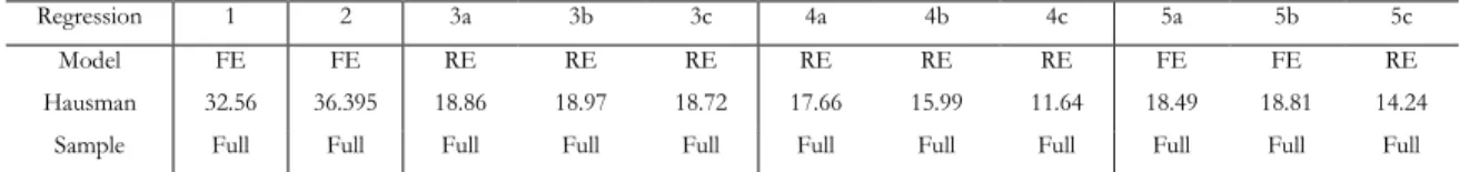
In this section, we present the results from the estimations of equations (4.12) and (4.13). We first estimated the model considering Panel I (UN Data) which includes all the 100 countries listed in the Appendix B. Countries are then divided by geographic groups, income levels and export clubs to analyse eventual diversities.

Table 4.1 – Panel data estimation of the relationship between economic structure and

wage growth (Main Results)

Regression 1 2 3a 3b 3c 4a 4b 4c 5a 5b 5c

Model FE FE RE RE RE RE RE RE FE FE RE

Hausman 32.56 36.395 18.86 18.97 18.72 17.66 15.99 11.64 18.49 18.81 14.24

Wage Out. Out. LC LC LC LC LC LC LC LC LC

RD Pat. Pat. Pat. Pat. Pat. Exp. Exp. Exp. Exp. Exp. Exp.

IQ Bud. Bud. Bud. Bud. Bud. Bud. Bud. Bud. FH FH FH

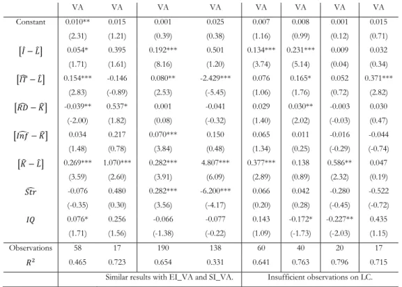
Str HHI VA HHI VAº HHI VA EI VA SI VA HHI VA EI VA SI VA HHI VA EI VA SI VA Constant 0.003 (1.34) 0.003 (0.19) 0.037 (0.60) 0.029 (0.46) 0.098 (1.47) 0.043 (1.40) 0.044 (1.38) 0.004 (0.13) 0.004 (0.69) 0.003 (0.53) 0.006* (1.86) [𝐼̂ − 𝐿̂] 0.149*** (9.71) 0.147*** (10.02) 0.429 (1.21) 0.634* (1.80) 1.116*** (3.52) 0.918** (2.15) 1.173*** (2.79) 1.550*** (4.02) 0.177*** (8.45) 0.176*** (8.38) 0.167*** (8.74) [𝐼𝑇̂ − 𝐿̂] 0.078*** (3.08) 0.078*** (3.05) -2.140*** (-5.62) -2.011*** (-5.12) -2.311*** (-5.93) -2.377*** (-4.82) -2.278*** (-4.47) -2.570*** (-5.20) 0.079** (2.42) 0.079** (2.37) 0.118*** (3.93) [𝑅𝐷̂ − 𝐾̂] 0.002 (0.26) 0.001 (0.23) -0.029 (-0.26) -0.038 (-0.33) 0.083 (0.71) -0.562* (-1.72) -0.527 (-1.58) -0.658** (-1.98) 0.016 (0.98) 0.018 (1.15) 0.024 (1.61) [𝐼𝑛𝑓̂ − 𝐾̂] 0.039*** (2.98) 0.038*** (2.95) 0.127 (0.51) 0.088 (0.35) 0.060 (0.24) 0.080 (0.26) 0.056 (0.18) 0.035 (0.11) 0.012 (0.70) 0.011 (0.67) 0.018 (1.25) [𝐾̂ − 𝐿̂] 0.240*** (4.81) 0.241*** (4.83) 4.167*** (6.22) 4.062*** (5.94) 4.155*** (6.07) 4.236*** (5.13) 4.158*** (4.93) 4.008*** (4.80) 0.167*** (2.68) 0.177*** (2.85) 0.190*** (3.59) 𝑆𝑡𝑟̂ 0.030 (0.41) 0.000 (0.00) -6.142*** (-4.61) 12.227*** (3.73) -2.463*** (-3.75) -6.347*** (-4.10) 13.050*** (3.37) -3.214*** (-3.80) 0.213** (2.60) -0.464** (-2.41) 0.150*** (3.48) 𝐼𝑄 -0.038 (-1.07) -0.039 (-1.07) -0.145 (-0.48) -0.197 (-0.64) -0.064 (-0.21) -0.129 (-0.33) -0.221 (-0.56) -0.037 (-0.10) 0.001 (0.17) 0.002 (0.27) -0.003 (-0.90) Observations 385 385 167 167 167 127 127 127 220 220 220 𝑅2 _{0.471 0.471 0.304 0.281 0.269 0.359 0.338 0.349 0.518 0.515 0.525}

Similar results with EI_VA and SI_VA.

Notes: The dependent variable is the wage growth rate, measured either by output per worker (Out.) or labour compensation (LC). Time dummy variables are not presented due to space limitations. The t-statistics are in parentheses. Level of significance: *** 1%; ** 5%; * 10%. Estimations obtained with Stata software. º On regression 2, economic structure (Str) is measured in absolute values, not in growth rates.

Source: Authors own calculations.

Table 4.1 presents the main results for the panel data estimation of the relationship between economic structure and economic growth. We perform the Hausman test22 _for

each regression in order to assess the most adequate estimation procedure – Random effects (RE) or Fixed Effects (FE). The majority of the regressions was estimated considering the random effects model, which assumes no correlation between country-specific effects with the other regressors.

In regressions 1 and 2, we use output per worker (Out.), total patent applications (Pat.), and general government net lending/borrowing in percentage of GDP (Bud.) as measures of wage (W), research and development (RD), and institutional quality (IQ), respectively. Economic structure (Str) is measured by applying the Herfindahl-Hirschman index (HHI) to 1-digit sectoral value-added (VA) data. However, while in regression 1 economic structure is measured by growth rates, in regression 2 it was measured in absolute values. The results show no difference when we run the model with economic