M
ASTER
Monetary and Financial Economics
M
ASTER
´
S
F
INAL
W
ORK
D
ISSERTATION
S
YSTEMIC
R
ISK
I
NDICATORS
–
T
HE
C
ASE OF
P
ORTUGAL
S
INA
F
AZLOLLAHZADEH
E
ILAGHI
M
ASTER
Monetary and Financial Economics
M
ASTER
´
S
F
INAL
W
ORK
D
ISSERTATION
S
YSTEMIC
R
ISK
I
NDICATORS
–
T
HE
C
ASE OF
P
ORTUGAL
S
INA
F
AZLOLLAHZADEH
E
ILAGHI
S
UPERVISION:
D
R.
J
ORGEB
ARROSL
UISi GLOSSARY
AR – Autoregression.
BIS – Bank for International Settlements. CCA – Contingent Claim Analysis. CDS – Credit Default Swap.
CISS – Composite Indicator of Systemic Stress. CoVaR – Conditional Value at Risk.
DIP – Distress Insurance Premium. ECB – European Central Bank. ES – Expected Shortfall. FI – Financial Institution.
FSB – Financial Stability Board. FSI –Financial Stability Index. IMF – International Monetary Fund.
LRMES – Long Run Marginal Expected Shortfall. MES – Marginal Expected Shortfall.
OLS – Ordinary Linear Regression.
Option-iPoD – Option-implied Probability of Default. PCA – Principal Component Analysis.
PD – Probability of Default.
RAMSI – Risk Assessment Model for Systemic Institutions. SES – Systemic Expected Shortfall.
SND – Standard Normal Distribution. SRISK – Systemic Risk Index.
ii TED – Treasury-EuroDollar rate.
iii
ABSTRACT,KEYWORDS AND JELCODES
This dissertation is an effort to shed more light upon systemic risk of Portuguese financial systems. At first, companies listed in Portuguese stock market index (PSI-20) is considered, and then, the attention is shifted to banking system. Considering the first part, the PSI-20 index is considered as financial system index, and spillover effect and marginal risk contribution of companies to the system is detected. CoVaR and ΔCoVaR are the risk indicators used for this purpose. CoVaR shows the spillover effect of a company or system being distressed to another, and ΔCoVaR measures the contribution of a firm or system to another one if its state changes from median to distressed situation. CoVaR for all firms were so close i.e. they have the same spillover effect, but ΔCoVaR were different i.e. their marginal risk contribution is different. Secondly, banking system of Portugal is considered separately, and the same indicators are used to quantify the linkage of banks and the system. It is concluded that Banco Comercial Português (BCP) is adding less risk to other banks and the system compared to the risk contributed to it. Thirdly, due to interconnectedness of banks all over the world, the spillover effect and risk contribution of major international banks on Portuguese banking system and vice versa are analysed to figure out which banks affect Portuguese financial system more in case of being distressed, and the other way around. Lastly, we estimated CoVaR and ΔCoVaR for Banco Espírito Santo (BES). Since BES was resolved in 2014, which was a systemic event, it sounded interesting to detect which international banks were more affected by the event, and which one contributed more risk to BES before its resolution. The conclusion was that the Portuguese banking system and BES is more linked to European banks that non-European banks.
KEYWORDS: Systemic Risk; Financial Institutions; Financial Crises; Risk Indicators;
Financial System
iv TABLE OF CONTENTS
Glossary ... i
Abstract, Keywords and JEL Codes ... iii
Table of Contents... iv
Table of Figures ... vi
Acknowledgments ... vii
1. Introduction ... 8
2. Systemic Risk Indicators ... 11
2.1. Volatility Indices ... 11
2.2. TED Spreads ... 12
2.3. Yield Curve Slope ... 12
2.4. Distress Insurance Premium (DIP) ... 13
2.5. CoVaR ... 14
2.6. Systemic Expected Shortfall ... 15
2.7. SRISK ... 16
2.8. Option-iPoD... 18
2.9. CoRisk ... 20
2.10. Principal Components Analysis and Granger-Causality ... 21
2.11. Composite Indicator of Systemic Stress (CISS) ... 22
2.12. Risk Assessment Model for Systemic Institutions (RAMSI) ... 23
2.13. Markov Regime Switching Autoregressive Conditional Heteroskedastic Model (SWARCH) ... 24
2.14. Conclusion on Reviewed Indicators ... 25
2.15. ΔCoVaR Estimation ... 26
v
3. Empirical study ... 28
3.1. Risk Contribution of Companies listed in PSI 20... 28
3.2. Portuguese banking system ... 31
3.3. Risk linkage between international banks and the Portuguese banking system ... 34
3.4. International banks and BES risk contribution ... 38
4. Conclusion ... 41
References ... 43
vi TABLE OF FIGURES
Figure 1– flow-chart of RAMSI model ... 24 Figure 2 – 5% VaR of PSI 20, EuroStoxx 50, and PSI 20 listed firms ... 29 Figure 3 – 5% VaR and 5% CoVaR of PSI 20, EuroStoxx 50, and PSI20 listed firms ... 30
Figure 4 – 5% VaR and 5% ΔCoVaR of PSI 20, EuroStoxx 50, and PSI20 listed firms ... 31
vii ACKNOWLEDGMENTS
First, I wish to express my gratitude to Professor Jorge Barros Luis for his continuous encouragement and guidance.
I am also grateful to my friends Ehsan Movahed and Mehrdad Mohammadi for their steady spiritual support from thousands of kilometres away.
Finally, many thanks go to my family for their patience, support, and sacrifice, not only during writing this thesis, but also at every single moment of my life.
8
SYSTEMIC RISK INDICATORS – THE CASE OF PORTUGAL By Sina F. Eilaghi
THIS dissertation provides new insights on systemic risk of Portuguese financial system using CoVaR and ΔCoVaR indicators, which are aimed to estimate spillover effects and risk contribution of an institution or a system to another institution or system. Both stock market and banking system of Portugal are analysed, and most systemically important companies and banks are determined. Also, risk interconnectedness of Portuguese banking system and a resolved bank, BES, with major international banks are quantified applying the same indicators.
1.INTRODUCTION
The global financial crisis of 2007 followed by the European Government debt crisis starting in 2010 revealed the inadequacies of microprudential, firm-level oversight, supervision approach in managing financial stability. Although diversification helps in managing idiosyncratic risk of an individual firm, it boosts risk propagation and increases systemic risk. After the recent crises, academics and regulators focused their attention on designing systemic risk indicators so as to predict and mitigate systemic risk ex-ante. Through Basel III and by the creation of macroprudential regulations, regulators tried to tackle the fragility of financial system. Indeed, Basel III provided provisions to limit overleveraging and augmented capital requirement for financial institutions. However, due to complex and ever-changing nature of financial environment, forecasting a possible systemic event is not straightforward. There have been quite a few efforts to detect systemic events ex-ante including systemic risk indicators, some of which are listed in the next chapter.
The first step to measure a variable is to define it. There are different definitions in the literature for systemic risk. Billio et al. (2010) defines systemic risk as “any set of circumstances that threatens the stability of or public confidence in financial system”. In response to a request from G-20 countries, the IMF, the FSB and the BIS provided systemic risk definition as “the risk that disruptions to financial services, triggered by impairments in the financial system, could affect the real economy” (Chan-Lau (2013)). In a simple word, systemic risk is the probability of a chain reaction in financial institutions after an individual institution defaulted. Indeed, systemic risk threatens the financial system as a whole in contrast to idiosyncratic risk which only considers the risk of loss at firm level. On the other side of the coin, each individual institution contributes
9
to systemic risk based on its liquidity risk, credit risk, leverage, and interconnectedness with other financial institutions. Contributing to systemic risk could be discouraged through taxation or penalties for firms that add more risk putting financial stability in jeopardy since systemic events, although not very common, endanger public welfare significantly.
Due to being systemically significant, the US and the Eurozone received a great amount of attention, and many efforts have been made to capture aggregate systemic risk in these countries, as well as detecting financial institutions with the largest contributions to systemic risk. However, less systemically important countries also need to be aware of their systemic risk situation, in order to be able to make better and timely decisions in the emergence of systemic events and prevent large loses. For example, they should know which industries or companies are more responsible for endangering their financial stability and implement actions to restrict their risk contribution ex-ante.
In this thesis, we focused on systemic risk of Portugal. First, we concentrated on the impact of Portuguese firms listed in PSI-20 index on the Portuguese financial stability. The purpose of this study is to identify the most systemically important companies and industries which add more risk to the financial system and quantify their contributions. The Value at Risk (VaR) methodology is used to measure the idiosyncratic risk of each firm independently from the financial system. Then, Adrian and Brunnermeier (2016) methodology of Conditional Value at Risk (CoVaR) and ∆CoVaR are applied. The CoVaR is an extension of VaR and indicates the value at risk of a financial system as a whole, conditional on having a financial institution being in distressed state. The ∆CoVaR is defined as the difference between the VaR of financial system conditional on having a financial institution being in distress and that of the same financial institution being in the median state. Intuitively, ∆CoVaR metrics quantifies the marginal contribution of each financial institution to systemic risk. Also, the Eurostoxx50 index, stock index of Eurozone stocks, is considered to measure the linkage between Eurozone and Portuguese stock markets. The question we tried to answer in this part is which Portuguese company among the PSI-20 added more risk to Portuguese financial system.
Secondly, three Portuguese banks listed in stock market for a long enough period of time were considered, and a banking system return variable was built. Then, the risk
10
linkage between Portuguese banks, and the risk linkage between each Portuguese bank with the built Portuguese banking system index is calculated using CoVaR and ∆CoVaR. The goal is to figure out which of the three banks is contributing more risk to other banks and the banking system.
Thirdly, we considered the interconnectedness of Portuguese banking system with major banks of the world. Since Portuguese banks are not working in isolation of other banks of the world, we tried to capture the risk contribution in both directions: from individual international banks to Portuguese banking system and vice versa. An international banking system index is built to represent the international banking system and we used it to detect risk interconnectedness of Portugal and the world as a whole.
Lastly, since Banco Espírito Santo (BES), the then largest Portuguese privately owned bank, was resolved in 2014, which can be considered as a systemic event, we studied the risk linkage of the international banks and BES to detect which banks were more affected by BES, and which one was contributing more risk to it. In this section, we again calculated CoVaR and ∆CoVaR indicators.
The structure of this thesis is organised as follows; In the second chapter, the main systemic risk indicators suggested in the literature are explained briefly. There is a wide range of indicators from simple ones like volatility indices to more complex methodologies developed recently. Methodologies used in the analysis of Portugal’s systemic risk in this study -including VaR, CoVaR, and ∆CoVaR- are explained with more details. In the third chapter, the result of the four studies mentioned above are discussed in detail. Finally, in the last chapter, a brief conclusion is presented.
11
2.SYSTEMIC RISK INDICATORS
Systemic risk is a multifaceted issue, which can be triggered from various directions. Therefore, different metrics and indicators are required to track the build-up of aggregate risk in financial system. The creation of early-warning signals helps financial institutes and regulators to manage a potential systemic event better by being forearmed. For that reason, a diversity of metrics and models are built to capture systemic risk by considering different aspects of the concept. In this chapter, the most common systemic risk indicators including those applied in the empirical study of next chapter are reviewed. In addition to the main papers, Di Cesare and Picco (2018) and Bisias et al. (2012) are two review papers that are used in this section.
2.1. Volatility Indices
Economic agents manage their risk behaviour based on their risk perception. However, risk perception may differ from real risk. Minsky’s (1977) instability theory claims that low risk perception induces firms to take higher risks, which results in the building-up of aggregate risk and finally leads to financial crisis. In summary, stability can be destabilizing.
Danielsson and Valenzuela (2016) expressed two channels through which volatility may signal a pending financial panic: low volatility channel and high volatility channel. When volatility is low, firms realize it is lower than expectations, which makes them more optimistic and induce them to be more risk-taker. At this time, banks accept less creditworthy borrowers, leading to build-up of systemic risk and more defaults in the future.
On the other hand, high volatility raises uncertainty about future cash flow and economic growth, i.e. the fear of future increases. Some economic agents may avoid that fear by selling some of their investments and opting for less risky ones, which may lead to price reduction and even fire sale. Therefore, high volatility signals pending crisis. This chain of events is called high volatility channel. However, sometimes high volatility is a result of crisis when the crisis happens surprisingly like the 2010 Flash Crash, in which the withdrawal of orders extremely amplified decrease of the Dow Jones Industrial Average, more than 1000 points in only 10 minutes.
12
Danielsson and Valenzuela (2016) found that prolonged periods of relatively low volatility have predictive power, not the level of volatility. The level of volatility differs from country to country and along time. They defined “volatility gap”, which measures volatility deviation from its trend, to gauge relatively low or high volatility. Also, they found that low volatility results in credit build-up, which adds more risk to the financial system and imperils financial stability.
All in all, being included in macro-prudential monitoring frameworks, volatility of financial markets is one of the most common indicators used in policymaking decisions. The low volatility channel is more significant farther from the beginning of crises, but the high channel is more crucial closer to when crisis is about to start.
2.2. TED Spreads
The TED spread is computed as the spread between three-month LIBOR, at which banks are able to borrow money from each other, and interest rate of three-month Treasury Bills, at which government can borrow for a three month horizon. Thus, this spread works as a barometer for banking system stability (Boudt et al. (2017)). Increase in TED spread indicates either less creditworthiness assessment of banks by other banks, so they ask more interest from other banks to compensate the higher risk of default or financiers are increasing their investment in T-bills due to lower ratio of stock market return to risk. Conversely, a decrease in this spread suggests that banks attached lower probability of default to other banks, making them more willing to lend and therefore less interest is asked or investors prefer to invest in stock market rather than T-Bills. Acharya and Skeie (2011) suggested that the TED spread is able to capture liquidity risk, counterparty risk, flight-to-quality, and flight-to-liquidity.
In empirical studies, peaks of the spread are followed by systemic events (Wu and Hong (2012)).
2.3. Yield Curve Slope
The yield curve, being the graphical representation of the term structure of interest rates, illustrates the relationship between interest rates and maturities for risk-free bonds
13
(Martellini, 2003, p. 63). The yield curve slope, calculated as the difference between the long-term and the short-term yield, helps in forecasting changes in short-term interest rate and macroeconomics conditions. If the slope of the curve is positive, the longer maturity bond’s yield is higher than shorter maturity one, which is usually called a normal yield curve, interpreted as illustrating prospects of economic growth, and therefore less systemic risk in the financial system. During transitions from economic growth to recession periods, long-term and short-term yields become very close, i.e. the yield curve is close to flat. When the yield curve slope is negative, i.e. short-term yields are greater than long-term yields, it is a sign of upcoming recession. Therefore, the more negative the yield curve slope, the higher the systemic risk in the financial system.
2.4. Distress Insurance Premium (DIP)
Huang et al. (2011) introduced a new forward-looking systemic risk indicator called “Distress Insurance Premium (DIP)”, which is the theoretical insurance premium to protect against systemic failure with significant losses in the banking system. Indeed, DIP measures the expected loss equal or higher than a threshold of the total liabilities of banks. It is calculated based on the price of credit default swap (CDS) spreads and price of banks’ shares in stock exchange market, both of which are available in real-time daily timeframe i.e. DIP may be updated on a daily basis. The DIP computing requires the calculation of the probability of default (PD) of each financial institution and asset return correlations. The first component, PDs, is calculated using CDS spreads, while the second component, asset return correlations, is calculated based on equity return correlations.
This indicator increases with both the PDs and asset return correlations. The higher the CDS spreads, the higher the PDs, the greater the systemic risk in the financial system. Similarly, higher correlation in asset returns represents a higher exposure to common risk components, which means higher systemic risk in financial system and will also corresponds to higher value of DIP.
Huang et al. (2012) augmented their first version of the DIP indicator by three improvements. First, they used a dynamic conditional correlation model instead of a time invariant model to estimate asset return correlations. The second improvement was regarding PDs calculation, using expected default frequency from Moody’s KMV,
14
instead of CDS spreads. The difference is that, while CDS spreads gives risk-neutral PDs, Moody’s KMV provides a measure of actual PDs. Lastly, this analysis measures the marginal contribution of individual banks to the whole systemic risk in addition to calculating aggregate systemic risk indicator.
2.5. CoVaR
According to Adrian and Brunnermeier (2016), Conditional Value at Risk (CoVaR) is an indicator of systemic risk which is built on the Value at Risk (VaR) concept. The VaR is the highest amount of estimated losses under a given distribution, considering a given degree of confidence and a given period of time (Jorion 2006). The VaR of an institution at q percentile is mathematically defined as:
(1) Pr(𝑋 ≤ 𝑉𝑎𝑅𝑞) = 𝑞
where X is the return value of institution. Equation (1) means that the probability of having asset returns not higher than VaR for the following period of time is equal to q, while the probability of having asset returns higher than the VaR value is at least 1-q.
The CoVaR of an institution refers to the value at risk of the financial system as a whole, conditional on a particular state of the institution. Since during distressed periods the financial institution’s equity return shows significant co-movement in comparison with stable periods, the VaR, which only takes into consideration idiosyncratic risk, cannot accurately mirror systemic risk. The idea of CoVaR is to capture change in the value at risk stemming from the distressed financial institutions due to the fact that those distressed firms change the distribution of asset values. Indeed, CoVaR helps in understanding spillover effects. The 𝐶𝑜𝑉𝑎𝑅𝑞𝑗|𝑖 is then the value at risk of j, which can be either the whole system or an institution, conditional on the event that institution i reaches its VaR value. It is mathematically represented as follows:
(2) Pr(𝑋𝑗 ≤ 𝐶𝑜𝑉𝑎𝑅 𝑞 𝑗|𝑖
| 𝑋𝑖 = 𝑉𝑎𝑅
𝑞𝑖) = 𝑞
where q is the quantile and X denotes asset returns of an institution or the financial system.
15
The marginal contribution of an individual institution i to another institution j (j can be the whole systemic risk) is calculated as the difference between 𝐶𝑜𝑉𝑎𝑅𝑞𝑗|𝑖, which is the VaR of institution j when institution i is in distress, and 𝐶𝑜𝑉𝑎𝑅50%𝑗|𝑖 , which denotes the VaR of return of institution j when institution i is performing at its normal state (median or q = 50%). The mathematic formula is as follows:
(3) Δ𝐶𝑜𝑉𝑎𝑅𝑞𝑗|𝑖= 𝐶𝑜𝑉𝑎𝑅𝑞𝑗|𝑋𝑖=𝑉𝑎𝑅𝑞
𝑖
− 𝐶𝑜𝑉𝑎𝑅𝑞𝑗|𝑋𝑖=𝑉𝑎𝑅50%𝑖
Δ𝐶𝑜𝑉𝑎𝑅 measures how much each individual institution adds to the aggregate systemic risk. In other words, Δ𝐶𝑜𝑉𝑎𝑅 measures the comovement of overall systemic risk with a particular distressed institution.
Δ𝐶𝑜𝑉𝑎𝑅 provides several advantages in comparison to previously mentioned indicators. First of all, as mentioned before, it calculates the risk contribution of each firm, indicating the degree to which each institution is responsible for a systemic event. Secondly, Δ𝐶𝑜𝑉𝑎𝑅 can gauge the spillover effects between different institutions, since Δ𝐶𝑜𝑉𝑎𝑅𝑗|𝑖 measures the increased risk of institution j accompanied by distress in
institution i. Thirdly, Δ𝐶𝑜𝑉𝑎𝑅 can be extended for other risk indicators such as “expected shortfall” (ES) which will be discussed later. Lastly, it is also able to gauge the risk that systemic events can add to individual institution’s risk, which is the reverse direction of spillover discussed before.
2.6. Systemic Expected Shortfall
Like VaR, Expected Shortfall (ES) is a risk measure at individual institution level which is defined as the potential value that a firm might lose when a systemic event occurs (Acharya et al. (2010)). Mathematical representation of ES is as follows:
(4) 𝐸𝑆𝛼= −𝐸[𝑅|𝑅 ≤ −𝑉𝑎𝑅𝛼]
where R is the asset return. So, ES is the expected loss on days with asset loss higher than its VaR.
Considering the whole banking system instead of a bank, banks in banking system play the same role as groups or trading desks in an individual bank. Financial institutions
16
required to consider each group’s loss contribution to manage risk and capital allocation. Therefore, taking into account each group’s return, equation 4 can be rewritten as follows:
(5) 𝐸𝑆𝛼= − ∑ 𝑦𝑖 𝑖𝐸[𝑟𝑖|𝑅 ≤ −𝑉𝑎𝑅𝛼]
in which ri is the return of group i, yi is the group i’s weight in portfolio, and total
return, R, is equal to the weighed sum of group’s return (𝑅 = ∑ 𝑦𝑖 𝑖𝑟𝑖).
To obtain the sensitivity of total risk to the weight of trading desk i, called Marginal Expected Shortfall (MES), the derivative of ESα with respect to yi is calculated:
(6) 𝑀𝐸𝑆𝛼𝑖 = 𝜕𝐸𝑆𝛼
𝜕𝑦𝑖 = −𝐸[𝑟𝑖|𝑅 ≤ −𝑉𝑎𝑅𝛼]
The MESi measures the effect of group i’s risk appetite on the total risk taken by the
bank. As it can be seen in equation 6, MESi is the amount of group i’s loss conditional on
bank’s loss exceeded its VaR value.
The above-mentioned risk measure is used for analysing risk of the whole financial system. In this framework, R is the total banking system return, and MES measures bank
i’s losses conditional on poor performance of the banking system, i.e. when banking
system losses are higher than its VaR.
Acharya et al. (2010) then proposed the Systemic Expected Shortfall (SESi) measure which captures the expected contribution of bank i to systemic risk and defined it as follows:
(7) 𝑆𝐸𝑆𝑖 = −𝐸[𝑧𝑎𝑖− 𝑤𝑖| 𝑊 < 𝑧𝐴]
where wi is the bank i equity, z is a fraction, W is the total banking capital, and A is aggregate banking system asset. In other words, SES is the deviation of bank i’s equity from its expected value, which is a fraction of its asset, when W, aggregate capital of banking sector fell below z multiplied by total assets i.e. a systemic event occurred.
2.7. SRISK
Based on SES, Brownlees and Engle (2017) presented SRISK, which measures individual financial institutions contribution to systemic risk, and aggregate SRISK, which signals systemic event ex-ante by tracking undercapitalization possibility. The
17
authors defined SRISK as the expected capital shortfall of a firm conditional on a prolonged and severe downward trend in the market. It is a function of size, leverage and the long run MES (LRMES) of the financial institute. Similar to SES, SRISK is calculated using MES and in addition to LVG of the firm. However, there are differences in MES estimation. The SES solely applies financial market data to estimate MES, but the SRISK estimates MES using advanced econometrics model, which considers both market and balance sheet data.
The first step to compute SRISK is to mathematically define capital shortfall. Capital shortfall is computed as the difference between capital reserves hold by the financial institute and its equity as represented below:
(8) 𝐶𝑆𝑡 = 𝑘𝐴𝑡− 𝑊𝑡 = 𝑘(𝐷𝑡+ 𝑊𝑡) − 𝑊𝑡
where Wt is equity value in the market at time t, At is quasi assets value at time t, Dt
is the debt value (book value) at t, and k is the fraction of prudential capital. Considering Basel III regulatory framework, k can be thought as the Tier I capital ratio, which depends on risk-weighted assets (Wewel (2014)). In this methodology, a systemic event happens if the market return decline in absolute value is higher than a threshold, C, during a constant time interval, h.
(9) 𝑆𝑅𝐼𝑆𝐾𝑖,𝑡 = 𝐸𝑡[𝐶𝑆𝑖,𝑡+ℎ|𝑅𝑚,𝑡+1:𝑡+ℎ < 𝐶] = 𝑘𝐸𝑡[𝐷𝑖,𝑡+ℎ|𝑅𝑚,𝑡+1:𝑡+ℎ < 𝐶] −
(1 − 𝑘)𝐸𝑡[𝑊𝑖,𝑡+ℎ|𝑅𝑚,𝑡+1:𝑡+ℎ < 𝐶]
where Rm,t+1:t+h is the market return from t + 1 to t + h. the condition {𝑅𝑚,𝑡+1:𝑡+ℎ <
𝐶} demonstrate the occurrence of systemic event. The SRISK indicates the expected capital shortfall if the systemic event occurs. Assuming debts are not renegotiable ex-post, equation 9 is rewritten below:
(10) 𝑆𝑅𝐼𝑆𝐾𝑖,𝑡 = 𝑊𝑖,𝑡[𝑘𝐿𝑉𝐺𝑖,𝑡+ (1 − 𝑘)𝐿𝑅𝑀𝐸𝑆𝑖,𝑡− 1)
where 𝐿𝑅𝑀𝐸𝑆𝑖,𝑡 = −𝐸𝑡[𝑅𝑖,𝑡+1:𝑡+ℎ|𝑅𝑚,𝑡+1:𝑡+ℎ < 𝐶] and 𝐿𝑉𝐺𝑖,𝑡 = 𝐷𝑖,𝑡+𝑊𝑖,𝑡
𝑊𝑖,𝑡 , is
quasi-leverage ratio. Equation (10) indicates the dependence of SRISK to three components: a firm’s degree of leverage, its size, and expected equity price decline in the case of having a market decline.
18
A higher value of SRISK for an institution indicates higher expected capital shortfall in case of extreme distress in financial system, which means the institution is contributing more to systemic risk.
Based on SRISKi,t, aggregate SRISKt is introduced as an early warning systemic risk
indicator. Since during the crisis the surplus capital of banks with negative SRISK might not be available to help distressed institutions, only positive values of SRISK are summed up to calculate aggregate SRISK:
(11) 𝑆𝑅𝐼𝑆𝐾𝑡= ∑𝑁𝑖=1max(𝑆𝑅𝐼𝑆𝐾𝑖,𝑡, 0)
SRISKt tracks the build-up of expected capital shortfall and measures the capital
needed to be financed by the Government to bail out the whole system in the case of systemic events.
2.8. Option-iPoD
Based on Merton’s pricing model, Capuano (2008) introduced the Option-implied probability of default (Option-iPoD) framework to obtain the probability of default of a firm from equity option price. Since the principle of minimum cross-entropy is applied, the probability distribution is recoverable, and therefore, there is no need for distributional assumption. Another advantage of Option-iPoD is allowing for the endogenous estimation of the default barrier, a threshold level. The definition of probability of default is the probability that the firm’s asset value will become less than the default barrier.
The author mathematically defined probability of default as follows: (12) 𝑃𝑜𝐷(𝑋) = ∫ 𝑓𝑣(𝑉)𝑑𝑣
𝑋 0
where X represents the default barrier, fv is the probability density function, and V is
asset value.
The payoff of a call option written on the market value assets is the maximum between the equity price at maturity day and zero. According to Merton’s approach, the stock price can be considered as the price of a call option on the assets of the institution, while the strike price is the face value of on-balance sheet liabilities, i.e. the equity price is the
19
maximum between the firm’s asset value minus its liabilities and zero. Hence, an option written on another option is equivalent to an option written on a stock.
(13) 𝐶𝑇𝐾 = max(𝐸𝑇− 𝐾, 0) = max(𝑚𝑎𝑥(𝑉𝑇− 𝐷, 0) − 𝐾, 0) = max(𝑉𝑇− 𝐷 − 𝐾, 0)
where 𝐶𝑇𝐾 is the payoff of option at expiry date (T), ET is the equity price at T, K is
exercise price, VT is firm’s asset value at expiration, and D represents firm’s debt.
Two parameters are needed to be computed so as to calculate option-iPoD: the value of D, the default threshold related to the debt value, and VT , to calculate the probability
of having VT smaller than D. Capuano applied the cross-entropy to calculate the PD
implied by the prices of options. The objective function needed to be optimized is highly nonlinear, and therefore numerical methods are used. The objective function is presented below: (14) min 𝐷 { min𝑓(𝑉𝑇)∫ 𝑓(𝑉𝑇) log [ 𝑓(𝑉𝑇) 𝑓0(𝑉𝑇)] 𝑑𝑉𝑇 ∞ 𝑉𝑇=0 }
where 𝑓(𝑉𝑇) is the posterior density function of asset value and 𝑓0(𝑉
𝑇) is the
prior-knowledge of researcher on 𝑓(𝑉𝑇). 𝑓(𝑉𝑇) log [𝑓(𝑉𝑇)
𝑓0(𝑉𝑇)] represents the cross-entropy
between prior and posterior density functions (𝑓(𝑉𝑇) and 𝑓0(𝑉𝑇)). The first constrain of
the optimization problem is the equity value should correspond to the call option value written on the assets value i.e.:
(15) 𝐸0 = 𝑒−𝑟𝑇∫ max(𝑉 𝑇− 𝐷, 0) 𝑓(𝑉𝑇)𝑑𝑉𝑇 ∞ 𝑉𝑇=0 = 𝑒−𝑟𝑇∫ (𝑉 𝑇− 𝐷, 0)𝑓(𝑉𝑇)𝑑𝑉𝑇 ∞ 𝑉𝑇=𝐷
where 𝐸0 is today’s stock price.
The second constrain is the ability of posterior density to price observable option prices: (16) 𝐶0𝑖 = 𝑒−𝑟𝑇∫ max(𝑉𝑇− 𝐷 − 𝐾𝑖, 0) 𝑓(𝑉𝑇)𝑑𝑉𝑇 ∞ 𝑉𝑇=0 = 𝑒−𝑟𝑇∫𝑉∞ (𝑉𝑇− 𝐷 − 𝐾𝑖, 0)𝑓(𝑉𝑇)𝑑𝑉𝑇 𝑇=𝐷+𝐾𝑖
where 𝐶0𝑖 is the today price of call-option and i is the number of option contract. The last constrain is normalization constraint:
20 (17) ∫ 𝑓(𝑉𝑇)𝑑𝑉𝑇
∞
𝑉𝑇=0 = 1
Higher value of option-iPoD corresponds to higher risk of default of the institution, which can act as an early warning for the market. Its predictive power is shown in Capuano (2008) for the case of Bear Stearns failure in 14 March 2008, as option_iPoD started to provide warning signals on February 21.
2.9. CoRisk
Suggested by the IMF (2009a), CoRisk is an indicator that gauges the risk co-dependence of financial institutions. This indicator measures the percentage change in PD of an institution conditional on the risk of another institution and other risk drivers such as volatility indices or TED spread and its unconditional PD.
Since OLS regression fails to capture nonlinear relationships, quantile regression is applied for CoRisk calculation. In the Global Financial Stability Review of IMF (2009a), CoRisk is computed based on CDS of different firms. First, CDS estimate of institution i is obtained from a set of explanatory variables, including CDS prices of other institutions through the below-mentioned quantile regression formula:
(18) 𝐶𝐷𝑆𝑖,𝑡 = 𝛼𝑞𝑖 + ∑𝐾𝑘=1𝛽𝑞,𝑘𝑖 𝑅𝑘,𝑡+ 𝛽𝑞,𝑗𝑖 𝐶𝐷𝑆𝑗,𝑡+ 𝜖𝑖,𝑡
where CDSi,t is the credit default swap spread of firm i at day t, K is the number of
risk drivers, Rk,t is the risk factor value at day t, and q is the quantile parameter. 𝛽𝑞,𝑗𝑖 is the
regression coefficient, which provides intuition about the way CDS of institution j affects CDS of firm i. The optimization problem of equation (15) has to be solved in order to find quantiles for independent variables:
(19) min
𝛼𝑞𝑖𝛽𝑞,𝑘𝑖 𝛽𝑞,𝑗𝑖
∑ 𝜌𝑡 𝑞(𝐶𝐷𝑆𝑖,𝑡− 𝛼𝑞𝑖 − ∑𝑘=1𝐾 𝛽𝑞,𝑘𝑖 𝑅𝑘,𝑡 − 𝛽𝑞,𝑗𝑖 𝐶𝐷𝑆𝑗,𝑡) where ρq is defined as follows:
(20) 𝜌𝑞(𝑡) = {
𝑞 𝑓𝑜𝑟 𝜀𝑡≥ 0 (1 − 𝑞) 𝑓𝑜𝑟 𝜀𝑡< 0
Thus, the q, the quantile, takes a value between 0 and 1. Once the coefficients of quantile regression are obtained, the CoRisk indicator can be calculated as:
21 (21) 𝐶𝑜𝑅𝑖𝑠𝑘𝑖,𝑗𝑡 = 100 ∗ (𝛼𝑞 𝑖+∑ 𝛽 𝑞,𝑘𝑖 𝐾 𝑘=1 𝑅𝑘,𝑡+𝛽𝑞,𝑗𝑖 𝐶𝐷𝑆𝑗(𝑞) 𝐶𝐷𝑆𝑖(𝑞) − 1)
Usually a high value is considered for q such as 0.95. CDS(q) is the CDS spreads of the firm to the qth percentile of its historical values. The higher the CoRisk, the higher the probability of default of the institution i will be if institution j defaults. For example, if the CoRiskA,B with q equal to 0.95 is equal to 300 per cent, it means the risk of institution
A conditional on the risk of institution B is three hundred per cent higher than the risk related to 95th percentile of empirical distribution of institution A i.e. institution A is highly affected if institution B is distressed.
2.10. Principal Components Analysis and Granger-Causality
Billio et al. (2012) applied principal component analysis (PCA) and Granger-causality tests to introduce two measures that captures unconditional correlation, and then used it to assess to what extent the financial system sectors are linked.
The first indicator is based on PCA and aimed to detect changes in correlations between asset returns of different financial entities. PCA is a method that decomposes a set of correlated variables, which is volatility of equity return of FIs in their work, into a set of uncorrelated variables through orthogonal transformation. The obtained set of variables is called “principal components”, which has a smaller number of variables compared to the original one. However, it can illustrate original variables’ variance with high level of accuracy.
The higher the interconnectedness of FIs, the lower the number of synthetic components necessary to explain equity volatility. Therefore, PCA can be used to gauge connectedness among FIs.
The second method was Granger-causality test (linear and nonlinear), which is aimed to explore the direction of causality relationship between FIs and its statistically significance. This method reveals if past values in time series A contain more information that helps in predicting current changes in the values of time series B than the information gained using values of time series B alone, which means A Granger causes B. Therefore, Granger causality concept can help to check if an individual bank can Granger cause the financial system. Billio et. al. (2012) found that stock return of banks and insurance
22
companies influence that of hedge funds and brokers/dealers more than the other way around. Billio et. al. (2013) extended previous research by considering fair-value of credit default swap spreads instead of returns on equities using contingent claim analysis (CCA). Also, connection of sovereigns with each other and sovereigns with FIs is analysed.
The two abovementioned measures complement CoVaR, SES, and DIP, through the estimation of connectedness between returns of FIs.
2.11. Composite Indicator of Systemic Stress (CISS)
Suggested in ECB (2011), the CISS is a composite financial stability index (FSI) aimed to gauge the state of instability (Hollo et al. (2012)). As it is understandable from its name, CISS combines individual risk indicators into a new indicator. It is also able to capture systemic risk arising from the effect of the real economy on financial system and vice-versa. Another novelty brought by CISS is the utilisation of portfolio theory in order to aggregate sub-indices into a single statistic.
The CISS concentrates on systemic dimension of stress by considering 15 measures of financial instability and putting them into 5 categories: the foreign exchange market, the equity market, the financial intermediaries sector, the money market, and the bond market. Then, an instability sub-index is calculated for each of them. Finally, computed sub-indices will be transformed into CISS using the portfolio theory rules, which applies time-varying cross-correlations to calculate weights of sub-indices. Events with more predominant negative effect, and therefore higher systemic effect on different markets simultaneously have relatively higher weights.
Hollo et al. (2012) illustrate the ability of the CISS in warning systemic events
ex-ante, with peaks in the indicator being associated with distress in the financial system.
The application of the CISS to euro-zone data also shows that the CISS is robust to the arrival of new data, which helps in avoiding reclassification of events. Another merit of CISS is that the indicator can be computed in real-time, since the needed data is mostly market-based. However, the CISS cannot detect the origins of distress and the channels through which instability can be transmitted.
23
All in all, higher CISS represents higher instability, uncertainty, information asymmetry, and lower tendency to keep illiquid and risky assets, which, in turn, leads to higher systemic risk in the financial system.
2.12. Risk Assessment Model for Systemic Institutions (RAMSI)
Introduced by the Bank of England, RAMSI is a large-scale model of main UK banks, which is designed with the purpose of assessing financial stability of UK banking sector through capturing liquidity and solvency risk of banks (Aikman et al. 2011). RAMSI is created in a way to be more focused on overall systemic risk rather than an individual bank’s risk. Alessandri et. al. (2009) describes the RAMSI structure and the way a macroeconomic shock propagates to financial system and its feedback effect, which can be seen in Figure 1.
Considering business and credit cycle durations, the model is run over 12 quarters, which is the same duration as the one central banks usually consider for stress testing financial systems. Macroeconomic risk factors for US and UK are estimated for each quarter, which are used to compute yield curves and PDs. Then, considering different risk factors together, the effects of the three first-round on the ten largest UK banks is assessed. Firstly, returns on banks’ assets are modelled and the balance sheet will be updated accordingly with the assumptions that profitable banks keep their initial tier 1 capital and leverage ratios, and loss making banks have a minimum threshold for tier 1 capital to be considered as defaulted. Having no defaulted bank means the simulation is over. Secondly, credit loss is taken into consideration when the loss of a bankrupt bank is propagated to other banks through counterparty credit losses or mark-to-market losses, and balance sheets will be rebalanced. Banks that survived in the first-round might default in this stage, which oblige us to consider its feedback effect. Lastly, the influence of net interest income is calculated.
24
Figure 1– flow-chart of RAMSI model
Required data for running the RAMSI includes income statement of banks, balance sheet of banks, and forecast of macro financial variables. Also, for simplicity, some behavioural assumptions are considered on the way banks react to macroeconomic shocks; however, it has a drawback that banks are not optimizing their situations. The output of RAMSI is the profit of banks before tax, which is the sum of net interest income, trading income, operating expenses (with negative sign), credit losses (with negative sign) and other income.
2.13. Markov Regime Switching Autoregressive Conditional Heteroskedastic Model (SWARCH)
Gonzalez-Hermosillo et. al. (2009) opted for a SWARCH model by Hamilton and Susmel (1994) to determine whether the risk state of financial system is low, medium, or high and the probability of having a financial distress. SWARCH is an ARCH model with state-dependent parameters. Indeed, the SWARCH model uses the dynamics of market risk condition indicators, including the VIX, the EUR-USD forex swap, and the TED
25
spread to distinguish the volatility state. The likelihood of change of volatility state between low, medium, and high is modelled through a Markov chain, which is as follows: (22) 𝑃(𝑠𝑡 = 𝑗|𝑠𝑡−1= 𝑖, 𝑠𝑡−1= 𝑘, … , 𝑦𝑡−1, 𝑦𝑡−2) = 𝑃(𝑠𝑡 = 𝑗|𝑠𝑡−1= 𝑖) =
= 𝑝𝑖𝑗
where yt denoting observed variables vector, st denoting an unobserved random
variable, and pij is the probability of changing state of financial system from i to j.
Gonzalez-Hermosillo et. al. (2009) used the following AR (1) process: (23) 𝑦𝑡 = 𝛼 + ∅𝑦𝑡−1+ 𝜀𝑡
in which 𝜀𝑡 is an error term with the following characteristics:
(24) {
ℎ𝑡2 = 𝑎0+ ∑𝑞𝑖=1𝑎𝑖𝜀̃𝑡−𝑖2 + 𝛿𝑑𝑡−1𝜀̃𝑡−12
𝜀̃𝑡= ℎ𝑡𝜗𝑡
𝜀𝑡 = √𝑔𝑆𝑡𝜀̃ 𝑡 where:
• ℎ𝑡2 is the time-varying variance
• 𝜗𝑡 has a standard normal distribution (SND) • 𝑆𝑡 ∈ {1,2,3} is the set of states
• 𝑑𝑡−1 is equal to 0 for 𝜀̃𝑡 > 0, and 1 otherwise
• 𝑔𝑆𝑡 is scaling factor, which is normalized to 1 when volatility regime is low So as to make sure about stationarity, first-difference variables are used.
The advantage of this model is that it accepts state-dependent parameters, and its disadvantage is its need for high-frequent data due to being univariate.
2.14. Conclusion on Reviewed Indicators
Several systemic indicators have been developed to signal policy makers and banks about impending systemic events. Some of the most useful and well-known indicators were briefly reviewed in this chapter, having most of them been developed after the great recession started in 2007, i.e. after that the need for macroprudential regulation become more heavily felt.
26
Before starting the analysis, Δ𝐶𝑜𝑉𝑎𝑅 estimation and calculation of market value of total assets return of FIs need to be explained in the following subsections.
2.15. ΔCoVaR Estimation
One of the practical methods to estimate CoVaR and Δ𝐶𝑜𝑉𝑎𝑅 is applying quantile regression. Quantile regression is similar to ordinary linear regression (OLS) with the possibility to consider the relation of regressors and a specific quantile of regressand. Quantile regression can give us insights about the conditional distribution when important information lies in the tails of distribution. Coefficients of a quantile regression predict the change in a particular quantile of regressand if the related regressor changes in one unit. Since in CoVaR and Δ𝐶𝑜𝑉𝑎𝑅 calculation, the major concern is the change in 5% quantile, the quantile regression is proper.
The quantile regression estimation is described as follows: (25) 𝑋̂𝑞𝑗|𝑋𝑖 = 𝛼̂𝑞𝑖 + 𝛽̂
𝑞𝑖𝑋𝑖
where 𝑋̂𝑞𝑗|𝑋𝑖 is the estimated value for the related quantile of institution j (or financial system) conditional on the realized return of institution i, which means that:
(26) 𝐶𝑜𝑉𝑎𝑅𝑞𝑗|𝑋𝑖 = 𝑋̂𝑞𝑗|𝑋𝑖
i.e. the estimated value of the quantile q of institution (system) j return conditional on Xi is the VaR of institution j conditional on Xi. Considering prediction for 𝑉𝑎𝑅
𝑞𝑖,
CoVaR can be computed by: (27) 𝐶𝑜𝑉𝑎𝑅̂ 𝑞𝑗|𝑋𝑖=𝑉𝑎𝑅𝑞
𝑖
= 𝑉𝑎𝑅̂𝑞𝑗 | 𝑉𝑎𝑅𝑞𝑖 = 𝛼̂𝑞𝑖 + 𝛽̂𝑞𝑖𝑉𝑎𝑅𝑞𝑖
Therefore, by calculating 𝑉𝑎𝑅𝑞𝑖 from related quantile of firm i’s returns itself, and
finally, Δ𝐶𝑜𝑉𝑎𝑅 can be estimated as follows: (28) 𝛥𝐶𝑜𝑉𝑎𝑅̂ 𝑞𝑗|𝑖 = 𝛽̂𝑞𝑖(𝑉𝑎𝑅𝑞𝑖 − 𝑉𝑎𝑅50𝑖 )
27
2.16. Calculation of Market Value of Total Assets Return of FIs
in order to calculate the return of a FI the methodology developed by Adrian and Brunnermeier is applied here, in which it is assumed that the returns of the market value of total assets of each bank is highly linked to the credit granted to debtors. Therefore, the return, is calculated as follows:
(29) 𝑋𝑡𝑖 = 𝑀𝐸𝑑𝑖 (𝐵𝐴𝑑 𝑖 𝐵𝐸𝑑𝑖)−𝑀𝐸𝑑−1 𝑖 (𝐵𝐴𝑑−1𝑖 𝐵𝐸𝑑−1𝑖 ) 𝑀𝐸𝑑−1𝑖 (𝐵𝐴𝑑−1 𝑖 𝐵𝐸𝑑−1𝑖 ) = 𝑀𝐴𝑑𝑖 −𝑀𝐴𝑑−1𝑖 𝑀𝐴𝑑−1𝑖
in which 𝑀𝐸𝑑𝑖 is the market value of total equity of firm i at day d, 𝐵𝐴𝑑𝑖 is the book value of total assets firm i at day d, 𝐵𝐸𝑑𝑖 is the book value of total equity of firm i at day
d, and 𝑀𝐴𝑑𝑖 is the market value total asset of firm i at day d. 𝑀𝐸𝑑
𝑖 𝐵𝐸𝑑𝑖
is the price-to-book value of equity which is available on Bloomberg. Also, 𝐵𝐴𝑑𝑖 is achieved through Bloomberg terminal, and the daily returns of market value of total assets are calculated.
28 3.EMPIRICAL STUDY
In this section, we conducted four empirical studies regarding systemic risk in the Portuguese financial system. In the first one, we considered the companies used to build PSI20 index and the index itself, which is considered as the representative index of the Portuguese Stock Exchange (Euronext Lisbon), in order to analyse the risk contribution of each company to the financial system. In this study, VaR, CoVaR, and Δ𝐶𝑜𝑉𝑎𝑅 are calculated for each company.
The second study is regarding the Portuguese banking system and the interconnectedness of banks and the Portuguese banking system is calculated. Since the Portuguese banking system is linked to international banks, in the third study, 47 international banks are selected and CoVaR and Δ𝐶𝑜𝑉𝑎𝑅 are estimated to indicate risk contribution of international banks to the Portuguese banking system and vice versa. Finally, we focused on the resolution of Banco Espírito Santo (BES). The idea is to estimate the risk contribution of BES to the Portuguese banking system, international banking system and each international bank considered before the resolution, and vice versa.
3.1. Risk Contribution of Companies listed in PSI 20
In this study, data of the PSI 20 index, 18 companies listed in PSI 20 (see Appendix I), and Euro Stoxx 50 Index are collected using Bloomberg terminal. The period covered by the study goes from the beginning of December 2013 to the end of September 2019, when data for all the firms are available. The first step is to calculate daily returns of stock prices and indices. Then, VaR is calculated for each firm and index, and CoVaR and Δ𝐶𝑜𝑉𝑎𝑅 is estimated.
Figure 2 shows the 5% VaR for firms and indices for the period of the study, which is calculated based on equation (1). As illustrated, Pharol (PHR) and Banco Comercial Português (BCP) show the highest value at risk equal to -5.64% and -5.07% respectively, while Redes Energéticas Nacionais (RENE) has the lowest VaR equal to -1.69%. As an example of interpretation, VaR of -1.69% for RENE means this company might lose 1.69% percent at maximum with 95% degree of confidence.
29
In addition, there is a noticeable difference between VaR of the PSI 20 index and that of Euro Stoxx 50 Index, showing a higher potential loss in Portuguese stock market in comparison with other European stock markets. Indeed, in the 5% worse case scenarios, PSI 20 index is expected to drop by more double than Euro Stoxx 50 Index.
Figure 2 – 5% VaR of PSI 20, Euro Stoxx 50, and PSI 20 listed firms
Figure 3 shows 5% VaR and 5% CoVaR for companies and indices. PSI 20 index return is considered as the financial system return in quantile regressions, and the returns of all firms listed in PSI 20 and Euro Stoxx 50 Index return are regressed on PSI 20 index return. Therefore, CoVaR is the maximum expected loss of the PSI index when a company (or Euro Stoxx 50 index) is at its 5% VaR. Indeed, the higher the value of CoVaR, the higher the spillover effect of the related company (or index) on PSI 20 index. As it is observable in Figure 3, the 5% CoVaR of all companies and Euro Stoxx 50 index are very close to -5%, which means that the spillover effect is more or less the same for different companies and Euro Stoxx 50 index. It means none of the firms is contributing more risk than usual to the defined financial system. Also, as demonstrated in Figure 3, companies with higher value of VaR are not those with higher values of CoVaR. For instance, Pharol has the highest VaR, but it contributes less than average risk to PSI 20 index. On the other hand, RENE has the lowest value at risk, but above average CoVaR i.e. even if the value at risk of a firm itself is low, it can contribute a relatively high value of risk to the financial system. Therefore, individual risk has little to do with spillover effect.
30
Figure 3 – 5% VaR and 5% CoVaR of PSI 20, Euro Stoxx 50, and PSI 20 listed firms In addition, except for RENE, the CoVaR value is higher than the VaR for other firms and Euro Stoxx 50 index, which stems from the fact that financial sectors and firms are considerably linked.
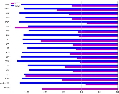
The values for 5% VaR and 5% ΔCoVaR for companies and Euro Stoxx 50 index are shown in Figure 4. The ΔCoVaR, which is the marginal risk contribution to the financial system, is achieved by calculating the difference between 5% CoVaR and 50% CoVaR for each company.
ΔCoVaR related to Euro Stoxx 50 is lower than that of Portuguese firms, which means that Portuguese stock market is more sensitive to major Portuguese firms than that of European companies.
As depicted in Figure 4, Corticeira Amorim and Novabase have the lowest ΔCoVaR, while EDP Renováveis and RENE have the highest marginal risk contribution respectively.
Similar to the discussed about CoVaR, there is no clear relationship between VaR and ΔCoVaR. A firm with high VaR might have a less than average ΔCoVaR, such as with Pharol in our analysis. In contrast, a firm with relatively low VaR can appear to have high ΔCoVaR, for which RENE is a good example.
Finally, we can conclude that considering VaR solely might not be sufficient and trustworthy for risk calculation due to interconnectedness of financial sectors leading to
31
spillover of risk from one sector to another and to the whole system. Therefore, systemic risk indicators such as CoVaR and ΔCoVaR should be taken into consideration.
Figure 4 – 5% VaR and 5% ΔCoVaR of PSI 20, Euro Stoxx 50, and PSI 20 listed firms
3.2. Portuguese banking system
In this section, we consider the Portuguese banking system in isolation. The period considered in this study starts from 03/04/2001 and ends at 31/07/2014, which is just before the resolution of Banco Espirito Santo (BES). The main consideration in choosing this period was the availability of data. Data for three Portuguese banks is available for a long enough period of time, which are Banco Espirito Santo (BES), Banco Comercial Português (BCP), and Banco Português de Investimento (BPI), considered as representative of thr Portuguese banking system, due to their weight on total assets (51%). Based on equation (26), daily return for banks are calculated. Taking returns of three banks together into account, we built the return of the Portuguese banking system. Now, we can study the effect of each bank on other banks and the system and the risk contribution of the system to each bank.
The VaR for the three banks and for their aggregate is given in Table I. It shows that among the three banks BCP had the highest VaR, while the aggregate VaR for the banking system had the lowest value at risk.
32 TABLE I
5%VAR OF PORTUGUESE BANKS AND BUILT FS
BES BCP BPI Portuguese FS
5% VaR -3.47% -3.94% -3.36% -3.24%
The same methodology explained in the previous section is used here to calculate CoVaR and ΔCoVaR. The estimated alpha, beta, CoVaR and ΔCoVaR resulted from regressing returns of individual banks on banking system aggregate, are given in Table II. Although BCP has the highest VaR, it has the lowest value for CoVaR. But it had highest ΔCoVaR again.
TABLE II
RESULTS OF REGRESSING THE SYSTEM ON AN INDIVIDUAL BANK
XSYSTEM |XBANK
Alpha Beta 5% CoVaR 5% ΔCoVaR
BCP -0.01424 0.6051 -3.81% -2.38%
BES -0.01975 0.6463 -4.22% -2.25%
BPI -0.02116 0.6222 -4.21% -2.09%
CoVaRSystem | bank i is the value at risk of the system (Pt banking system here)
conditional on having bank i at 5% level of its value at risk. For example, CoVaRSystem | BES equal to -4.21% means that the system 5% VaR is equal to -4.21% if VaR of BES is
at its 5% worst level.
ΔCoVaRSystem | Bank i, on the other hand, represents the risk contribution of bank i to
the system if the bank’s situation changes from normal situation to 5% VaR level. E.g. ΔCoVaRSystem | BES equal to -2.09% represents 2.09% decrease in 5% VaR of the system
due to change in risk condition of BES from median situation to 5% VaR.
Vice versa, the contribution of the system to individual bank is estimated by regressing each bank on the built Portuguese financial system. Table III indicated the estimated coefficients, CoVaR, and ΔCoVaR. BCP had the highest values for both CoVaR and ΔCoVaR. BES and BPI had similar ΔCoVaR values, but BES had a little bit higher CoVaR. It means BCP is more affected if the built banking system goes beyond
33
its 5% VaR level; however, BPI and BES showed more or less the same sensitivity to change in the built system return from its normal situation to 5% VaR level.
TABLE III
RESULTS OF REGRESSING INDIVIDUAL BANKS ON THE SYSTEM
XBANK|XSYSTEM
Alpha Beta 5% CoVaR 5% ΔCoVaR
BCP -0.01691 1.0384 -5.78% -3.36%
BES -0.02171 0.7131 -4.65% -2.31%
BPI -0.01999 0.7210 -4.43% -2.33%
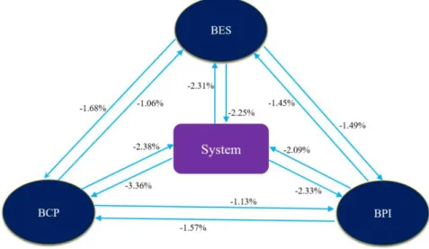
In addition, the effect of one bank’s risk on another is computable using the same approach, which means to quantify the risk that one bank adds to another in the case of being at its 5% VaR level. The regression coefficients are given in Appendix II. The CoVaRbank i | bank j, and the ΔCoVaRbank i | bank j estimations are given in table IV and table V, respectively. CoVaRbank i | bank j measures the VaR of bank i when bank j is at 5% VaR distress level, and ΔCoVaRbank i | bank j is the estimation of risk contributed to bank i through the movement of bank j from median state to 5% VaR distress state. Table IV indicates that BCP is relatively more sensitive to BES and BPI being at their 5% VaR level than vice versa. Table V shows that if BCP’s risk situation change from median state to 5% VaR level, it contributes relatively less risk to other banks than vice versa.
TABLE IV
RESULTS OF 5% COVAR OF BANK I CONDITIONAL ON BANK J
Bank i\ Bank j BCP BES BPI
BCP - -5.13% -5.10%
BES -3.88% - -4.47%
BPI -3.73% -4.24% -
As an example, CoVaRBCP | BES equals to -5.13% is the VaR of BCP conditional on BES being at its 5% distress level, and ΔCoVaRBCP | BES equals to -1.68% shows the decrease in BCP’s VaR is 1.68% if situation of BES changes from normal state to its 5% VaR.
34 TABLE V
RESULTS OF 5%ΔCOVAR OF BANK I CONDITIONAL ON BANK J
Bank i\ Bank j BCP BES BPI
BCP - -1.68% -1.57%
BES -1.06% - -1.45%
BPI -1.13% -1.49% -
Figure 5 summarize the results of ΔCoVaR for this section showing the risk contribution in Portuguese banking system.
Figure 5 – 5% ΔCoVaR relations between banks and the system
3.3. Risk linkage between international banks and the Portuguese banking system
The Portuguese banking system is not isolated from international banks and is interconnected to other banks of different parts of the world. In this section, we study the risk interaction between major banks of the world and the aggregate for the Portuguese banking system from 01/01/2008 to 31/07/2014 (just before the resolution of BES) to assess which banks contributed more to the risk of the Portuguese banking system, and which ones are more affected by it. The data for 47 international banks are considered. The list of 47 international banks can be found in Appendix III.
Again, the same methodology is used to calculate quantile regression coefficients, CoVaR, and ΔCoVaR. In this part, the daily returns of the market value of total assets of
35
the Portuguese banking system are regressed on that of individual international banks, and the risk contribution of each bank on Portuguese banking system is estimated. Besides, daily returns for the market value of total assets of the international banking system are calculated based on the total assets and the price-to-book value of equity of 47 international banks. Then, quantile regression coefficients, CoVaR, and ΔCoVaR from the regression of the Portuguese banking system on international banking system daily returns is estimated. The results are indicated in Table VI, showing that Banco Bilbao Vizcaya Argentaria, Intesa Sanpaolo, Danske Bank, ING Group, and Societe Generale are contributing more risk to the aggregate of the Portuguese banking system with ΔCoVaRs equal to -2.30%, -2.10%, -2.09%, -2.01%, and -2.01%, respectively. Not surprisingly, all of them are European banks.
Conversely, SLM Corp, Lloyds Banking, State Street Corp, Citigroup, and Barclays added less risk to Portuguese banking system with ΔCoVaRs equal to -0.01%, 0.04%, -0.18%, -0.19%, and -0.24%, respectively. Except for Lloyds Banking and Barclays, which are British banks, the remaining are US institutions. Therefore, the aggregate Portuguese banking system is more affected by European institutions than that of US or other countries.
The opposite risk direction, which is the risk contribution of Portuguese banking system to the international banks, is also analysed, and the result is presented in Table VII. It is detected that Banca Monte dei Paschi di Siena, Intesa Sanpaolo, UniCredit, ING Group, and Societe Generale are more sensitive to Portuguese banking system due to higher ΔCoVaRs equal to -1.82%, -1.81%, -1.50%, -1.43%, and -1.42%, respectively. In contrast, Commonwealth Bank of Australia, National Australia Bank, Nomura Holdings, Capital One Financial Corp, and Westpac Banking Corp were less sensitive and have lower ΔCoVaRs. Apparently, if the aggregate for the Portuguese banking system state changes from its median state to 5% VaR level, European banks are more affected than non-European banks. Especially, Australian banks are less affected than banks of other countries.
36 Table VI
RESULTS OF REGRESSING PORTUGUESE BANKING SYSTEM ON INTERNATIONAL BANKS
XPT BANKING|XINTERNATIONAL BANKS
Alpha Beta 5% CoVaR 5% ΔCoVaR
BBVA -0.032 0.584 -5.47% -2.30% ISP -0.034 0.432 -5.53% -2.10% DANSKE -0.036 0.525 -5.69% -2.09% INGA -0.034 0.388 -5.46% -2.01% GLE -0.036 0.422 -5.62% -2.01% SAN -0.034 0.497 -5.34% -1.94% UCG -0.034 0.324 -5.27% -1.84% STAN -0.038 0.362 -5.30% -1.53% EBS -0.037 0.271 -5.17% -1.50% CSGN -0.036 0.345 -5.08% -1.48% International system -0.039 0.483 -5.33% -1.42% NDA -0.038 0.342 -5.19% -1.39% WBC -0.040 0.462 -5.34% -1.37% BTO -0.036 0.404 -4.91% -1.32% SHBA -0.039 0.407 -5.16% -1.29% NAB -0.040 0.403 -5.28% -1.24% POP -0.035 0.268 -4.72% -1.15% DBK -0.039 0.254 -5.00% -1.10% SEBA -0.039 0.241 -4.97% -1.03% RY -0.040 0.376 -5.05% -1.01% CBA -0.040 0.347 -4.91% -0.94% BMO -0.041 0.339 -4.95% -0.91% BNS -0.041 0.323 -4.97% -0.89% CBK -0.038 0.144 -4.59% -0.82% TD CT -0.041 0.336 -4.83% -0.78% BNP -0.039 0.241 -4.65% -0.77% JT_8604 -0.041 0.174 -4.86% -0.77% CM -0.041 0.264 -4.85% -0.75% BBT -0.041 0.173 -4.79% -0.73% WFC -0.040 0.159 -4.72% -0.70% STI -0.041 0.120 -4.83% -0.69% GS -0.041 0.161 -4.72% -0.65% JT_8601 -0.041 0.142 -4.72% -0.61% JPM -0.040 0.141 -4.62% -0.61% SWEDA -0.040 0.161 -4.62% -0.60% BMPS -0.039 0.123 -4.47% -0.60% USB -0.041 0.153 -4.70% -0.60% BAC -0.040 0.109 -4.60% -0.58% PNC -0.041 0.127 -4.66% -0.55% COF -0.042 0.109 -4.71% -0.54%
37 Table VII
RESULTS OF REGRESSING INTERNATIONAL BANKS ON THE PORTUGUESE BANKING
SYSTEM
XINTERNATIONAL BANKS|XPT BANKING
MS -0.041 0.101 -4.57% -0.52% BK -0.041 0.103 -4.51% -0.42% UBSN -0.040 0.071 -4.37% -0.36% BARC -0.042 0.060 -4.41% -0.24% C -0.040 0.035 -4.23% -0.19% STT -0.041 0.040 -4.31% -0.18% LLOY -0.042 0.008 -4.22% -0.04% SLM UN -0.042 0.002 -4.21% -0.01%
Alpha Beta 5% CoVaR 5% ΔCoVaR
BMPS -0.044 0.437 -6.24% -1.82% ISP -0.042 0.436 -6.03% -1.81% UCG -0.049 0.360 -6.41% -1.50% INGA -0.048 0.344 -6.20% -1.43% GLE -0.042 0.341 -5.62% -1.42% CBK -0.053 0.341 -6.76% -1.42% BBVA -0.034 0.330 -4.76% -1.37% EBS -0.050 0.320 -6.36% -1.33% SAN -0.033 0.306 -4.62% -1.27% LLOY -0.042 0.306 -5.50% -1.27% DANSKE -0.036 0.302 -4.87% -1.26% STAN -0.040 0.292 -5.24% -1.21% BAC -0.053 0.284 -6.46% -1.18% BTO -0.028 0.283 -4.02% -1.18% POP -0.037 0.281 -4.89% -1.17% CSGN -0.039 0.241 -4.90% -1.00% NDA -0.039 0.222 -4.80% -0.92% SEBA -0.040 0.218 -4.95% -0.91% DBK -0.039 0.209 -4.78% -0.87% BARC -0.036 0.192 -4.40% -0.80% MS -0.050 0.182 -5.79% -0.76% BNP -0.030 0.181 -3.81% -0.75% STI -0.056 0.178 -6.37% -0.74% UBSN -0.048 0.174 -5.53% -0.72% SWEDA -0.035 0.166 -4.18% -0.69% SHBA -0.030 0.163 -3.67% -0.68% BK -0.039 0.154 -4.59% -0.64% International system -0.028 0.150 -3.40% -0.63%
38
3.4. International banks and BES risk contribution
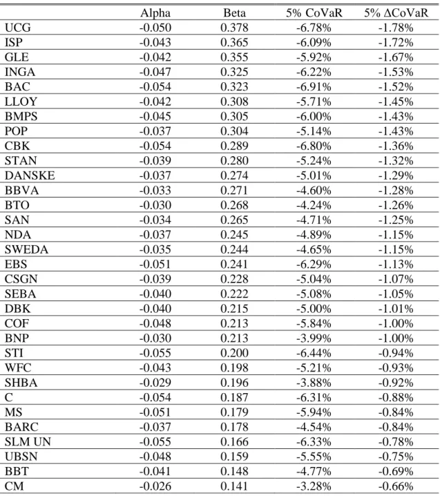
In this section, similar analysis as in section 3.4 is conducted, but instead of the aggregate for the Portuguese banking system, we focused on BES. The reason is to find banks that had more interconnectedness with BES during the same period considered in section 4. Since BES was resolved at the end of period, we can see which international banks are more affected, and which one added more risk to BES.
The results are given in Tables VIII and IX. Table VIII shows that BES contributed more risk to UniCredit, Intesa Sanpaolo, Societe Generale, ING Group, Bank of America Corp with ΔCoVaRs equal to -1.78%, -1.72%, -1.67%, -1.53%, and -1.52%, respectively. Conversely, Daiwa Securities Group, Nomura Holdings, Commonwealth Bank of Australia, National Australia Bank, and State Street Corp were less vulnerable to BES departure from its median state to its 5% VaR level due to their ΔCoVaRs equal to -0.06%, -0.33%, -0.35%, -0.40%, and -0.46%, respectively. As expected, BES added more risk to European banks than to other banks.
On the other hand, based on Table IX, Banco Bilbao Vizcaya Argentaria, Banco Santander, Societe Generale, ING Group, and Intesa Sanpaolo contributed more risk to
JPM -0.043 0.150 -4.89% -0.62% STT -0.043 0.147 -4.90% -0.61% C -0.055 0.143 -6.13% -0.59% CM -0.026 0.138 -3.22% -0.58% JT_8601 -0.041 0.135 -4.72% -0.56% SLMUN -0.055 0.134 -6.08% -0.56% BMO -0.026 0.127 -3.13% -0.53% GS -0.040 0.116 -4.44% -0.48% TD CT -0.022 0.109 -2.69% -0.46% WFC -0.042 0.107 -4.69% -0.45% PNC -0.043 0.104 -4.75% -0.43% RY -0.026 0.095 -2.96% -0.40% BNS -0.027 0.093 -3.04% -0.39% USB -0.038 0.085 -4.17% -0.35% BBT -0.041 0.082 -4.48% -0.34% WBC -0.029 0.068 -3.14% -0.28% COF -0.049 0.055 -5.18% -0.23% JT_8604 -0.044 0.053 -4.60% -0.22% NAB -0.030 0.040 -3.21% -0.17% CBA -0.027 -0.002 -2.69% 0.01%