Equity Valuation : Apple Inc intrinsic value and market price adjustment towards equilibrium

(1)

CATÓLICA-LISBON

Equity Valuation

Apple Inc intrinsic value and market price

adjustment towards equilibrium

Marco António Lourenço Madeira 03-06-2013

(2)

Marco Madeira Página 2

ABSTRATC

The main objective in this dissertation is to get an accurate estimate about Apple Inc intrinsic value in the end of the respective fiscal year (09/2012) using as valuation method the cost of capital approach. In addition, it is studied the long run relationship adjustment from market price towards respective fair value, using the error correction model.

Apple Inc intrinsic value was estimated to be equal to 533.912$ million taking into account 110.505$ million in cash. As a result, Apple Inc equity value per share was estimated to be equal to 568,48$. Additionally, the long run market price equilibrium would be equal to 470,96$ (assuming no changes in the intrinsic value).

(3)

Executive Summary

Company Apple Inc

Activity Designs, develops, and sells consumer

electronics, computer software and personal computers

Industry Consumer Electronics

Main Competitors Samsung

Price 09/2012 659,39$

Market Capitalization 616.449$ million

Price Target 09/2012 (Bloomberg) 780,17$

Main results presenting in this dissertation:

Intrinsic Firm Value 09/2012 533.912$ million Intrinsic Equity Value per share

09/2012

568,48$ Long Run Market Price Equilibrium 470,96$

(4)

1-Introduction

The main objective in this dissertation is to value Apple Inc. This company is well known corporation that designs, develops, and sells consumer electronics, computer software and personal computers. Its best-known hardware products are the Mac line of computers, the iPod music player, the iPhone smartphone, and the iPad tablet computer.

In September 2012, in the end of the company fiscal year, Apple Inc was a market capitalization equal to 616.449$ million, resulting in a market price per share equal to 659,39$. However, should we consider this market price as a fair value? If not, what price could be considered as fair and how long it would take for market price to adjust to the equilibrium price (intrinsic value)?

In order to get the estimative for the fair value we would have to present the fundamentals behind the valuation methods, comprehend them well, and therefore use and apply the valuation model which seem more accurate and properly suitable taking into account characteristics of this specific company.

In addition, to identify and be aware of the long term relationship between the intrinsic value and the market price we would need to use one specific econometric model, in particular, the error correction model. The main goal, is to know whether the market price is going to, fully or partial adjust to the intrinsic value, and how many time is going to last that adjustment to the equilibrium.

It is highly important to understand those questions. In fact, they can be very useful to get different insights regarding different problems. For example, it would be useful to be used for portfolio management; acquisitions analysis; public offerings; to identify the value main drivers; strategic decisions for the company, etc. In general, the main information that an investor can gather from the valuation analysis would be whether the market price is under or overvalued (compared that with other assets), or if it is possible to increase value of the company we are running or to be disposable to buy and running it instead.

(6)

2-Literature Review

There are “three main approaches to valuation: 1) the discounted cash flow valuation which relates the value of an asset to the present value of expected future cash flows on that asset; 2) relative valuation which estimate the value of an asset by looking at the pricing of comparables assets relative to a common variable such as earnings, operating cash flow, book value, or revenues; 3) contingent claim valuation which uses option pricing models to measure the value of assets that share option characteristics” (Damodaran 2002).

2.1 – Discounted Cash Flow Models

There are three main methods regarding discounted cash flow models: the Free Cash Flow to the Equity (FCFE) method that value just the equity stake in the business; the Dividend discount model (DDM) which is a particular case of the FCFE model; Free Cash Flow to the Firm (FCFF) method value the entire firm, which includes besides equity the other claimholders in the firm (debt holders); and finally the Adjusted Present Value (APV) method that value the firm in pieces, beginning with its operations and adding the effects on value of debt. Those methods can be described as follows:

a) Free Cash Flow to the Equity model(FCFE):

The general case to the Free Cash Flow to the Equity model is a function of the present value of expected FCFE in the future discounted at an appropriate discount rate, in this particular case, would be the cost of equity:

1

The Free Cash Flow to the Equity corresponds to the cash that is available to be paid out only for equity holders (stockholders) and include net income subtracted to reinvestment in capital expenditures, investment in working capital and net debt payments:

(7)

Marco Madeira Página 7 b) Dividend discount model (DDM)

( ) )! 1

“The dividend discount model is a particular case of FCFE equity method, assuming all cash flow to the equity is distributed as form of dividends between stockholders. In those conditions, there will be no future cash building in the firm, or said in another way, the changes in excess cash would be zero, since the cash that is available after debt payments and reinvestment needs is paid out to stockholders each period” (Damodaran 2002).

( ) )!

“If the company that we are valuing is expected to have a fixed management control because of the size, legal or market restrictions on takeovers, the appropriate valuation method should be the dividend discount model. If not, then we should useful to use the FCFE model” (Damodaran 2002).

c) Free cash flow to the firm model (FCFF):

The general case to the Free Cash Flow to the Firm method is a function of the present value of expected FCFF in the future discounted at the weight average cost of capital (debt holder plus equity holders):

# _{1 %}

The free cash flow to the firm (FCFF) is the sum of the cash flows to all claim holders in the firm, including stockholders, bondholders and preferred stockholders and incorporate the earnings before interest and taxes (EBIT), net out taxes, reinvestments needs in capital expenditures (CAPEX less depreciations) and working capital:

(8)

Marco Madeira Página 8 It is important to note, the cost of capital approach is an iterative process because the weight average cost of capital need as input the market values for debt and equity that ultimately can only be obtained performing the formula of the FCFF method initially. Nevertheless, this circular reasoning provides consistent results

Firms that either have very high leverage or are in the process of changing their leverage are best valued using the FCFF method. The calculation of FCFE is more difficult in these cases because of the volatility induced by debt payments (or new issues).

d) Adjusted present value model (APV):

The general case to the Adjusted Present Value model is a function of the present value of expected FCFF in the future discounted at the unlevered cost of equity added with present value of the tax shield benefits and subtracting the cost of borrowing.

V _{1 k}FCFFt

u t t ∞

t 1

VTS‐PV of expected bankruptcy costs

This tax benefit (VTS) is a function of the tax rate and interest payment of the firm discounted at a determined discount rate. “There are several theories regarding which are the fundamentals determinants behind this tax shield formula” (Fernández 2006). All those theories can be described as follows:

EFGHIJHKLH&EHJJNO PQNFOR: #,T " " U U ERNOV PQNFOR: #,T " " W W EHJJN PQNFOR: #,T 0 YKOOHV&ZOHLIJN PQNFOR: #,T " W" [ \NOLáLGN^ PQNFOR: #,T " " [ [

While the three approaches use different combinations of cash flow and discount rates, “they yield consistent estimates of value as long you use the same set of assumption in valuation” (Fernández 2006).

(9)

Marco Madeira Página 9 2.2 – Multiples Models

In relative valuation, “the value of an asset is derived from the pricing of comparable assets which are standardized trough the use of common variable such as earnings, cash flow, book value, or revenues” (Damodaran 2002).

In practice, relative valuation most often are computed using comparables through industry averages; multivariate regression models, and fundamentals equations which are equivalent to the discounted cash flows (requiring the same information and yielding the same results). It is important to note that multiples valuation can be done through cross sectional and time series comparisons.

The main relative multiples are the following methods: price earnings ratio; price to book ratio; price to sales ratio and finally enterprise value to EBITDA ratio. The determinants behind each of these multiples may be explained as follows:

a) The price-earnings multiple is the ratio of the market price per share to the earnings per share. The fundamentals behind this ratio can be described as follows:

/ ` a " 1 b_b c

c

b) The price to book ratio is computed by dividing the market price per share by the current book value of equity per share. The determinants are:

/*# de " ` a " 1 b_b c

c

c) The price to sales ratio can be described as:

/T f ! g b " ` a " 1 b_b c

(10)

Marco Madeira Página 10 d) The enterprise value to EBITDA multiple relates the total market value of the firm, net of cash, to the earnings before interest, taxes, depreciation, and amortization of the firm. The determinants of the enterprise value to EBITDA multiple can be register as:

#/ *+, 1 *+, 1

d ( ! *+,

% bc

The main limitations on multiples are the following: 1) they are difficult to use to value firms with no obvious comparables, 2) with little or no revenue and with negative earnings, easy to misuse and control especially when are used comparables, 3) biased analyst can choose a group of comparables to confirm their biased, 4) the definition of what is comparable is subjective.

2.3 – Option Model

“Contingent claim or option is a claim that pays off only under certain contingencies. If the value of the underlying asset exceeds a pre specified value for a call option or is less than a specified value for a put option” (Damodaran 2002).

The well known formula used in option valuations is the method established Black and Sholes:

# fa g h ff T ) i jk ₎_l

mh : ) ln oTip q rl

2 t

r√ ; )l ) r√

Limitations on option method may be described as: 1) the assumptions made about constant variance and dividend yield, which are not contested for short run options are much different when long life time; 2) when underlying assets is not traded, the inputs for valuing cannot be extracted and have to be estimated, consequently, the option method become less reliable.

(11)

Marco Madeira Página 11 Threat of Rivalry (Super High) Threat of Suppliers (Low) Threat of Buyers (Moderate) Threat of Substitutes (Moderate) Threat of Entry (Low) Size (High) Growth (High) Margin (Moderate) Risk (High)

3-Methodology and Results

3.1- Industry analysis

Apple Inc is a company that is operating in a consumer electronics and personal computer industry. This sector is very competitive, with aggressive competitors always trying to producing better electronics devices with more competitive prices.

According to this, we may say that major threat came from the competitors, in particular from Samsung.

(12)

Marco Madeira Página 12 $0 $20.000 $40.000 $60.000 $80.000 $100.000 $120.000 2000 2001 2002 2003 2004 2005 2006 2007 2008 2009 2010 2011 2012 Excess marketable securities

3.2- Asset, liabilities and equity measurement

We are going to begin our analysis, looking for Apple Inc financial statements during the period from 09/2000 to 09/2012 (fiscal year ends in September). The main goal, is to account, classified and compared the assets, liabilities and equity values during the period in analysis according to what was presenting in the balance sheet statement (appendix 1).

In this sense, trough a historic analysis on Apple Inc we may take the following conclusions regarding the assets side: 1) their assets changed from 6.803$ million to 176.064$ million which represent an increase of +169.261$; 2) noncurrent assets changed +25.699$ million and are composed by 15.452$ million in tangible assets (plants, equipment, land, and buildings); 5.359$ million in intangible assets (patents, trademarks and goodwill) and 5.478$ million in other noncurrent assets; 3) current assets had a variation of + 36.679$ million and include 791$ million in inventory (raw materials, work in progress, and finished goods), 10.930$ million in account receivables and 10.746$ million in operating cash, 14.220$ million in other current assets; 2.583$ million in deferred tax assets; 4) excess cash and marketable securities (financial investments) is valued at 110.505$ million and correspond to an increase of + 106.883$ million (as you can see in figure 1).

(13)

Marco Madeira Página 13 $0 $50 $100 $150 $200 $250 $300 $350 2000 2001 2002 2003 2004 2005 2006 2007 2008 2009 2010 2011 2012 Debt

In the another side of the balance sheet, liabilities and equity may be described as follows: 1) current liabilities had a variation of + 36.609$ million and is composed by 0$ million in short term debt, 21.175$ million in account payable and 17.367$ million in other current liabilities; 2) 16.664$ million in other noncurrent liabilities, 3) 2.648$ million; 4) in deferred taxes; 4) 0$ million in long term debt. It is important to note that the company doesn’t have any financial debt since 2004 (as you can see in figure 2); 3) equity shareholders is valued at 118.210$ million representing a cumulative 16.422$ million in proceeds received by the firm from equity that was issued and from the sum of all retaining earnings in the amount of 101.788$ million (taking into account adjustments from paid dividends and other comprehensive income items).

Using the same accounting figures, we can look into the balance sheet in a different perspective. Instead of divide Apple Inc in assets, liabilities and equity, we organize the balance sheet dividing the items by the following categories: 1) sources of funds obtained by the firm; 2) applications of those funds (appendix 2)

Thus, if we sum up the equity plus short term and long term debt we get the 118.210$ million in total funds representing a + 113.803$ variation during the period in analysis Those funds were applied -1.855$ million in operating working capital (2.548$ million), 18.956$ million in operating invested capital (+17.726$ million), -11.186$ million in other current assets, net of other noncurrent liabilities (--11.186$ million), -65$ deferred tax assets, net of deferred tax liabilities (+0$ million), and finally 110.505$ million in excess cash and marketable securities (+106.883$ million).

(14)

Marco Madeira Página 14 -$20.000 $0 $20.000 $40.000 $60.000 $80.000 $100.000 $120.000 $140.000 $160.000 $180.000 2000 2001 2002 2003 2004 2005 2006 2007 2008 2009 2010 2011 2012 EBIT Revenues

3.3- Measuring earnings, profitability, risk and market ratios

It is time to move on, and ask whether the firm is being a profitable or not? In order to accomplish that task we use the income and cash flow statements (appendix 3 and 4) during the time interval 2000 to 2012. It was concluded that Apple Inc has been presenting positive

earnings with a growing pattern. As you may see in figure 3, revenues had increased from 7.983$

million to

156.508$million; EBIT moved from 620$ million to 55.241$ million; and finally, net income had changed from 786$ million to 41.733$ million.

However, those conclusions just allow us to confirm that Apple Inc is been profitable in absolute term. In order to get a full picture, we should also take into account how much money is invested in the company to see whether the firm is being profitability in relative terms. In this sense, we are going to take a look on main financial ratios of the company (appendix 5).

This analysis can be done using the return on equity (ROE) which is determined by the return on capital (ROC), debt to equity (D/E) and after tax interest rate. Using those fundamentals we understand that changes in ROE are caused by variations in ROC and in leveraged ratio.

ROE ROC D_{E {ROC‐i 1‐t }} Figure 3

(15)

Marco Madeira Página 15 0,000 0,010 0,020 0,030 0,040 0,050 0,060 0,070 0,080 0,090 0,00% 5,00% 10,00% 15,00% 20,00% 25,00% 30,00% 35,00% 40,00% 2000 2001 2002 2003 2004 2005 2006 2007 2008 2009 2010 2011 2012 Return on capital Debt to equity ratio

0,00% 5,00% 10,00% 15,00% 20,00% 25,00% 30,00% 0,000 0,500 1,000 1,500 2,000 2,500 2000 2001 2002 2003 2004 2005 2006 2007 2008 2009 2010 2011 2012

Capital turnover ratio After tax operating margin In practice, during

the time interval 2000-2012, the ROE from Apple Inc has changed from 16.71% to 35.79%. This positive evolution was caused by: increased in return on capital from 15.91% to 35.79%; change in debt to equity from 0.073 to 0; negative

variation regarding after tax book interest rate from 5.04% to 0% (as you can see in figure 4)

It is also important to note that return on capital is determined by the after tax operating margin and capital turnover ratio.

de g , ~ O b M b " f Ta ( R

In this sense, the return on capital increased due to positive variations on after tax operating margin from 8.78% to 27.03% in spite of the negative changes in capital turnover ratio from 1.811 to 1.324 (as you can see in figure 5)

Concluding, we comprehend that the positive and growing pattern on Apple Inc return on equity (ROE) has been largely influenced by the return on capital, in particular, by the after tax operating margin.

Figure 4

(16)

Marco Madeira Página 16 0,000 0,500 1,000 1,500 2,000 2,500

Quick ratio Current ratio

-70,0 -60,0 -50,0 -40,0 -30,0 -20,0 -10,0 0,0

Required financing period About risk analysis,

there are two frequent measures: current ratio and quick ratio. In Apple Inc case (as you can see in figure 6) both ratios were well above 1 which indicates that, as a firm, they have less obligations coming due in the next year than assets it can

expect to turn in cash. This result implies low liquidity risk through the period 2000-2012.

Another way to measure liquidity is using turnover ratios on receivables; payables; and inventory. Those ratios represented the speed with which the firm turns account receivables into cash; inventory into sales; and payables into purchases (expressed in terms of number of days). If we sum up the days account held with day’s account receivables subtracting with days account payables we get the required financing period.

As you can observe in figure 7, during the period in analysis (2000-2012), Apple Inc has presented a negative required financing period which means the company hasn’t asked any short term borrowing implying low liquidity risk, and confirming the liquidity ratios mentioned before.

Figure 6

(17)

Marco Madeira Página 17 $0 $100.000 $200.000 $300.000 $400.000 $500.000 $600.000 $700.000 2 0 0 2 2 0 0 3 2 0 0 4 2 0 0 5 2 0 0 6 2 0 0 7 2 0 0 8 2 0 0 9 2 0 1 0 2 0 1 1 2 0 1 2 Market Capitzalization 0,000 0,010 0,020 0,030 0,040 0,050 0,060 0,070 0,080 0,090

Debt to equity ratio

Regarding default risk which quantifies the long term solvency and analyze the firm capacity to meet interest and principal payments in the long term, we may conclude that Apple Inc

has no default risk. Since 2004, the interest coverage ratio and the debt ratios were equal to zero (figure 8) meaning Apple Inc has no debt payments since then. Therefore, the default risk, as stated above, may considered almost nonexistent.

The upbeat

evolution on earnings and return on equity, have influenced Apple Inc market price which had increase from 14, 72$ in 2002 to 659, 39$ in 2012 corresponding to an positive variation of 644,67$ (43,79% average annual return).

Moreover, the firm has register an increase in market capitalization (figure 9) from 5.316$ (1.298 times equity book value) million to 616.449$ million (5.334 times equity book value). Today, Apple Inc has been valued in the market 115,96 times more than twelve years ago.

Figure 8

(18)

Marco Madeira Página 18 3.4- Firm valuation

Now, it is time to start Apple Inc valuation. The value of the firm can be estimated using in practice all methods stated before (discount cash flow, multiples and options). However, the more suitable would be the discounted cash flow models because we are valuing unique assets which is Apple Inc, with proved capacity to generate cash flow for a long time horizon (to perpetuity). Of course, this method only makes sense assuming that markets make mistakes but correct themselves them over time.

But, which discount cash flow method should be used? Well, for firms with stable leverage, debt ratios that are not expected to change during the period of valuation. Under these circumstances, it would be equal to use the FCFE, FCFF or APV. However, in this particular case, we are going to apply the cost of capital approach (FCFF) on Apple Inc for the reason that: first, as a firm, they been presenting stable leverage during the last few years (as we have see before); second, latter we are interested to understand the impact of changes in the debt ratio on the firm value.

Therefore, we are going to base our valuation on the cost of capital approach which values the company through the present value of expected free cash flow to the firm discounted at the weight average cost of capital.

V _{1 WACC}FCFFt _t

t ∞ t 1

In addition, it would be useful to divide it in three stages: 1) high growth phase; 2) transition phase for gradual adjustments not just of growth rates but also risk characteristics, return on capital, and reinvestment targets towards stable growth levels; 3) stable growth phase (assuming economic full employment)

V FCFFt ‚1 WACChg…t t n1 t 1 FCFFt 1 WACCtr t t n2 tn1 1 FCFFn 1/ WACCsg‐gn 1 WACChg n

(19)

Marco Madeira Página 19 The first stage, the high growth period would have duration of three years. This short period of time represents Apple current growth revenues momentum conditioned by the weakening competitive advantage which has been decrease abruptly due to fierce competition (SAMSUNG) that have been producing new products with similar quality with very competitive prices. In this sense, it is expected a short time high growth period, proceeded by a ten years transitory period until reach the stable growth under a full employment conditions.

High growth period:2013‐2015 3years Transitory period:2015‐2025 10 years

Stable period:Š2025 Perpetuity

Now, it is time to applied the FCFF method and forecast the inputs required to accomplish that task.

3.4.1- WACC for high growth period

First of all, in order to estimate the value, we need to compute the discount rates that reflect the riskiness of the cash flow. In particular, we would need to determine the cost of debt (compute the default spread for the default risk in the debt), and the cost of equity (find out the risk premium for equity risk).

WACC D/V "After Tax Cost of Debt Cost of Equity " E/V

In order to calculate the equity risk premium we need to use the capital asset pricing model (CAPM). In practice, we would use three inputs:

Risk-free asset - defined to be an asset for which the investor knows the expected return with certainty for the time horizon.

Risk premium - the premium demanded by the investors for investing in the market portfolio.

Beta - defined as the covariance of the asset divided by the market portfolio measure the risk added to an investment to the market portfolio.

(20)

Marco Madeira Página 20 For risk-free rates there are several conditions that have to be met: 1) there can be no default risk; 2) no reinvestment risk; 3) should be consistently estimated with cash flow. According to this, the only way to follow those conditions is to use debt issued with the following characteristics:

Issued by the US government - they have effective control and authority to print currency. Therefore, in theory, the government securities have no risk because, in theory, they are able to assure full debt payments. The maturity used is going to be equal to 10-years, in order to match up

the duration of the risk free rate with the duration of twelve years cash flow projection in this study.

Taking into account that US economy has a stable inflation, we are going to use a nominal risk free rate (consistently with nominal cash flow estimation).

Therefore, we decided to apply the nominal US-10 YEAR Bond as risk free rate.

Risk Free Rate rf 1,63%

The risk premium, in practice, is estimated looking at the current difference between the expected market risk for SP&500 and the risk free rate. In this case, we get the following risk premium:

Risk premium E• RM ‐rfŽ 10,31%‐1,63% 8,68%

Finally, as input in CAPM, we also need to measure of a firm exposure to market risk in the form of betas. The conventional approach for estimating the beta of an investment is a regression of returns on the investment against the return on a market index (SP&500). In this particular case, Apple Inc had the following beta:

(21)

Marco Madeira Página 21 In addition, we calculate the fundamental betas taking into account the degree of operating leverage or firm financial leverage. To estimate the unlevered beta, it is used an historical average marginal tax rate of 25% and an historical average debt to equity equal to 0.

βU βCorrent

&1 1‐t oaverage debt_equityp'

0,978

{1 1‐0,25 0 } 0,978

The unlevered beta for Apple was equal to 0,978. The levered beta is going to depend on the unlevered beta (already calculated) and on the market value for debt and equity.

Debt market value 0$ million Equity market value 630.586$

The debt to equity in market terms is equal to:

Debt to equity market value 0

Taking into account those calculations, we can estimate the beta levered as follows:

βl βU" &1 1‐t q_{equityt' 0,978"{1 1‐0,25 0 } 0,978}debt

Finally, having estimated the risk free rate, the risk premium and the beta, we are able to get the expected return from investing in equity. For Apple case, the cost of equity would be equal to:

(22)

Marco Madeira Página 22 The other parameter is the cost of debt which can be determined by the following variables: 1) risk free rate; 2) the default risk and spread; 3) tax advantages associated with debt.

After tax cost of debt {rf default spread}"{1‐t}

So, we need to compute a synthetic rating in order to find which default to address. In this case, as we have seen before, Apple Inc has no debt and consequently no interest payments. The interest coverage ratio is zero, implying a debt classification as AAA rating.

Debt Rating: AAA

Thus, in this particular case, with a AAA rating the default spread is going to be 0,40%, the risk free rate equal to 1,63% and the marginal tax rate would be to 25% (taking into account the historical record). According to this, the after tax cost of debt may be forecasted as:

After tax cost of debt {1,63% 0,40%}"{1‐0,25} 1,53%

Finally, we are able to estimate the weight average cost of capital that reflect their market value proportion of debt and equity multiplied respectively by the cost of equity and after tax cost of debt. In fact, the debt weight would be zero and equity weight should be 1 reflecting the current capital structure of the company in market terms.

The cost of equity and the after tax cost of debt should be equal to 10,12% and 1,53%, respectively. Therefore, the cost of capital (WACC) would be equal to 10,12%.

WACC 0"1,53% 1"10,12% 10,12%

It is important to note, all detail and historical values regarding risk parameters are presented in appendix 6.

(23)

Year R&D Expense Unamortized portion Amortization this year

Current $3.381 1 $3.381 $0 -1 $2.429 0,8 $1.943 $486 -2 $1.782 0,6 $1.069 $356 -3 $1.333 0,4 $533 $267 -4 $1.109 0,2 $222 $222 -5 $782 0 $0 $156 -6 $712 -0,2 -$142 $142 -7 $535 -0,4 -$214 $107 -8 $489 -0,6 -$293 $98 -9 $471 -0,8 -$377 $94 -10 $446 -1 -$446 $89 -11 $430 -1,2 -$516 $86 -12 $380 -1,4 -$532 $76 -13 $314 -1,6 -$502 $63 0 $0 0 $0 $0 0 $0 0 $0 $0 0 $0 0 $0 $0 0 $0 0 $0 $0 0 $0 0 $0 $0 0 $0 0 $0 $0 0 $0 0 $0 $0 $4.125 $2.242 $3.381 $2.242

(Apple Inc) - R&D Converter

Expenditure on asset in current year = Amortization of asset for current year = Value of Research Asset = 3.4.2- FCFF for high growth period

As it was presented before, the value of a firm using the FCFF method need as input the expected cash flows. To compute the expected cash flows we need two parameters: the expected reinvestment rate and the expected growth in after tax operating income.

FCFFt EBITt‐1{ 1‐t 1 Growth ratet ‐Reinvestment Ratet}

In order to find the expected reinvestment rate we are going to use the latest (2012) value about the following components: net capital expenditure; investment in working capital; and finally research & development expenses which need to be capitalized and adjusted on EBIT and assets (as you can see in table 1).

(24)

Marco Madeira Página 24 In this sense, it is important to note that current after tax operating income must be adjusted adding up to the current R&D expenses and subtracting the amortization of the research asset taking into account supplement calculations (using Damodaran converter template). In result, we would get 42.088$ million operating earnings after taxes.

Adjusted after tax EBIT2012 $million 40.949$ 3.381$‐2.242$ 42.088$

Therefore, the current year R&D expenses (3.381$ million) added to the current capital spending (changes in gross property, plant and equipment plus changes in intangible assets) equal to 11.046$ million, less current amortization (2.242$ million) and depreciation (2.444$ million), in conjunction with a current decrease in working capital of 722$million, we estimate an adjusted reinvestment rate for the firm of 21,43%. In the process, it is assumed that the expected reinvestment rate would be equal to the previously (2012) assuming the company investment spending policy is going to continue as in the past.

Adjusted Reinvestment Rate RR 14.427$‐4.686$‐722$ _42.088$ 21,43%

The other input is the expected growth rate for operating earnings (EBIT). According to the fundamentals, a firm growth is determined by how much is reinvested into new assets and the quality of those investments. You can relate growth in operating income to total reinvestment made into the firm and the return earned on capital invested.

Growth rate g RR "ROC

To estimate the return on capital, we estimated the value of the research asset at the end of the previous year (2012) added it to the book value of equity. We assume that the previous accounting return on capital is a good measure of the return earned on existing investments and this return is a good proxy for future returns that will be made on future investments.

(25)

Return on Capital Reinvestment Rate EBIT growth EBIT EBIT after Taxes Reinvestment FCFF

2012 $55.241

F 2013 34,40% 21,43% 7,37% $59.313 $44.485 $9.532 $34.953

F 2014 34,40% 21,43% 7,37% $63.686 $47.764 $10.235 $37.530

F 2015 34,40% 21,43% 7,37% $68.381 $51.286 $10.989 $40.296

(Apple Inc) - Free Cash Flow to the Firm

Therefore, the return on capital for the firm is forecasted as:

Return on capital ROC _{118.210$ 4.125,40$ 34,40%}42.088$

In this sense, the expected growth in operating income is a product of the reinvestment rate and the quality of the investments measured as the return on capital.

Growth rate g 21,23% "34,40% 7,37%

As a result, take into account those calculation, we can estimate the Free Cash Flow to the Firm for the first the three years high growth phase (as you may see in table 2).

FCFF2013 55.241$ "{ 1‐0,25 1 7,37% ‐21,43%} 34.953 million

FCFF2014 59.313"{ 1‐0,25 1 7,37% ‐21,43%} 37.530 million

FCFF2015 63.686"{ 1‐0,25 1 7,37% ‐21,43%} 40.296$ million

(26)

Marco Madeira Página 26 0,00% 1,00% 2,00% 3,00% 4,00% 5,00% 6,00% 7,00% 8,00% Growth 3.4.3- WACC and FCFF for stable growth period

Firms that reinvest substantial portions of their earnings and earned excess returns on these investments should be able to grow at high rates. But as firms grows, it becomes more difficult for it to maintain a high growth and it eventually will grow at a rate less than or equal to the growth rate of the economy in which it operates.

In this particular case, we are going to consider the stable growth as the annual average (2000-2012) nominal US gross domestic product equal to 4,08% (appendix 7).

Stable growth rate 4,08%

In the figure 10 may find the representation of the transition on stable growth rate from 7,37% (high growth period) to 4,08% (stable growth period).

In this sense, as firm move from high growth to stable you would expect stable growth firms to have average risk, use more debt, lower or no excess returns. Therefore you should adjust each of these variables to be consistent with the stable growth rate: cost of equity, cost of debt, return on capital, debt ratio, reinvestment rate.

(27)

Marco Madeira Página 27 0,965 0,970 0,975 0,980 0,985 0,990 0,995 1,000 1,005 Current Beta

Regarding the cost of equity, we need to adjust the beta; the risk free rate and the expected market return on SP&500.

As a result, if we assume the company have less exposure to market risk, then beta parameter would become closer to 1 Thus, the beta parameter would move from 0,978 in high stage period to 1 in stable period (as you can observe in figure 11)

In respect to the risk free rate, we would consider the interest rate in a full employment economy. In order to get that interest rate, we use an economic equation known as Taylor rule.

U Ÿ ¡ ¡¢ l £ £¤k¥

Through a regression (appendix 8), using the historical risk free rate, output gap and inflation differential (appendix 7), we would get the following parameters:

U 0,0363 0,000040 " ¡ ¡¢ 0,3561 " £ £ ¤k¥

In result, if we assume an economy in full employment, the actual GDP would be equal to potential GDP and actual inflation would be equal to the targeted inflation. Therefore, the risk free rate for stable growth would be:

rf 3,63%

(28)

Marco Madeira Página 28 9,95% 10,00% 10,05% 10,10% 10,15% 10,20% 10,25% 10,30% 10,35% 10,40% 10,45% 0,00% 0,50% 1,00% 1,50% 2,00% 2,50% 3,00% 3,50% F 2013 F 2014 F 2015 F 2016 F 2017 F 2018 F 2019 F 2020 F 2021 F 2022 F 2023 F 2024 F 2025

Aftet Tax Cost of Debt Cost of Equty

In respect to the expected return on SP&500, we would consider the arithmetic average regarding the period from 2000 to 2012 (appendix 6).

E RM

¦¦¦¦¦¦¦¦ 10,41%

Therefore, resulting on those risk transformations, we may compute the cost of equity on stable phase as:

Cost of equitystable growth 3,63% 1" 10,41%‐3,63% 10,41%

Regarding debt costs, in theory, as firms matures, their debt capacity increase but the question whether debt ratio should be move towards a more sustainable stable growth level depended on managers views on debt. In this particular case, we don’t have any information’s about managers will regarding changes in their financing policy. Therefore, it is safer to leave level of debt ratio at exiting levels. In this case, would determine a zero debt ratio for the stable period.

After tax cost of debtstable growth {3,63% 0,40%}"{1‐0,25} 3,02%

In the following figure 12, we may see the evolution on cost of equity and after tax cost of debt resulting on the parameters modifications from high period to stable phase.

(29)

Marco Madeira Página 29 0,00% 5,00% 10,00% 15,00% 20,00% 25,00% 30,00% 35,00% 40,00% WACC ROC

Thus, we are able to estimate the weigh average cost of capital for the stable growth. In this case, the cost of capital would be equal to 10,41%.

WACCstable growth 0"3,02% 1"10,41% 10,41%

In stable growth, as it was stated before it is more difficult to maintain excess returns eternally. Thus, we are going to assume that, in the stable phase, the return on capital is equal to the cost of capital corresponding to a situation where the company is unable to perform excess returns. .

ROCstable growth WACCstable growth 10,41%

The return on invested capital (ROC) was always higher than the weight average cost of capital (WACC). However, this growing patter would only continue until 2015, which represent the last year of the high growth phase. After then, it is expected that Apple Inc economic value added continue to be positive but with a downward pattern until reach the stable period in 2025. This dynamic is well represented in the figure 13.

(30)

Marco Madeira Página 30 0,00% 5,00% 10,00% 15,00% 20,00% 25,00% 30,00% 35,00% 40,00% 45,00% F 2013 F 2014 F 2015 F 2016 F 2017 F 2018 F 2019 F 2020 F 2021 F 2022 F 2023 F 2024 F 2025 Reinvestment Rate $0 $10.000 $20.000 $30.000 $40.000 $50.000 $60.000 F 2013 F 2014 F 2015 F 2016 F 2017 F 2018 F 2019 F 2020 F 2021 F 2022 F 2023 F 2024 F 2025

Free Cash Flow to the Firm

Having fixed the growth rate on after tax operating income and return on capital equal to weight average of capital, the reinvestment rate must be determined in way that not violates those two conditions on growth and return on capital settled before.

RRstable growth _{10,41% 39,20%}4,08%

This figure 14 represents the evolution on reinvestment rate during the period from transition to stable

phase. As you can see, the reinvestment rate corresponds to a growing pattern in order to compensate the decrease in the return on capital and at same time to be consistent with the expected growth rate.

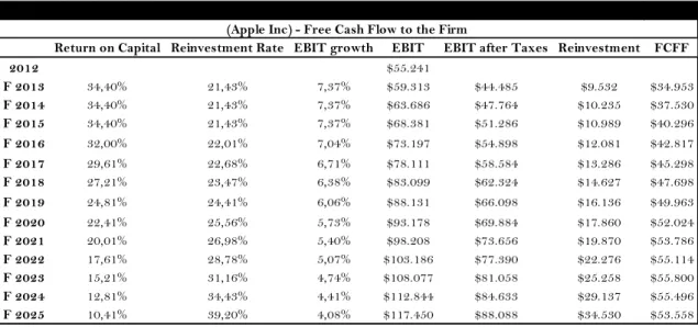
In result of the assumptions made regarding growth and risk during the different periods in analysis, we get the following figure 15. It is represented the forecast for Apple Inc Free Cash Flow to the Firm (appendix 9). It is observed an increase from 34.953$ million in 2012 to 53.558$ million in 2025.

Figure 14

(31)

Marco Madeira Página 31 $0 $20.000 $40.000 $60.000 $80.000 $100.000 $120.000 $140.000 $160.000 $180.000 $200.000

High growth Transition Stable growth Sources of value

Return on Capital Reinvestment Rate EBIT growth EBIT EBIT after Taxes Reinvestment FCFF

2012 $55.241 F 2013 34,40% 21,43% 7,37% $59.313 $44.485 $9.532 $34.953 F 2014 34,40% 21,43% 7,37% $63.686 $47.764 $10.235 $37.530 F 2015 34,40% 21,43% 7,37% $68.381 $51.286 $10.989 $40.296 F 2016 32,00% 22,01% 7,04% $73.197 $54.898 $12.081 $42.817 F 2017 29,61% 22,68% 6,71% $78.111 $58.584 $13.286 $45.298 F 2018 27,21% 23,47% 6,38% $83.099 $62.324 $14.627 $47.698 F 2019 24,81% 24,41% 6,06% $88.131 $66.098 $16.136 $49.963 F 2020 22,41% 25,56% 5,73% $93.178 $69.884 $17.860 $52.024 F 2021 20,01% 26,98% 5,40% $98.208 $73.656 $19.870 $53.786 F 2022 17,61% 28,78% 5,07% $103.186 $77.390 $22.276 $55.114 F 2023 15,21% 31,16% 4,74% $108.077 $81.058 $25.258 $55.800 F 2024 12,81% 34,43% 4,41% $112.844 $84.633 $29.137 $55.496 F 2025 10,41% 39,20% 4,08% $117.450 $88.088 $34.530 $53.558

(Apple Inc) - Free Cash Flow to the Firm

In table 3, we resume the forecasted FCFF as follows:

Finally, we would get the following estimation for the value of the Apple Inc operating assets for the end of 2012 fiscal year (appendix 10).

Value of the §irm operating assets 423.407$ million

The following figure 16 summarizes the different source of operating value for, high growth, transitory period and stable growth. In the graph we can the high growth contribute with 21,84% of the value, the transition phase represent 43,82% and finally the stable growth correspond to 34,34% of the final value of operating assets:

Figure 16 Table 3

(32)

Marco Madeira Página 32 6,00% 8,00% 10,00% 12,00% 14,00% 16,00% 18,00% $200.000 $250.000 $300.000 $350.000 $400.000 $450.000 $500.000 0% _10% _20% _30% _40% _50% _60% _70% _80% _90% 100%

Firm Value WACC

3.5- Effects of leverage on firm value (operating assets)

In order to understand the relationship between the cost of capital and the optimal capital structure, we rely on the relationship between firm value and the cost of capital. If we want to maximize firm value, we may accomplish it, trough minimization the cost of capital. In practical term the effect on firm value of changing the capital structure is isolated by keeping the operating income fixed varying only the cost of capital

First, we estimate different cost of equity to each debt ratio through changes in the levered beta according to those debt ratios. Second, we estimate the cost of debt taking into account the default risk depending on the interest coverage which depends on the level of debt payments. Therefore, once have estimated cost of equity and cost of debt to each level, we weight the in proportion used each to estimate the cost of capital (all calculations may be observed in appendix 11).

In result, as you can see in the figure 17, the firm value and the cost of capital have opposite directions. The firm value growth as you increase debt and reduce the cost of capital until reach the debt ratio equal to 40%. This point can be considered as the optimal debt level which maximize firm value as follows 451.379$ million. After then, more debt, imply a higher weight average cost of capital (WACC) and, consequently, a lower value for Apple Inc operating assets.

(33)

Marco Madeira Página 33 3.6- Estimating equity value per share

Once the value the operating assets are valued, you can add the value of the cash and marketable securities and subtract the debt to arrive at the equity value.

Equity 423.407$ million ‐0million $ 110.505$ million 533.912$ million

Taking into account, 939.200 million outstanding shares, we would get a final value for the equity share for the end of the fiscal year of Apple Inc (09/2012):

Equity value per share _{939.200 million oustanding shares 568,48$}533.912$ million

When compared this value estimation with Bloomberg Terminal target for the same date (09/2012) we would get a difference of 211,69$.The average equity share price target for Apple Inc taking into account Bloomberg analytical recommendations was equal to 780,17$.

The reasons why there is differences could be related to the following issues: 1) the majority of investment banks publish their valuations using multiples methods; 2) the value depend much on the individual investor opinion about several assumptions such as: reinvestment rate, return on capital, marginal tax rate and interest rates (as you are going to see latter).

(34)

Marco Madeira Página 34 3.7- Comparative analysis with Investment Bank report

Besides, we try to compare our valuation with JPMorgan report (appendix 19) from 26/10/2012 (the following date after the end of the fiscal year 2012). According to this report, the price target is equal to 770$ which means a difference of 202$ comparing with our valuation. Those fundamental differences in those targets are caused mainly by three reasons: 1) JPMorgan report use as valuation the multiple method; 2) the assumption about EBIT growth are divergent; 3) the time horizon is completely different.

As you may see in table 4, JPMorgan provide projections just for three year horizon and expect an EBIT increase from 55.241$ million in 2012 to 67.053$ million in 2014. In our valuation, as seen before, the time horizon is equal to thirteen years and the EBIT growth is expected to move from 55.241$ million to 63.686$ million which represent -3.367$ million than JPMorgan estimative.

(35)

Marco Madeira Página 35 -$25 -$20 -$15 -$10 -$5 $0 $5 $10 Marginal Tax Rate ROC RR Expected Market Risk Risk Free Rate Stable Growth Beta

Sensitivity on Equity Value per Share

3.8- Sensitive analysis on equity value per share

It is important to take a critical perspective on the estimated value. Therefore, we take a sensitive analysis (appendix 12) to understand the impact in the equity value per share of 1p.p (percentage point) change in several assumptions as: return on capital (ROC), reinvestment (RR), marginal tax rate (t), risk free rate, expected market risk, stable growth (g) and beta.

As you can see in figure 18, 1 p.p change in return on capital and reinvestment rate have positive impact of approximately 5$ in the equity valuation. Of course, if we increase the quality of the investments or the reinvestment rate we would get higher cash flows and therefore higher equity estimation.

In one hand, an increase of 1pp in expected market risk, beta and risk free rate increase the cost of capital and therefore had a negative impact on the valuation. In another hand, positive changes in the marginal tax rate have two effects: decrease the amount of free cash flow and decrease the cost of capital. In this case, the first effect is more powerful (-6,02$).

Finally, changes in 1 pp in stable growth had a negative impact in the equity value per share because we assume the return on capital (10,41%) is fixed in stable period and therefore to increase growth the company need to reinvest more. In this sense, we would get a lower free cash flow and consequently a lower equity valuation.

(36)

Marco Madeira Página 36 3.9- Market price adjustment towards equilibrium

The final purpose it to match the long run relationship between the intrinsic equity value per share (as estimated before) and the market price. In order to match that relation, we would need to use a class of models that can overcome this problem by using combinations of first differenced and lagged levels of co integrated variables. For example, consider the following equation

∆ Ÿ ∆ ¢ _l _¨_j _©

∆ Ÿ ∆ ¢ _l_{ _j _ª ¢ ¢_j _{} ©}

This model is known as an error correction model or an equilibrium correction model. According to this equation, market price (P) changed between t-1 and t on a result of changes in the explanatory variable P* between t and t-1 and also in part to correct for any disequilibrium that existed during the previous period.

In general, _l{ _j ª ¢ ¢_j } is known as the error correction term, ª is the parameter that define the long term relationship between market price (P) and intrinsic price (P*); β2 describes the speed of adjustment back to equilibrium (proportion of last period’s equilibrium error that is corrected for); and finally β1 describes the short-run relationship between changes in intrinsic value (P*) and changes in market price (P).

This is a single equation technique which is conducted as follows: make sure that all the individual variables are non stationary (appendix 13 and 14); estimate the co integrating regression (appendix 15); save the residuals of the co integrating regression and test them to ensure that they are stationary (appendix 16); if they are stationary, proceed to estimate a model (appendix 17).

After those steps, we were able to get the following equation that represent the long run relationship between the intrinsic price (P*) and the market price (P).

∆ 0 0,8472∆ ¢ _1,475{

(37)

Marco Madeira Página 37 In this figure, we present the long run relationship between intrinsic price and market price (appendix 18). From what we can see, in 09/2012 the market price was overvalued by 90,24$. As you can observe, the market price equal to 659,39$ are well above 568,15$, which is the estimated equity value per share in this dissertation.

Therefore, taking into account the long term equation, it is expected that market price to adjust to the new level of 381,4$ during the year of 2013, and then converging during to the long run equilibrium of 470,96$, of course assuming no changes in intrinsic value in the future.

It is important to note, the market price don not fully converge to the intrinsic value. According to the econometric study, market price is expected to converge to a value which would be equal to 83% of the intrinsic price.

659,4 $381,4 $513,6 $450,7 $480,6 $466,4 $471,0 300,0 350,0 400,0 450,0 500,0 550,0 600,0 650,0 700,0 2012 F 2013 F 2014 F 2015 F 2016 F 2017 F 2018 F 2019 F 2020 F 2021 F 2022 F 2023 F 2024 F 2025

Intrinsic Value Market Price Figure 19

(38)

4-Conclusions

Apple Inc equity value per share was valued as 568,15$, taking into account all released accounting information for the end of the 2012 fiscal year which ends in September.

This result means that market price of 659,39$ (09/2012) was overvalued when compared with the estimated intrinsic value in this dissertation. As soon the investors get that perception, the market price is expected to start to decline in oscillation motion until reach an equilibrium level.

In this sense, the price is expected to oscillate from 659,39$ to 381,4$ in 2013, then converging to the equilibrium level of 470,96$ (assuming no more changes in intrinsic value). Of course, this assumption is not very certainty because assumptions behind the valuation are very volatile around time.

It is important to note that firm value, or the firm operating asset were estimated to be equal to 423.407$ million. In addition, it was conclude that this value can be maximized to 451.379$ million (+27.972$ million) if the company decide to change the debt ratio to 40% target.

If we take into account 110.505$ million in cash and marketable securities we would get a fundamental enterprise market value equal to 533.912$ million.

It is important to register this valuation is subject to error. The assumptions made in this dissertation are somewhat subjective and depends on the investor profile. As it was shown, the equity value per share may change depending on the assumptions of the model. From it was seen, the most relevant assumption is stable growth (g) which have the higher impact on equity value per share in case of 1 pp error.

Finally, the average equity share price target taking into account Bloomberg Terminal was equal to 780,17$. This represent a 212,03$ divergence from the valuation computed in this dissertation. Once more, the method and assumptions used in this report may be not consensual among investor.

(39)

5-Appendix

(40)

Assets($million) 1999 2000 2001 2002 2003 2004 2005 2006 2007 2008 2009 2010 2011 2012

Opertating Cash $1.326 $1.191 $2.310 $2.252 $3.396 $2.969 $3.491 $6.392 $9.352 $11.875 $5.263 $11.261 $9.815 $10.746

Accounts receivables $681 $953 $466 $565 $766 $774 $895 $1.252 $1.637 $2.422 $3.361 $5.510 $5.369 $10.930

Inventories $20 $33 $11 $45 $56 $101 $165 $270 $346 $509 $455 $1.051 $776 $791

Other current assets $215 $414 $161 $275 $309 $485 $648 $2.270 $3.544 $3.920 $3.140 $7.861 $10.877 $14.220

Deferred taxes asset $143 $0 $169 $166 $190 $231 $331 $607 $788 $1.044 $1.135 $1.636 $2.014 $2.583

Total current assets $2.385 $2.591 $3.117 $3.303 $4.717 $4.560 $5.530 $10.791 $15.667 $19.770 $13.354 $27.319 $28.851 $39.270

Gross property, plant and equipment $729 $700 $924 $1.057 $1.174 $1.298 $1.481 $2.075 $2.841 $3.747 $4.667 $7.234 $11.768 $21.887

Accumulated depreciations $411 $387 $360 $436 $505 $591 $664 $794 $1.009 $1.292 $1.713 $2.466 $3.991 $6.435

Net property,plant and equipment $318 $313 $564 $621 $669 $707 $817 $1.281 $1.832 $2.455 $2.954 $4.768 $7.777 $15.452

Intangible assets $219 $277 $186 $119 $109 $97 $96 $177 $337 $492 $453 $1.083 $4.432 $5.359

Other noncurrent assets $0 $0 $0 $131 $150 $191 $303 $1.238 $1.008 $839 $2.011 $2.263 $3.556 $5.478

Excess marketable securities $2.239 $3.622 $2.154 $2.124 $1.170 $2.495 $4.770 $3.718 $6.034 $12.615 $28.729 $39.750 $71.755 $110.505

Total assets $5.161 $6.803 $6.021 $6.298 $6.815 $8.050 $11.516 $17.205 $24.878 $36.171 $47.501 $75.183 $116.371 $176.064

Liabilities and Equity($million)

Short term debt $0 $0 $0 $0 $304 $0 $0 $0 $0 $0 $0 $0 $0 $0

Accounts payable $812 $1.157 $801 $911 $1.154 $1.451 $1.779 $3.390 $4.970 $5.520 $5.601 $12.015 $14.632 $21.175

Other current liabilities $737 $776 $717 $747 $899 $1.229 $1.708 $3.081 $4.136 $5.841 $5.905 $8.707 $13.338 $17.367

Total current liabilities $1.549 $1.933 $1.518 $1.658 $2.357 $2.680 $3.487 $6.471 $9.106 $11.361 $11.506 $20.722 $27.970 $38.542

Other noncurrent liabilities $0 $0 $0 $0 $0 $0 $601 $750 $687 $1.745 $3.502 $5.531 $10.100 $16.664

Deferred taxes liability $208 $463 $266 $229 $235 $294 $0 $0 $554 $768 $853 $1.139 $1.686 $2.648

Long term debt $300 $300 $317 $316 $0 $0 $0 $0 $0 $0 $0 $0 $0 $0

Total shareholder equity $3.104 $4.107 $3.920 $4.095 $4.223 $5.076 $7.428 $9.984 $14.531 $22.297 $31.640 $47.791 $76.615 $118.210

Total liabilities and equity $5.161 $6.803 $6.021 $6.298 $6.815 $8.050 $11.516 $17.205 $24.878 $36.171 $47.501 $75.183 $116.371 $176.064

(41)

$million 1999 2000 2001 2002 2003 2004 2005 2006 2007 2008 2009 2010 2011 2012

Operating current assets $2.242 $2.591 $2.948 $3.137 $4.527 $4.329 $5.199 $10.184 $14.879 $18.726 $12.219 $25.683 $26.837 $36.687

Non interest bearing current liabilities $1.549 $1.933 $1.518 $1.658 $2.053 $2.680 $3.487 $6.471 $9.106 $11.361 $11.506 $20.722 $27.970 $38.542

Operating working capital $693 $658 $1.430 $1.479 $2.474 $1.649 $1.712 $3.713 $5.773 $7.365 $713 $4.961 -$1.133 -$1.855

Net property, plant and equipment $318 $313 $564 $621 $669 $707 $817 $1.281 $1.832 $2.455 $2.954 $4.768 $7.777 $15.452

Intangible assets and others $219 $277 $186 $119 $109 $97 $96 $177 $337 $492 $453 $1.083 $4.432 $5.359

Operating invested capital $1.230 $1.248 $2.180 $2.219 $3.252 $2.453 $2.625 $5.171 $7.942 $10.312 $4.120 $10.812 $11.076 $18.956

Other current assets, net of other long term liabilities $0 $0 $0 $131 $150 $191 -$298 $488 $321 -$906 -$1.491 -$3.268 -$6.544 -$11.186

Deferred tax asset, net of deferred tax liability -$65 -$463 -$97 -$63 -$45 -$63 $331 $607 $234 $276 $282 $497 $328 -$65

Excess cash and marketable securities $2.239 $3.622 $2.154 $2.124 $1.170 $2.495 $4.770 $3.718 $6.034 $12.615 $28.729 $39.750 $71.755 $110.505

Total aplications $3.404 $4.407 $4.237 $4.411 $4.527 $5.076 $7.428 $9.984 $14.531 $22.297 $31.640 $47.791 $76.615 $118.210

Equity $3.104 $4.107 $3.920 $4.095 $4.223 $5.076 $7.428 $9.984 $14.531 $22.297 $31.640 $47.791 $76.615 $118.210

Debt $300 $300 $317 $316 $304 $0 $0 $0 $0 $0 $0 $0 $0 $0

Debt+Equity $3.404 $4.407 $4.237 $4.411 $4.527 $5.076 $7.428 $9.984 $14.531 $22.297 $31.640 $47.791 $76.615 $118.210

Total funds $3.404 $4.407 $4.237 $4.411 $4.527 $5.076 $7.428 $9.984 $14.531 $22.297 $31.640 $47.791 $76.615 $118.210

(42)

$million 1999 2000 2001 2002 2003 2004 2005 2006 2007 2008 2009 2010 2011 2012

Revenues $7.983 $5.363 $5.742 $6.207 $8.279 $13.931 $19.315 $24.578 $37.491 $42.905 $65.225 $108.249 $156.508

Cost of goods sold $5.817 $4.128 $4.139 $4.499 $6.020 $9.889 $13.717 $16.426 $24.294 $25.683 $39.541 $64.431 $87.846

Operating expenses $1.546 $1.568 $1.557 $1.683 $1.910 $2.399 $3.145 $3.745 $4.870 $5.482 $7.299 $10.028 $13.421

EBIT $620 -$333 $46 $25 $349 $1.643 $2.453 $4.407 $8.327 $11.740 $18.385 $33.790 $55.241

Interest income $493 $297 $52 $75 $37 $165 $365 $599 $620 $326 $155 $415 $522

Interest expense $21 $16 $11 $8 $3 $0 $0 $0 $0 $0 $0 $0 $0

Income before tax $1.092 -$52 $87 $92 $383 $1.808 $2.818 $5.006 $8.947 $12.066 $18.540 $34.205 $55.763

Provision for income taxes $306 -$15 $22 $24 $107 $480 $829 $1.511 $2.828 $3.831 $4.527 $8.283 $14.030

t* - marginal taxe rate 28,02% 28,85% 25,29% 26,09% 27,94% 26,55% 29,42% 30,18% 31,61% 31,75% 24,42% 24,22% 25,16%

Income after tax $786 -$37 $65 $68 $276 $1.328 $1.989 $3.495 $6.119 $8.235 $14.013 $25.922 $41.733

Minority interest $0 $0 $0 $0 $0 $0 $0 $0 $0 $0 $0 $0 $0

Income before extraordinay items $786 -$37 $65 $68 $276 $1.328 $1.989 $3.495 $6.119 $8.235 $14.013 $25.922 $41.733

Extraordinary items after taxes $0 $12 $0 $1 $0 $0 $0 $0 $0 $0 $0 $0 $0

Net income $786 -$25 $65 $69 $276 $1.328 $1.989 $3.495 $6.119 $8.235 $14.013 $25.922 $41.733

Earnings per Share $2,42 -$0,07 $0,18 $0,19 $0,74 $1,64 $2,36 $4,04 $6,94 $9,22 $15,41 $28,05 $44,64

Dividend per share $0,00 $0,00 $0,00 $0,00 $0,00 $0,00 $0,00 $0,00 $0,00 $0,00 $0,00 $0,00 $2,65

Reconciliation of equity

Shareholder equity, begining of year $3.104 $4.107 $3.920 $4.095 $4.223 $5.076 $7.428 $9.984 $14.531 $22.297 $31.640 $47.791 $76.615

Net income $786 -$25 $65 $69 $276 $1.328 $1.989 $3.495 $6.119 $8.235 $14.013 $25.922 $41.733

Dividends $0 $0 $0 $0 $0 $0 $0 $0 $0 $0 $0 $0 $2.477

Issue share/(share repurchase) $153 $191 $133 $100 $588 $1.050 $791 $1.013 $1.809 $1.033 $2.458 $2.663 $3.091

Other Equity $64 -$353 -$23 -$41 -$11 -$26 -$224 $39 -$162 $75 -$320 $239 -$752

Shareholder equity, end of year $3.104 $4.107 $3.920 $4.095 $4.223 $5.076 $7.428 $9.984 $14.531 $22.297 $31.640 $47.791 $76.615 $118.210 SOURCE: Terminal Bloomberg

(43)

($ million) 1999 2000 2001 2002 2003 2004 2005 2006 2007 2008 2009 2010 2011 2012

Revenues (+) $7.983 $5.363 $5.742 $6.207 $8.279 $13.931 $19.315 $24.578 $37.491 $42.905 $65.225 $108.249 $156.508

Cost of goods sold (-) $5.817 $4.128 $4.139 $4.499 $6.020 $9.889 $13.717 $16.426 $24.294 $25.683 $39.541 $64.431 $87.846

Operating expenses (-) $1.546 $1.568 $1.557 $1.683 $1.910 $2.399 $3.145 $3.745 $4.870 $5.482 $7.299 $10.028 $13.421

EBIT $620 -$333 $46 $25 $349 $1.643 $2.453 $4.407 $8.327 $11.740 $18.385 $33.790 $55.241

Taxes on EBIT (-) $572 -$462 -$22 -$11 $116 $42 $446 $1.703 $2.590 $3.721 $4.274 $8.352 $14.292

Effective tax rate 92,22% 138,76% -48,63% -45,91% 33,09% 2,57% 18,17% 38,65% 31,10% 31,70% 23,25% 24,72% 25,87%

EBIT after taxes $48 $129 $68 $36 $233 $1.601 $2.007 $2.704 $5.737 $8.019 $14.111 $25.438 $40.949

Taxes on EBIT

Changes in deferred tax asset, net of deferred tax liability (-) -$398 $366 $34 $18 -$18 $394 $276 -$373 $42 $6 $215 -$169 -$393

Income tax provision (from income statement) (+) $306 -$15 $22 $24 $107 $480 $829 $1.511 $2.828 $3.831 $4.527 $8.283 $14.030

Tax on interest income (-) $138 $86 $13 $20 $10 $44 $107 $181 $196 $104 $38 $100 $131

Tax on interest expenses (+) $6 $5 $3 $2 $1 $0 $0 $0 $0 $0 $0 $0 $0

Taxes on EBIT $572 -$462 -$22 -$11 $116 $42 $446 $1.703 $2.590 $3.721 $4.274 $8.352 $14.292

EBIT after taxes (+) $48 $129 $68 $36 $233 $1.601 $2.007 $2.704 $5.737 $8.019 $14.111 $25.438 $40.949

Depreciations - disposals (-) -$24 -$27 $76 $69 $86 $73 $130 $215 $283 $421 $753 $1.525 $2.444

Additions to net working capital (-) -$35 $772 $49 $995 -$825 $63 $2.001 $2.060 $1.592 -$6.652 $4.248 -$6.094 -$722

Capital expenditures (-) $29 $133 $66 $107 $112 $182 $675 $926 $1.061 $881 $3.197 $7.883 $11.046

Free cash flow to the firm $30 -$803 $29 -$997 $1.032 $1.429 -$539 -$67 $3.367 $14.211 $7.419 $25.174 $33.069

After tax Interest expense (-) $15 $11 $8 $6 $2 $0 $0 $0 $0 $0 $0 $0 $0

Changes in debt (+) $0 $17 -$1 -$12 -$304 $0 $0 $0 $0 $0 $0 $0 $0

Free cash flow to the equity $15 -$797 $20 -$1.014 $726 $1.429 -$539 -$67 $3.367 $14.211 $7.419 $25.174 $33.069

After tax interest income (+) $355 $211 $39 $55 $27 $121 $258 $418 $424 $222 $117 $315 $391

Dividends (-) $0 $0 $0 $0 $0 $0 $0 $0 $0 $0 $0 $0 $2.477

Issue share (+)/(share repurchase) $153 $191 $133 $100 $588 $1.050 $791 $1.013 $1.809 $1.033 $2.458 $2.663 $3.091

Minority interest (-) $0 $0 $0 $0 $0 $0 $0 $0 $0 $0 $0 $0 $0

Other Equity (+) $64 -$353 -$23 -$41 -$11 -$26 -$224 $39 -$162 $75 -$320 $239 -$752

Changes in other noncurrent asset, net of other noncurrent liabilities (-) $0 $0 $131 $19 $41 -$489 $786 -$167 -$1.227 -$585 -$1.777 -$3.276 -$4.642

Extraordinary items (+) $0 $12 $0 $1 $0 $0 $0 $0 $0 $0 $0 $0 $0

Variation excess cash and marketable securities $587 -$736 $38 -$918 $1.289 $3.063 -$500 $1.570 $6.665 $16.126 $11.451 $31.667 $37.964

Excess cash and marketable securities $2.239 $2.826 $2.090 $2.128 $1.210 $2.499 $5.562 $5.062 $6.632 $13.297 $29.423 $40.874 $72.541 $110.505

(44)

2000 2001 2002 2003 2004 2005 2006 2007 2008 2009 2010 2011 2012 Market value ratios

PER 81,78 108,89 48,43 34,32 33,91 39,06 18,91 20,08 19,30 14,61 15,11

Market Price $14,72 $20,69 $35,84 $56,28 $80,03 $157,80 $131,24 $185,14 $297,41 $409,81 $659,39

Market Capitzalization $5.316 $7.513 $13.367 $45.577 $67.447 $136.515 $115.710 $165.359 $270.451 $378.720 $616.449

Market Book ratio 1,298 1,779 2,633 6,136 6,756 9,395 5,190 5,226 5,659 4,943 5,334

Profitability ratios

After tax operating margin 0,60% 2,41% 1,19% 0,59% 2,82% 11,49% 10,39% 11,00% 15,30% 18,69% 21,63% 23,50% 26,16%

Capital turnover ratio 1,811 1,266 1,302 1,371 1,631 1,875 1,935 1,691 1,681 1,356 1,365 1,413 1,324

Return on capital 1,10% 3,05% 1,55% 0,81% 4,60% 21,55% 20,11% 18,61% 25,73% 25,34% 29,53% 33,20% 34,64%

Debt to equity ratio 0,073 0,081 0,077 0,072 0,000 0,000 0,000 0,000 0,000 0,000 0,000 0,000 0,000

Book interest rate after tax 5,04% 3,59% 2,60% 1,95% 0,00% 0,00% 0,00% 0,00% 0,00% 0,00% 0,00% 0,00% 0,00%

Return on equity 0,81% 3,00% 1,47% 0,72% 4,60% 21,55% 20,11% 18,61% 25,73% 25,34% 29,53% 33,20% 34,64%

Short term solvency or liquidity ratios

Current ratio 1,340 2,053 1,992 2,001 1,701 1,586 1,668 1,721 1,740 1,161 1,318 1,031 1,019

Cash ratio 2,490 2,941 2,639 1,937 2,039 2,369 1,562 1,690 2,156 2,954 2,462 2,916 3,146

Quick ratio 1,323 2,046 1,965 1,978 1,664 1,539 1,626 1,683 1,695 1,121 1,268 1,004 0,998

Long term solvency ratios

Debt ratio 0,068 0,075 0,072 0,067 0,000 0,000 0,000 0,000 0,000 0,000 0,000 0,000 0,000

Debt to equity ratio 0,073 0,081 0,077 0,072 0,000 0,000 0,000 0,000 0,000 0,000 0,000 0,000 0,000

Interest coverage ratio 29,524 -20,813 4,182 3,125 116,333 10.000 10.000 10.000 10.000 10.000 10.000 10.000 10.000

Cash coverage ratio 2,298 8,066 6,215 4,560 77,833 10.000 10.000 10.000 10.000 10.000 10.000 10.000 10.000

Times interest earned ratio 2,0667 -1,0505 0,1456 0,0822 0,0000 0,0000 0,0000 0,0000 0,0000 0,0000 0,0000 0,0000 0,0000

Rating AAA D A- A- AAA AAA AAA AAA AAA AAA AAA AAA AAA

Asset management or Turnover ratios

Inventory turnover 219,51 187,64 147,82 89,09 76,69 74,35 63,07 53,33 56,83 53,28 52,51 70,53 112,12

Account receivable turnover 9,77 7,56 11,14 9,33 10,75 16,69 17,99 17,01 18,47 14,84 14,71 19,90 19,20

Account payables turnover 5,90 4,24 4,80 4,35 4,59 6,08 5,27 3,91 4,60 4,63 4,42 4,86 4,91

Days account receivable 37,36 48,29 32,77 39,13 33,95 21,86 20,29 21,45 19,76 24,60 24,82 18,34 19,01

Days account payable 61,91 86,10 76,11 83,97 79,57 60,00 69,30 93,31 79,33 78,86 82,55 75,16 74,40

Days inventory held 1,66 1,95 2,47 4,10 4,76 4,91 5,79 6,84 6,42 6,85 6,95 5,17 3,26

(45)

Equity Risk Premium Expected Market Risk Risk Free Rate Country Risk Premium WACC 09/2000 2,36% 7,80% 5,80% 8,04% > ≤ to Rating is Spread is 09/2001 6,70% 10,67% 4,60% 11,07% -100000 0,199999 D 12,00% 09/2002 6,33% 9,27% 3,63% 9,66% 0,2 0,649999 C 10,50% 09/2003 5,52% 9,29% 4,00% 5,29% 9,22% 0,65 0,799999 CC 9,50% 09/2004 4,61% 9,14% 4,03% 5,11% 8,64% 0,8 1,249999 CCC 8,75% 09/2005 8,56% 10,41% 4,25% 6,16% 12,80% 1,25 1,499999 B- 7,25% 09/2006 8,30% 9,90% 4,63% 5,27% 12,92% 1,5 1,749999 B 6,50% 09/2007 6,96% 10,17% 4,59% 5,58% 11,54% 1,75 1,999999 B+ 5,50% 09/2008 8,88% 11,59% 3,85% 7,74% 12,74% 2 2,2499999 BB 4,00% 09/2009 8,09% 11,68% 3,32% 8,36% 11,41% 2,25 2,49999 BB+ 3,00% 09/2010 8,27% 11,17% 2,61% 8,56% 10,88% 2,5 2,999999 BBB 2,00% 09/2011 10,03% 11,33% 1,83% 9,50% 11,86% 3 4,249999 A- 1,30% 09/2012 8,49% 10,31% 1,63% 8,67% 10,12% 4,25 5,499999 A 1,00% Average 7,56% 10,41% 3,58% 7,02% 11,43% 5,5 6,499999 A+ 0,85% Std 1,55% 0,91% 1,04% 1,70% 1,41% 6,5 8,499999 AA 0,70% IC 0,81% 0,47% 0,54% 0,89% 0,74% 8,50 100000 AAA 0,40% IC max 8,37% 10,89% 4,12% 7,92% 12,17%

IC min 6,75% 9,94% 3,04% 6,13% 10,70% SOURCE: Damodaran (2002)

SOURCE: Terminal Bloomberg

(46)

Inflation Target FED Inflation Differential GDP (millions)

Potential GDP*

(millions) Output Gap

Nominal GDP (millions) Nominal GDP growth 1999 $9.354 2000 3,40% 2% 1,40% $11.216 $10.885 331,12 $9.952 6,39% 2001 2,80% 2% 0,80% $11.338 $11.182 155,52 $10.286 3,36% 2002 1,60% 2% -0,40% $11.543 $11.470 72,76 $10.642 3,46% 2003 2,30% 2% 0,30% $11.836 $11.749 87,37 $11.142 4,70% 2004 2,70% 2% 0,70% $12.247 $12.017 230,01 $11.853 6,38% 2005 3,40% 2% 1,40% $12.623 $12.273 350,03 $12.623 6,49% 2006 3,20% 2% 1,20% $12.959 $12.517 441,60 $13.377 5,97% 2007 2,80% 2% 0,80% $13.206 $12.749 457,20 $14.029 4,87% 2008 3,80% 2% 1,80% $13.162 $12.971 190,42 $14.292 1,87% 2009 -0,40% 2% -2,40% $12.758 $13.186 -428,59 $13.974 -2,22% 2010 1,60% 2% -0,40% $13.063 $13.397 -334,46 $14.499 3,76% 2011 3,20% 2% 1,20% $13.299 $13.607 -307,45 $15.076 3,98% 2012 2,10% 2% 0,10% $13.593 $13.815 -221,89 $15.685 4,04% Average 2,50% 2,00% 0,50% $12.526 $12.448 $79 $12.879 4,08%

SOURCE: Bureau of Economic Analyis (US Department of Commerce) and Bureau of Labor Statistics (US Departemnet of Labor) *Potential GDP was calculated using the Hodrick-Prescott filter (400) through Excel Add-In

Equity Valuation : Apple Inc intrinsic value and market price adjustment towards equilibrium

CATÓLICA-LISBON