Comparison of Artificial Intelligence and
Semi-Empirical Methodologies for Estimation
of Coverage in Mobile Networks
DANIEL F. S. FERNANDES 1,2, ANTÓNIO RAIMUNDO 1,2,
FRANCISCO CERCAS 1,2, (Senior Member, IEEE), PEDRO J. A. SEBASTIÃO 1,2, (Member, IEEE), RUI DINIS 2,3, (Senior Member, IEEE), AND LÚCIO S. FERREIRA4,5,6, (Senior Member, IEEE)
1Instituto Universitário de Lisboa (ISCTE-IUL), 1649-026 Lisboa, Portugal 2Instituto de Telecomunicações (IT), 1049-001 Lisboa, Portugal 3FCT–Universidade Nova de Lisboa, 2829-516 Caparica, Portugal 4ISTEC, 1750-142 Lisboa, Portugal
5INESC–ID/COPELABS Lusófona University, Campo Grande, 1749-024 Lisboa, Portugal 6Multivision–Consultoria, Rua Soeiro Pereira Gomes, 1600-196 Lisboa, Portugal Corresponding author: Daniel F. S. Fernandes ([email protected])
This work was supported in part by the OptiNET-5G Project, co-funded by Centro2020, Portugal2020, European Union under Project 023304, and in part by the Instituto de Telecomunicações, FCT/MCTES through national funds and when applicable co-funded EU funds under Project UIDB/50008/2020 and Project UIDB/04111/2020.
ABSTRACT To help telecommunication operators in their network planning, namely coverage estimation and optimisation tasks, this article presents a comparison between a semi-empirical propagation model and a propagation model generated using Artificial Intelligence (AI). These two types of propagation models are quite different in their design. The semi-empiric Automatically Calibrated Standard Propagation Model (ACSPM) is specific for an operating antenna, being calibrated every time a use case application is used and the Artificial Intelligence Propagation Model (AIPM) can be applied in different scenarios, once trained, allowing to estimate coverage for a new antenna location, using information from neighboring antennas. These models have quite different features and applicability. The ACSPM should be applied in network optimisation, when using data from the current state of the antennas. The AIPM can be used in the deployment of new antennas, as it uses data from a certain geographical area. For a better comparison of the models studied, extensive Drive Tests (DT) collection campaigns conducted by operators are used, since coverage estimations are more realistic when DTs are considered. Both models are generated using very different methodologies, but their resulting performance is very similar. The AIPM achieves a Mean Absolute Error (MAE) up to 6.1 dB with a standard deviation of 4 dB. When compared to the ACSPM we have an improvement of 0.5 dB, since this only achieves a MAE up to 6.6 dB. AIPM achieves better results and is the characterised for being completely agnostic and definition-free, when compared with known propagation models.
INDEX TERMS Coverage estimation, network planning, drive tests, measurements, propagation model, artificial intelligence.
I. INTRODUCTION
The advances of mobile networks technology have made possible to provide mobile devices with new features for its users. Of all generations of telecommunications, 4G was the most innovative one, since it provided multimedia streaming, which had several limitations on past generations. It is expected that by 2025, 90% of the world’s population will
The associate editor coordinating the review of this manuscript and approving it for publication was Chao Tong.
be covered by this technology, while 65% has already access to the newer 5G technology [1].
In large urban centers, one of the main concerns of telecommunication operators is the Quality of Service (QoS), which measures the overall performance of operators’ services provided to their clients. These cellular networks are constituted by a deployment of antennas, each covering a service area around it, the so-called cell. The poor signal coverage within a cell can be an adverse effect in QoS, since it can reduce the customer service availability. To prevent these
situations, a correct planning of a telecommunication network is one of the most important tasks for operators, since it has a high impact on the users’ experience [2].
One of the methodologies that improves cellular planning is by collecting data in the field. This data is collected in a predefined route, and every point gathered is called a Drive Test (DT). On each DT, it is possible to measure the signal level received in certain georeferenced point for the signal from surrounding antenna, and thus to evaluate the network coverage status at that point. Telecommunications operators collect large quantities of DTs periodically. In most cases, operators only use DTs to identify local coverage or interference problems of a given cell. Therefore we felt the motivation to use DTs for signal estimation, namely for the study described in this article, using large amounts of data from multiple cells within a given region (e.g., a city), as these can be used to infer a more global and precise view of the network coverage.
In order to adjust the network coverage planning, DT data can be loaded into network planning tools such as Atoll [3] or into the Metric [4] platform, which is a network monitoring and management web platform developed by Multivision [5]. The current research is within the scope of OptiNet5G [6], a research project from Multivision, funded by the European Commission, to bring improvements to the Metric Software-as-a-Service (SaaS) platform. This software is currently used by several mobile operators worldwide, aggregating Configuration Management (CM) and Key Performance Indicators (KPIs) data, as well as DTs from their networks. A good coverage leads to an increase of the overall QoS of the network. In [7], an Automatically Calibrated Standard Propagation Model (ACSPM) is proposed. By using the Metric platform, it is possible to generate a coverage grid of a given operating cell with ACSPM, which combines DT, CM and KPI data to accurately portray reality. This task can be done automatically for all cells of the network, which reduces the operating and investment costs, being one of the goals for a Self-Organising Network (SON) [8], [9].
Pursuing the goal of SON to provide ‘‘plug & play’’ self-configured networks, the next step is to explore DTs of neighboring cells to estimate the coverage for a new antenna location. This would complement ACSPM, which is not capable of doing so. Once the data collected by the networks is substantial, its analysis can be seen as a Big Data approach. In fact, some researchers present a new approach to this data by using Artificial Intelligence (AI) algorithms to estimate path loss values based on that data [10]–[13]. The models generated by AI algorithms can be applied on different scenarios as long as the propagation conditions are similar (similar urban, suburban or rural environment and same frequency band), allowing the reuse of these AI-generated propagation models and decreasing the resource usage.
In the present work, an Artificial Intelligence Propagation Model (AIPM) is proposed, using DT data from neighboring cells to train and build a coverage estimation model capable
of estimating coverage for any new antenna location. Its performance is compared with the results achieved with ACSPM model for a given antenna, for different realistic scenarios, achieving similar results. The comparative study of these propagation models was only possible due to the availability of extensive DTs campaigns conducted by operators in their networks that were made available to us to be used with the Metric platform. This article also aims to analyse if the AIPM can achieve similar performance to the ACSPM. Since the AIPM does not rely on any of the known propagation models, their characteristics and definition formulas, it is considered to be completely agnostic and definition-free. Another objective of this article is to estimate the signal coverage for several antennas simulta-neously. These two propagation models have quite different applicabilities. Although both use DT data, the ACSPM model is used to estimate the coverage of an operating antenna, while the AIPM, once trained with the DTs of a geographical area, complements ACSPM, allowing it to estimate coverage for antennas in new locations for which DT, KPI or CM data is still not available.
The remaining paper is structured as follows. SectionII discusses some basic telecommunication concepts then presents the scenarios and the metrics that will allow a performance analysis of the propagation models used in this article. The propagation models that are compared in this article are presented in SectionIII. In SectionIVthe results achieved are presented, and SectionVdiscusses all the work carried out.
II. EXPLORATORY DATA ANALYSIS
Since signal coverage is one of the main concerns of operators, in this section some of the concepts related to wireless communications are detailed as well as scenarios and metrics that will allow to compare various models of coverage estimation.
A. WIRELESS COMMUNICATIONS
Wireless communications emerged as a telecommunications revolution since it provides flexibility, mobility and ease of use. The correct establishment of wireless communications is influenced by several factors such as the received signal power, the noise power, transmission band and rate. All these factors are important, however, for this article it was only considered that communication could occur if the received signal power was higher than a minimum received power level, Prxmin. The received power level for location vector p
(position with latitude, longitude and height) from antenna a operating at frequency f, if considering the gain of the receiving antenna of 0 dB, can be expressed by [7]:
Prx[dBm](f, a, p) = Ptx[dBm](a) + Gtx(ϕp−ϕa, θp−θa)[dB] −L(f, a, p)[dB], (1) where,
• Gtx [dB]: Transmitted antenna gain, considering the antenna’s vertical and horizontal diagrams, for the verticalθ and horizontal ϕ direction between antenna location vector a (antenna latitude, longitude and height,
ha), and position p, using the deviation of the antenna
azimuthϕaand tiltθa;
• L [dB]: Path loss attenuation between a and p (x, y, z) positions, where x, y and z, correspond respectively to latitude, longitude and height of position p.
One of the major concerns of telecommunications opera-tors is precisely the signal level that reaches each of the points around an antenna. Thus it is defined as the coverage area of an antenna as all the points where the signal level is higher than the Prxmin. The correct coverage area estimation for an
antenna allows operators not only to offer their customers a good experience in the use of their services but also to achieve an optimisation in the management of the network planning. This management allows adding new antennas, change its parameters and control resource usage effectively increasing the operators’ profits.
In order to help telecommunication operators in their network planning and optimisation tasks, propagation models can be used [14]. These models aim to reproduce as realisticly as possible the behavior of electromagnetic waves under cer-tain conditions. Depending on the information used in these models, they may have different classifications [15], [16]. Models that are built based on field measurements can be considered as Empirical if they do not use terrain information, or Semi-Empirical if terrain information is considered in the generation of the model. There are also models, known as Deterministic models, that follow the laws of electromagnetic propagation in their generation. These Deterministic models are quite accurate, however, they have a great need for computational processing.
As mentioned above, the Empirical and Semi-Empirical propagation models use measurement data collected in the field called DTs. These measurements are collected along a pre-defined route on a car equipped with devices capable of recording them. Apart from the use of DTs in the calibration of propagation models, data collected by the Mobile Terminal (MT) itself can also be used, substantially reducing the costs for operators to conduct DTs campaigns. The information collected by the MT is based on a standardisation called Minimisation of Drive Tests (MDT). The use of MDT can be activated at any time by operators and allows to increase in the number of measurement points, which implies a deeper knowledge of the covered areas as well as a faster detection of network problems. On the consumer side, if MDT is activated by the operators, it only has the disadvantage of consuming the battery of mobile devices more quickly [17]. In terms of privacy issues, the MDT gathering can lead to information leaks and exposed user data. The operators must ensure that MDT gathering does not include any user-related information, but only the power level received by the MT internal antenna on a specific georeferenced point.
DTs are often the real representations of field measure-ments at the time of its collection. However, their values can be affected by atmospheric conditions and they may have different values for the same georeferenced point on another DT gathering. The use of DTs not only makes it possible to understand the dynamics of the network but it also enables the cancellation of the fast fading effect that signals suffer when working with discrete areas [14].
B. REFERENCE SCENARIOS
Based on a data set from a Nordic 4G operator using the Metric platform, different reference scenarios were built. The scenarios considered will allow to evaluate the estimation accuracy of the two models presented.
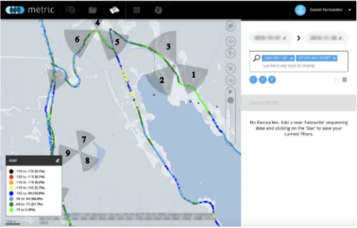
FIGURE 1. Scenario A depicted in Metric platform.
The first scenario has 9 transmitting antennas, numbered and identified in Fig.1, and the second scenario has only 1 transmitting antenna. All the antennas have a transmission power, Ptx, of 46 dBm, they work at a downlink frequency
of 796 MHz, and are located in an urban area. For each of the antennas, the respective horizontal and vertical radiation pattern was considered, and the gain of the receiver antenna (in downlink scenario the MT antennas) is 0 dB. More details of the antennas parameters are presented in Table1.
TABLE 1.Synthesis of antennas parameters.
The selected DTs for both scenarios were collected by the operator within a time-window of 2 months, and then loaded into the Metric platform where they were dumped and processed in a transparent way. We required DTs with this time interval to ensure that the antenna parameters
were not changed in between, to ensure that the overall network configuration remained unchanged for this study. This interval is then divided into two sets in order to allow the calibration of the models and subsequently the assessment of the estimation accuracy. These two sets are divided temporally, being the first identified by period t, and the second, t + 1. The terminology t and t + 1 is considered in order to allow the understanding of temporal continuity. This means the evaluation of the estimation (period t + 1) is carried out sequentially after the considered calibration period (period t).
The first scenario, scenario A, has 9 transmitting antennas, which presents a total of 2791 DTs in period t for the calibration of the ACSPM and 1126 DTs in period t + 1 for evaluation of both models (ACSPM and AIPM). This scenario is depicted in Fig.1.
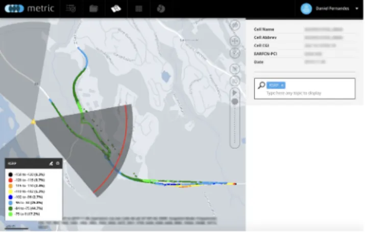
In scenario B, presented in Fig.2, the antenna is located approximately 22 km away from the antennas in scenario A, thus maintaining the same population density and buildings topology. This scenario is divided into 2 sub-scenarios in order to evaluate the impact on the ACSPM accuracy when the number of DTs used in its calibration changes. In sub-scenario B.1, 698 DTs are used in the calibration of the ACSPM and 1033 in the evaluation of both models (ACSPM and AIPM). In sub-scenario B.2 the number of DTs used to calibrate the ACSPM model increases to 1270. For evaluating the accuracy, 40 DTs were needed.
FIGURE 2. Scenario B depicted in the Metric platform.
A summary of the DTs number in each time interval for each scenario is detailed in Table2.
TABLE 2. Specification of the number of DTs for each scenario, for the calibration (t ) and evaluation (t + 1) time periods.
C. PERFORMANCE EVALUATION METRICS
To compare the results achieved by different propagation models, some metrics of statistical analysis were chosen to analyse the results in several aspects.
These metrics will compare real values, Prx, and the
esti-mated values, ˆPrx, for each model. N represents the number of samples considered in the comparison. Each of the metrics chosen is now detailed:
• Mean Absolute Error (MAE): The MAE measures the
average absolute error between the real data and the estimated data. MAE is one of the most common metrics to evaluate the performance of regression models. The expression used in the MAE calculation is given by the following equation (2) [18]. MAE[dB] = 1 N · N X i=1 |Prxi − ˆPrxi|. (2)
When MAE values are close to 0, the estimated data nearly matches the real data.
• Standard Deviation (σ): The standard deviation
mea-sures the dispersion of values in relation to a mean value. When the estimated values are close to its mean values the standard deviation value tends to 0. The value of the standard deviation can be given by (3) [19].
σ [dB] = s
PN
i=1(Prxi − Prx)2
N −1 , (3)
where Prxdenotes the average value of Prx.
• Pearson Correlation Coefficient (r): The correlation
coefficient measures the degree of relationship between real and estimated measures. This coefficient can vary between -1 and 1 depending on whether it is a positive or negative correlation. This coefficient is calculated using equation (4) [20]–[22]. r = PN i=1(Prxi− Prx) · PN i=1( ˆPrxi− ˆPrx) q PN i=1(Prxi− Prx)2· q PN i=1( ˆPrxi − ˆPrx)2 , (4) where Prxand ˆPrx denotes the average value of Prx and
ˆ
Prx respectively.
Depending on the calculated absolute value of r the relationship between the measurements can be classified according to Table3[21].
TABLE 3.Correlation classification.
According to [13], a propagation model is considered accurate when MAE is nearly 0, theσ is less than 9 dB and the coefficient of correlation, |r|, is more than 0.8.
III. COVERAGE ESTIMATION METHODOLOGIES
Coverage in cellular networks is essential. Its estimation can be done following different methodologies. The ACSPM is
suited for operating cells with DT, KPI and CM data of their operation. On the other hand, AIPM is suited for estimating the received signal close to new antenna locations, using available DT information from neighboring operating cells. These two models are detailed next.
A. SEMI-EMPIRICAL PROPAGATION MODEL
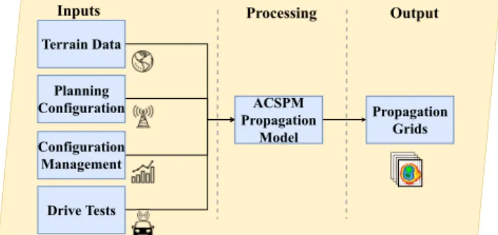
The proposal for a new cloud-based framework of a semi-empirical propagation model is presented and detailed in [7]. This propagation model, called ACSPM has as main innovation the automatic model calibration and estimation of a received signal area using DTs reporting its signal within its service area, as well as CM and KPI data related to its operation. The cell coverage estimation model is represented in Fig.3.
FIGURE 3. Cell coverage estimation model framework.
As indicated in Fig. 3the inputs of the signal estimation framework are the data of terrain altimetry, the network configuration such as antenna location, or its operating parameters. The operator uses KPIs and DTs to make a fine-tuning and adjustment of the propagation model with the reality in order to portray a more realist approach of the network.
At the processing level, this semi-empiric model is based on two well-known propagation models, which are Walfish-Ikegami [23] and SPM [3]. The ACSPM combines these two models in order to build a new propagation model that can be used both in micro and macro cells.
The result of this propagation model is the creation of a grid with the signal received around an antenna that enables operators to perform various planning and network optimisation tasks.
As previously mentioned, one of ACSPM’s innovations is the automatic calibration and generation of propagation grids. This propagation model, implemented using cloud services, was integrated into Metric platform. When new network information for a given antenna is available, such as DTs, KPI or configurations, the model is automatically calibrated and a new propagation grid is generated for that antenna allowing the operator to have a current status of the network. This automation follows the SON paradigm, as allows the implementation of this framework in SON systems since it allows the reduction of human actions in the network
because if there is a problem of network coverage it can be immediately detected through the automatically updated propagation grids, and then trigger the actions necessary to solve it. Since this processing is very intensive and uses a lot of computational resources, Metric transfers its computation to micro cloud services, namely the services provided by Amazon Web Services (AWS) [24].
B. MACHINE LEARNING PROPAGATION MODEL
Artificial Intelligence (AI) is a recurrent term nowadays and its main objective consists in solving specific problems by executing specific tasks. It is embedded in techniques and tools that execute those tasks. By being a difficult challenge for humans to perform and execute these tasks intuitively, for machines it is only a very challenging set of applied algorithms.
Artificial Neural Networks (ANNs) refers to artificial networks of neurons that were inspired (and they are very similar) to the natural functioning of a human brain [25]. Neurons, both natural and artificial ones, are the fundamental units responsible by the computation process. They are interconnected to form a network of data processing. Each individual neural has inputs and outputs and they are responsible to ‘‘consume’’ the data from the input in order to generate an output. These outputs, in the natural brain, can be, for example, responses to human reactions like emotions or sensations. The same outputs in an artificial neuron are expected to achieve a desired output. A common neural network is divided in three layers: the input layer, the hidden layers and the output layer. These layers are responsible for the input data (input layer), the intermediary layers that process the data, and the output layer that generates a result. Fig.4depicts an example of an ANN’s architecture design.
FIGURE 4. Configuration example of an ANN with three neurons in the input layer, one hidden layer and two output neurons.
The ANNs are much less complex that the natural ones, but both share a common principle: There is a ‘‘learning’’ process that is achieved when neurons reconnect each other. They can learn by ‘‘looking’’ at the input data - input dataset - and with that, they recognise patterns or structures within that data (learning or training process). A training dataset is composed by a set of input data and a set of output data, in which the ANN will try to estimate the output by learning the data characteristics and properties in
order to achieve the desired output given by the output data (supervised learning). This knowledge is then applied on other datasets in order to estimate, classify or predict the same (or a similar) results on unknown data (generalisation or validation process). However, there is always a difference between the estimated value given by the ANN and the real outputs values. This difference is called ‘‘error’’ or ‘‘loss’’ and is the value responsible to evaluate the ANN model’s performance [26], [27].
AI-based algorithms are known to be capable to process great amounts of data. When AI is applied to the telecommu-nications area, there are some tasks that require great amounts of data too. In this article, an AI-generated model will be used to predict path loss. [28] and [29] also used AI algorithms to estimate path loss regression for a given area.
In order to develop and implement the AI algorithm for this investigation, a custom ANN must be designed. The chosen ANN architecture is formed by 3 neurons in the input layer, 2 hidden layers with 5 and 3 neurons, respectively, and 1 neuron in the output.
As identified in Fig. 5, the input dataset contains, for each point, geographical information (latitude, longitude, and height), the distance from that location to the BS, the antenna gain at that same location and, finally, the losses that occur between transmission and reception. The output is the path loss value to reach that position. After testing several architectures that implement the ANN algorithm, the architecture depicted in Fig.5was the one presenting the best results, therefore it was chosen for further calibration and training.
FIGURE 5. Custom architecture design of the implemented ANN algorithm.
C. PROPAGATION MODELS TUNING/CALIBRATION
To apply the propagation models to the different scenarios presented, it is necessary to fine-tune them. For the ACSPM, its calibration occurs in each antenna, and is not applicable to others. According to [7], in DT locations there is no error between ACSPM and the DT measures (since the model uses the DT values whenever possible); for neighboring pixels, the values are calculated by weighting neighboring DTs, using all inputs as depicted in Fig.3. In terms of accuracy, this model can achieve a MAE of about 5 dB.
The AIPM is a different model. Once calibrated/generated with available DT measurements from multiple antennas, the AIPM can generate coverage grids for any antenna location in the scenario area.
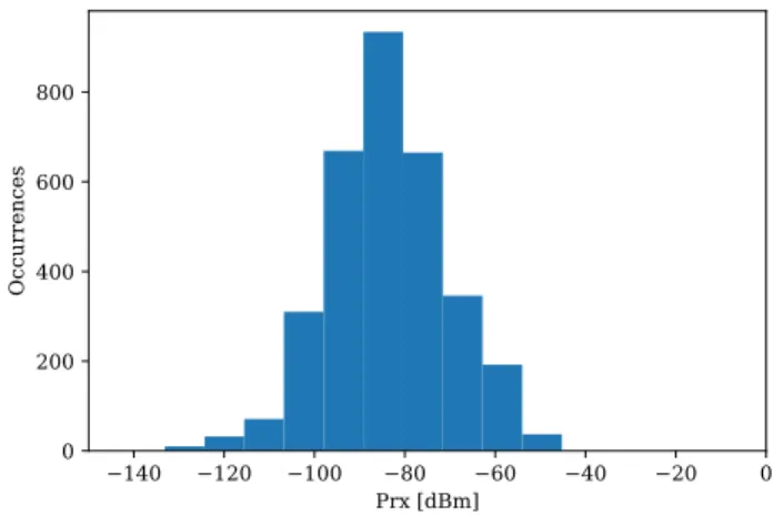
To better characterise the Reference Scenarios presented in SectionII-B, the AIPM was generated with 13740 DTs as input data, collected from 31 antennas located in an urban environment, in the same geographical area in time period t. These 31 antennas include the antennas of scenarios A and B. The DTs of the input data present a mean value of −83.6 dBm and a standard deviation of 13.1 dBm. The histogram with the distribution of the DT values is depicted in Fig.6and it is possible to see that the achieved mode for the received power level, Prx, of each DT lies between −70 dBm and −98 dBm.
FIGURE 6. DT occurrences distributed by their Prxvalue.
For the AIPM configuration, it was considered a dataset of DTs from period t, being 80% used for the training process and 20% for the validation process. To achieve the best possible performance, the chosen network configuration was trained along 1000 iterations, and by using callbacks, only the model that reached the lowest MAE value was stored. Since training is a random process, the chosen network configuration was trained 20 times and only the training with the lowest MAE value was considered.
The training that reached the best MAE values, which was 8.6 dB, took 16 seconds to train. In Fig.7, the evolution of training and validation curves is depicted. Once the model has been trained, it can be applied to any scenario by simply predicting the data inputs provided. For scenario A, the prediction was done in 15 seconds, when using the AIPM model. For the case of ACSPM, the model had to be calibrated for each scenario, which resulted in about 173 seconds, for combining the results for scenario A and the estimation for each of the 9 antennas.
By analysing Fig. 7, it is possible to conclude that the training process converged smoothly and the loss values were very stable during the whole process, reaching its optimal values very quickly. It is also possible to conclude that the model achieved an acceptable performance. In order to
FIGURE 7. Loss values of Training and Validation sets.
develop the AI-generated model, a frontend framework called
Keras[30] was used, which uses TensorFlow [31] as backend. IV. RESULTS COMPARISON
In this section, the results for the metrics presented in SectionII-Care discussed for each of the scenarios presented
in Section II-B when the AIPM and ACSPM models
presented in SectionIIIare applied.
A. SCENARIO A
This scenario has 2791 DTs in time period t which are used to calibrate the ACSPM model. In period t + 1, 1126 DTs are used for performance evaluation purposes. For each of those models, a received signal power grid was obtained. In Fig. 8the grid for the AIPM is shown and in Fig.9 the result estimated with the ACSPM model. The ACSPM model initially estimates the coverage area for each of the antennas in the scenario and then all the areas are overlapped in a single area.
FIGURE 8. Estimated received power level using the AIPM model for the entire service area and considering all the antennas for scenario A.
By analysing the shapes, which are similar in each generated model, it is noticeable that ACSPM is a more optimistic model, since the green area (where Prx lies
FIGURE 9.Estimated received power level using the ACSPM model for the entire service area and considering all the antennas for scenario A.
between 0 dBm and −75 dBm) is greater. The results estimated by these models were compared with the real values. The AIPM obtained a MAE of 7.1 dB, which is 0.1 dB lower than the ACSPM. When comparing theσ of the AIPM with that of ACSPM, the AIPM obtains values which are 2.4 dB lower. r is 0.73 for the AIPM and 0.58 for the ACSPM. For this scenario, according to the considered metrics, AIPM achieves better performance results when compared with ACSPM.
It can be concluded that, for the estimation of coverage within a scenario of several cells, AIPM achieves good and useful results. It is not needed to build individual grids of realistic coverage estimations for each antenna and to combine them.
B. SCENARIO B.1
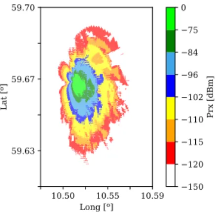
In this single antenna scenario, depicted in Fig.10, unlike the multi-antenna scenario, the ACSPM is the model that presents an area where the signal coverage between 0 dBm and −96 dBm is lower. For the same propagation area, the AIPM shape, depicted in Fig.11, is much more extended when compared to the shape estimated by the ACSPM.
FIGURE 10. Estimated received power level using the ACSPM model for scenario B.1.
In this analysis with the chosen metrics, the ACSPM presents a MAE of 7.3 dB while the AIPM presents 7.2 dB.
FIGURE 11. Estimated received power level using the AIPM model for scenario B.1.
For the case of σ , the AIPM is 3 dB better. However, the ACSPM presents a value of 0.73 for r, which is higher than that obtained with AIPM, which is 0.69. Therefore, in terms of, r, the ACSPM model is slightly better, since it presents a greater correlation between estimated and real data. This is due to the fact that here we are using a single antenna, which requires a more realistic estimation of coverage based on standard propagation aspects, and AIPM does not take it into account.
C. SCENARIO B.2
For scenario B.2, the received signal grid estimated by ACSPM is presented in Fig.12. For the AIPM the estimation is the same as in B.1 scenario, as shown in Fig.11.
As noticed in scenario B.1, the AIPM presented better results. To try to improve the results of the ACSPM for the same scenario, the number of DTs used in the calibration of the ACSPM was increased. This increase improved all metrics. The ACSPM presents a MAE of 6.6 dB with a variation of 4.1 dB. In this scenario, the correlation between the measurements can be classified as ‘‘very strong’’ since the value of r obtained is 0.82. For the AIPM the MAE decreased to 6.0 dB with a variation of 4.0 dB. The correlation has a value of 0.80.
D. SUMMARY
The fact that B scenarios addresses the estimation of coverage of a single antenna, while A scenario addresses the best signal level for a set of antennas, naturally affects the results. Nevertheless, each of the approaches is needed and has useful applications in the study and evaluation of a network.
Scenarios A and B show that the estimated grids for the signal level received have similar shapes for each of the models, the values of MAE differ, at most 0.5 dB from each other, which indicates that the models have similar performance.
Table4presents a summary with the values achieved for each metric and for each scenario.
FIGURE 12. Estimated received power level using the ACSPM model for scenario B.2.
TABLE 4.Synthesis of results for each of the scenarios understudy.
By analysing Table 4, we observe that both models achieved similar MAE values. It is also verified that, as the number of DTs used in the model performance evaluation decreases, the value of the MAE also decreases, as presented in scenario B.2. The ACSPM model presents the highest variation between the samples tested, indicating a higher error associated with the signal level estimation. In scenarios B.1 and B.2, both models present a similar relationship between estimated and real measures. This situation changes in scenario A where the AIPM has a higher relationship of 0.15 when compared to the ACSPM.
Following the conditions presented at the end of SectionII-C, both ACSPM and the AIPM can be considered as an accurate propagation model for B.2 scenario, for estimation of coverage of a single antenna, since in the remaining scenarios all models have a value of r less than 0.80. In fact, it is understandable that AIPM needs large data sets to provide realistic results, as a semi-empirical propagation model integrates physical aspects that are realistic (e.g., power decay with distance).
These results also indicate that, by increasing the number of DTs used in the ACSPM calibration, the signal estimation for that antenna improves. If we increase the number of DTs for the AIPM training, the model becomes more robust for estimating coverage of new antennas, as we should expect. V. CONCLUSION
Cellular network operators collect large amounts of DTs, measuring the signal strength received by antennas geolo-cated along a given path. These can be very useful to estimate
coverage for operating cells using the ACSPM model and for new cells, using the AIPM. Since AI can solve several problems in a simple, fast, and effective way and its solutions can be quite optimised, this study focused on comparing the performance of ACSPM, a semi-empirical propagation model with realistic results, with that of a model generated by AI.
The results achieved demonstrate that the ACSPM, which was designed for only one antenna at a time, obtains quite homogeneous results for that scenario or even when the estimation of each of the antennas is combined in a multi-antenna scenario to estimate the overall coverage of the network. It reaches an average MAE of 7.0 dB decreasing when the number of DT used in the calibration of the model is increased.
The AIPM presents similar results to the ACSPM, however, it can still overcome the results of this model by 0.5 dB. The use of these models is quite interesting because it does not require any previous knowledge of the propagation models.
As demonstrated the number of DTs used in the calibration of ACSPM or in the training of AIPM has a powerful impact on results, so, the greater the number of DTs the better the results achieved. By using a wide range of DTs for the training of the AIPM model, we can also use it in regions that are geographically similar.
The research and results undertaken with these models made it possible to foresee new applications for them. Since both exhibit quite similar performances, the ACSPM can be applied to estimate the coverage of existing cells using DTs, while the AIPM, once trained, useful for the deployment of new cells, in the same geographical area, based on the first estimation.
In terms of computational efficiency, AIPM is a model that presents results very quickly, while ACSPM requires more time, as it presents a greater computational complexity, and it can output much more detailed results.
As we have verified, the performance results achieved can be greatly improved by increasing the number of DTs. This increase in the number of DTs, which can be achieved by using MDTs, allows a much more efficient and precise training/calibration of the models, allowing to accurately portraying a region for a more accurate network planning and coverage.
The research results presented in this article are based on a Single Input Single Output (SISO) communication system. However with the evolution to 5G technology where, Multiple Input Multiple Output (MIMO) systems are used, it can be interesting to know the effective impact on the propagation of the signals by applying these models to a MIMO system.
REFERENCES
[1] Ericsson Mobility Report 2019, Ericsson, Stockholm, Sweden, Nov. 2019. [2] W. C. Hardy, QoS—Measurement and Evaluation of Telecommunications
Quality of Service. Hoboken, NJ, USA: Wiley, Jul. 2001.
[3] Atoll 3.3.0 Technical Reference Guide for Radio Networks, Forsk, 2015. [4] Metric. Accessed: Apr. 1, 2020. [Online]. Available: https://metric.pt
[5] Multivision. Accessed: Apr. 1, 2020. [Online]. Available: https:// multivision.pt
[6] OptiNET-5G—Planning and Optimization Framework of 5G
Heteroge-neous Networks in a Cloud Environment, Multivision, Eur. Union, Funded Centro, Portugal, 2020.
[7] D. Fernandes, D. Clemente, G. Soares, P. Sebastiao, F. Cercas, R. Dinis, and L. S. Ferreira, ‘‘Cloud-based implementation of an automatic coverage estimation methodology for self-organising network,’’ IEEE Access, vol. 8, pp. 66456–66474, 2020.
[8] M. Frankel, N. Shacham, and J. E. Mathis, ‘‘Self-organizing networks,’’
Future Gener. Comput. Syst., vol. 4, no. 2, pp. 95–115, Sep. 1988. [9] K. Zheng, Z. Yang, K. Zhang, P. Chatzimisios, K. Yang, and W. Xiang,
‘‘Big data-driven optimization for mobile networks toward 5G,’’ IEEE
Netw., vol. 30, no. 1, pp. 44–51, Jan. 2016.
[10] I. Popescu, I. Nafornita, G. Gavriloaia, P. Constantinou, and C. Gordan, ‘‘Field strength prediction in indoor environment with a neural model,’’ in
Proc. 5th Int. Conf. Telecommun. Mod. Satell., Cable Broadcast. Service, 2001, pp. 640–643.
[11] E. Ostlin, H. Zepernick, and H. Suzuki, ‘‘Macrocell path-loss prediction using artificial neural networks,’’ IEEE Trans. Veh. Technol., vol. 59, no. 6, pp. 2735–2747, Jul. 2010.
[12] J. M. Mom, C. O. Mgbe, and G. A. Igwue, ‘‘Application of artificial neural network for path loss prediction in urban macrocellular environment,’’
Amer. J. Eng. Res., vol. 3, no. 2, pp. 270–275, 2014.
[13] M. Ayadi, A. B. Zineb, and S. Tabbane, ‘‘A UHF path loss model using learning machine for heterogeneous networks,’’ IEEE Trans. Antennas
Propag., vol. 65, no. 7, pp. 3675–3683, Jul. 2017.
[14] A. F. Molish, Wireless Communications, 2nd ed. Hoboken, NJ, USA: Wiley, 2010.
[15] M. F. Iskander and Z. Yun, ‘‘Propagation prediction models for wireless communication systems,’’ IEEE Trans. Microw. Theory Techn., vol. 50, no. 3, pp. 662–673, Mar. 2002.
[16] F. Letourneux, S. Guivarch, and Y. Lostanlen, ‘‘Propagation models for heterogeneous networks,’’ in Proc. 7th Eur. Conf. Antennas Propag.
(EuCAP), 2013, pp. 3993–3997.
[17] W. A. Hapsari, A. Umesh, M. Iwamura, M. Tomala, B. Gyula, and B. Sebire, ‘‘Minimization of drive tests solution in 3GPP,’’ IEEE Commun.
Mag., vol. 50, no. 6, pp. 28–36, Jun. 2012.
[18] C. Willmott and K. Matsuura, ‘‘Advantages of the mean absolute error (MAE) over the root mean square error (RMSE) in assessing average model performance,’’ Climate Res., vol. 30, no. 1, pp. 79–82, 2005. [19] P. Barde and M. Barde, ‘‘What to use to express the variability of data:
Standard deviation or standard error of mean?’’ Perspect. Clin. Res., vol. 3, no. 3, pp. 113–116, 2012.
[20] E. Östlin, H. Suzuki, and H.-J. Zepernick, ‘‘Evaluation of the propagation model recommendation ITU-R P.1546 for mobile services in Rural Australia,’’ IEEE Trans. Veh. Technol., vol. 57, no. 1, pp. 38–51, Jan. 2008.
[21] M. J. Campbell and T. D. V. Swinscow, Statistics at Square One, 11th ed. Hoboken, NJ, USA: Wiley, 2011.
[22] H. Wang, W. Du, and X. Chen, ‘‘Evaluation of radio over sea propagation based ITU-R recommendation P.1546-5,’’ J. Commun., vol. 10, no. 4, pp. 231–237, 2015.
[23] A. R. Mishra, Ed., Advanced Cellular Network Planning and Optimisation. Chichester, U.K.: Wiley, Oct. 2006.
[24] AWS. Accessed: Apr. 1, 2020. [Online]. Available: https://aws.amazon.com [25] L. Wang, O. Kisi, M. Zounemat-Kermani, G. A. Salazar, Z. Zhu, and W. Gong, ‘‘Solar radiation prediction using different techniques: Model evaluation and comparison,’’ Renew. Sustain. Energy Rev., vol. 61, pp. 384–397, Aug. 2016.
[26] A.I. Wiki. Accessed: Apr. 15, 2020. [Online]. Available: https://pathmind. com/wiki/neural-network
[27] P. M. Buscema, G. Massini, M. Breda, W. A. Lodwick, F. Newman, and M. Asadi-Zeydabadi, ‘‘Artificial neural networks,’’ Stud. Syst., Decis.
Control, vol. 131, pp. 11–35, 2018.
[28] S. I. Popoola, E. Adetiba, A. A. Atayero, N. Faruk, and C. T. Calafate, ‘‘Optimal model for path loss predictions using feed-forward neural networks,’’ Cogent Eng., vol. 5, no. 1, 2018, Art. no. 1444345.
[29] Y. Zhang, J. Wen, G. Yang, Z. He, and J. Wang, ‘‘Path loss prediction based on machine learning: Principle, method, and data expansion,’’ Appl. Sci., vol. 9, no. 9, p. 1908, May 2019.
[30] Keras. Accessed: Apr. 15, 2020. [Online]. Available: https://keras.io/ [31] TensorFlow. Accessed: Apr. 15, 2020. [Online]. Available:
DANIEL F. S. FERNANDES received the B.S. degree in telecommunications and computer engi-neering and the M.S. degree in telecommunica-tions and computer engineering from ISCTE-IUL, Lisbon, Portugal, in 2012 and 2017, respectively, where he is currently pursuing the Ph.D. degree in information science and technology. As a Researcher, he is currently working at Multivision, Consultoria Informática. His research interests include telecommunications and 5G networks. He has six scientific publications as the author in journals or at international conferences and nine scientific publications as a coauthor.
ANTÓNIO RAIMUNDO received the B.Sc. degree in computer science and the M.Sc. degree in computer science from the ISCTE-Lisbon University Institute, Lisbon, Portugal, in 2014 and 2016, respectively, where he is currently pursuing the Ph.D. degree in information science and technology. Since 2016, he has been a Junior Researcher with the Instituto de Telecomuni-cações, ISCTE-IUL branch, Lisbon. His research interest includes the development of applications for Unmanned Aerial Vehicles (UAVs), using machine learning techniques. His Ph.D. research topics explore computer vision methods to perform automated classification by using UAVs on industrial applications.
FRANCISCO CERCAS (Senior Member, IEEE) received the Ph.D. degree from Lisbon University, Portugal, in 1996. He was a Researcher with INESC, from 1984 to 1985, CAPS, from 1986 to 1993, and the Instituto de Telecomunicações, in 1994. He was also a Visiting Researcher with the University of Plymouth, U.K., from 1987 to 1992. He is currently a Full Professor with more than 36 years of professional experience including Research and Development at the industry and 35 years of university teaching at the Instituto Superior Técnico, Lisbon University, and ISCTE–University Institute of Lisbon, in 1999. He has participated in more than a dozen European Projects in the telecommu-nications area, namely as the Portuguese Delegate in four COST actions (European Cooperation in Science and Technology). He is the author and/or coauthor of a new class of codes, Tomlinson, Cercas, Hughes (TCH), one patent, and about 200 publications including book chapters, journal articles, and conference papers. He also supervised many Ph.D.’s and M.Sc.’s. His research interests include satellite and mobile communications, coding theory, spread spectrum communications, and related topics.
PEDRO J. A. SEBASTIÃO (Member, IEEE) received the Ph.D. degree in electrical and com-puter engineering from IST. He is currently a Professor with the ISCTE–IUL’s Information Sci-ence and Technology Department. He is the Board Director of the AUDAX-ISCTE-Entrepreneurship and Innovation Center, ISCTE, responsible for the LABS LISBOA incubator and a Researcher at the Institute of Telecommunications. He has oriented several master’s dissertations and Ph.D. theses.
He is the author or coauthor of more than two hundred scientific articles and he has been responsible for several national and international Research and Development projects. He has been an Expert and Evaluator of more than one hundred national and international Civil and Defense Research and Development projects. It has several scientific, engineering, and pedagogical awards. Also, he has organized or co-organized more than fifty national and international scientific conferences. He planned and developed several postgraduate courses in technologies and management, entrepreneurship and innovation, and transfer of technology and innovation. He has supported several projects involving technology transfer and creation of start-ups and spin offs of value to society and market. He has developed his professional activity in the National Defense Industries, initially in the Office of Studies and later as the Board Director of the Quality Department of the Production of New Products and Technologies. He was also responsible for systems of communications technology in the Nokia-Siemens business area. His main research interests include monitoring, control and communications of drones, unnamed vehicles, planning tools, stochastic process (modeling and efficient simulations), the Internet of Things, and efficient communication systems.
RUI DINIS (Senior Member, IEEE) received the Ph.D. degree from the Instituto Superior Técnico (IST), Technical University of Lisbon, Portugal, in 2001, and the Habilitation degree in telecommunications from the Faculdade de Ciências e Tecnologia (FCT), Universidade Nova de Lisboa (UNL), in 2010. From 2001 to 2008, he was a Professor with IST. He is currently an Associated Professor with FCT-UNL. In 2003, he was an Invited Professor with Carleton Univer-sity, Ottawa, Canada. He was a Researcher with the Centro de Análise e Processamento de Sinal (CAPS), IST, from 1992 to 2005, and a Researcher with the Instituto de Sistemas e Robótica (ISR), from 2005 to 2008. Since 2009, he has been a Researcher with the Instituto de Telecomunicações (IT). He has been actively involved in several national and international research projects in the broadband wireless communications area. His research interests include transmission, estimation, and detection techniques. He is a VTS Distinguished Lecturer and is or was Editor at the IEEE TRANSACTIONS ONWIRELESSCOMMUNICATIONS, the IEEE TRANSACTIONS ONCOMMUNICATIONS,
the IEEE TRANSACTIONS ONVEHICULARTECHNOLOGY, the IEEE OPENJOURNAL ONCOMMUNICATIONS, and Physical Communication (Elsevier). He was also a Guest Editor for Physical Communication (Elsevier), special issue on broadband single-carrier transmission techniques.
LÚCIO S. FERREIRA (Senior Member, IEEE) received the Licenciado (five years) and Ph.D. degrees in electrical and computer engineering from the IST, Technical University of Lisbon, Portugal. As a Researcher, he worked Deutsche Telekom Innovation Laboratories in 1998, Insti-tuto de Telecomunicações, from 1999 to 2012, INOV-INESC, from 2012 to 2015. He has been a Researcher with INESC-ID, since 2016. As an Assistant Professor, he has worked with the Uni-versidade da Beira Interior, the UniUni-versidade Lusiada de Lisboa, and ISTEC, in the areas of computer science and telecommunications. He is currently also a Project Manager with the Multivision, Consultoria Informatica. He participated, as a Project Manager and a Researcher, in 17 Research and Development projects funded by the European Commission, At national level, he has worked as a Consultant for mobile providers and ANACOM national regulator. He has more than 50 scientific publications in books, journal articles, and international conferences. He is the Editor and a co-author of 63 technical reports for the European Commission. He reviewed 29 journal articles and conference papers, and participated in eight organizational committees and 15 technical committees of international conferences. He has supervised 12 M.Sc. and three Ph.D. students. He is a Board Member of the IEEE ComSoc Portugal Chapter.