energies
ArticleA Comparison of Energy Consumption Prediction
Models Based on Neural Networks of
a Bioclimatic Building
Hamid R. Khosravani1,2, María Del Mar Castilla3,*, Manuel Berenguel3, Antonio E. Ruano1,2 and Pedro M. Ferreira4
Received: 15 October 2015; Accepted: 12 January 2016; Published: 20 January 2016 Academic Editor: Chi-Ming Lai
1 Faculty of Science and Technology, University of Algarve, Campus Gambelas, Faro, Portugal;
[email protected] (H.R.K.); [email protected] (A.E.R.)
2 Institute of Mechanical Engineering (IDMEC), Instituto Superior Técnico, Universidade de Lisboa,
Lisboa, Portugal
3 Department of Computer Science, Automatic Control, Robotics and Mechatronics Research Group,
University of Almería, Agrifood Campus of International Excellence (ceiA3), CIESOL, Joint Center University of Almería-CIEMAT, Almería, Spain; [email protected]
4 LaSIGE, Faculdade de Ciências, Universidade de Lisboa, Portugal; [email protected] * Correspondence: [email protected]; Tel.: +34-950-21-41-55; Fax: +34-950-01-51-29
Abstract:Energy consumption has been increasing steadily due to globalization and industrialization. Studies have shown that buildings are responsible for the biggest proportion of energy consumption; for example in European Union countries, energy consumption in buildings represents around 40% of the total energy consumption. In order to control energy consumption in buildings, different policies have been proposed, from utilizing bioclimatic architectures to the use of predictive models within control approaches. There are mainly three groups of predictive models including engineering, statistical and artificial intelligence models. Nowadays, artificial intelligence models such as neural networks and support vector machines have also been proposed because of their high potential capabilities of performing accurate nonlinear mappings between inputs and outputs in real environments which are not free of noise. The main objective of this paper is to compare a neural network model which was designed utilizing statistical and analytical methods, with a group of neural network models designed benefiting from a multi objective genetic algorithm. Moreover, the neural network models were compared to a naïve autoregressive baseline model. The models are intended to predict electric power demand at the Solar Energy Research Center (Centro de Investigación en Energía SOLar or CIESOL in Spanish) bioclimatic building located at the University of Almeria, Spain. Experimental results show that the models obtained from the multi objective genetic algorithm (MOGA) perform comparably to the model obtained through a statistical and analytical approach, but they use only 0.8% of data samples and have lower model complexity.
Keywords: predictive model; electric power demand; neural networks; multi objective genetic algorithm (MOGA); data selection
1. Introduction
Due to fast economic development affected by industrialization and globalization, energy consumption has been steadily increasing over the last years [1,2]. Industry, transportation and buildings are the three main economic sectors which consume a significant amount of energy, with buildings accounting for the biggest proportion. For example in European Union countries, energy consumption in buildings represents about 40% of the total energy consumption [3]. In the
Energies 2016, 9, 57 2 of 24
USA, more than 44% of domestic energy consumption corresponds to heating, ventilating and air conditioning (HVAC) systems in buildings [4]. Studies have shown that by following the current energy consumption pattern, the world energy consumption may increase more than 50% before 2030 [5], while most of the energy resources are not renewable in nature. Moreover, the usage of energy causes environmental degradation [2]. Therefore, energy consumption management is a very significant problem not only to tackle the losses resulting from increasing consumption patterns but also to improve the performance of building energy systems. With respect to energy management, a variety of policies have been considered. In recent years, there has been a focus on bioclimatic architectures for buildings to reduce the indoor consumption of energy. In this kind of architecture, buildings are designed based on the local climate conditions. These include wind speed and direction, daily exterior temperature and relative humidity, as well as diverse passive solar technologies where heating and cooling techniques passively absorb solar radiation or protect from it without containing mobile elements [6–8]. Besides environmental variables, physical properties of buildings are considered in bioclimatic architectures, such as shape, buildings’ orientation related to the sun and wind, wall thickness and roof construction [6,9].
Utilizing renewable energy sources such as biomass, hydropower, geothermal, solar, wind and marine energies have been considered as alternatives for conventional energy resources in most developed and developing countries [10,11]. In the European Union, the renewable energies use share is 20% of the total energy consumption and 10% of renewable energies will be used in transportation by 2020 [12]. Using renewable energies not only helps ensure the security of non-renewable energy supply in future, but also minimizes environmental degradation [11].
Prediction of energy use in buildings has received a remarkable amount of attention from researchers [1,3,13,14], as an approach to reduce energy consumption, which is intended to conserve energy and reduce environmental impacts [3]. The prediction of energy usage in buildings and modelling the behaviour of the corresponding energy system, are complicated tasks due to influential factors such as weather variables, building construction, thermal properties of the physical materials and occupants’ activities [3]. Furthermore, there are several nonlinear inter-relationships among the involved variables, often in a noisy environment, which amplify the difficulty in identifying the precise interaction among them [15].
The methods aiming to predict building energy consumption can be categorized mainly into statistical, engineering and artificial intelligence ones. A review on prediction methods can be found in [3,16]. Engineering methods, which are detailed comprehensive methods, use the structural properties of buildings in the form of physical principles and thermal dynamics equations, as well as environmental information such as climate conditions, occupants, their activities and HVAC equipment parameters. On the one hand, these methods need a high level of details about the structural and thermal parameters of buildings that are not always available and, on the other hand, since engineering methods depend on complex physical principles, a high level of expertise is needed to elaborately develop the corresponding models [3,17]. To reduce the complexity of the detailed comprehensive engineering methods, simplified methods have been proposed, which can be seen in [18,19].
Statistical methods use historical data to correlate energy consumption as target with most influential variables as inputs. Hence, the quality and quantity of historical data has a crucial role in developing statistical models [17,20]. Unlike engineering methods, statistical methods provide models with a smaller number of variables and much less physical understanding. Regression models, conditional demand analysis (CDA), auto regressive moving average (ARMA), auto regressive integrated moving average (ARIMA) and Gaussian mixture models (GMM) are some instances of statistical models [20–23].
In recent years, artificial intelligence methods such as neural networks, support vector machines and fuzzy logic have been widely considered in applications of energy consumption. Like statistical methods, artificial intelligence methods use historical data reflecting the behaviour of the process to be modelled. Neural networks have shown a high capability to capture complex nonlinear relationships
Energies 2016, 9, 57 3 of 24
between inputs and outputs. Since the energy consumption process has a nonlinear behaviour, neural networks are mostly applied in this domain. In addition, they are quicker and easier to develop than engineering and statistical methods, while being accurate estimators. Some instances of neural network based models may be found in [15,17,24–28].
Recently, support vector machines have received much attention as quick methods to build predictive models in energy consumption applications. They can provide models with a high level of generalization based on a number of data. Applications to the prediction of energy utilization can be viewed, for instance, in [29–31].
Besides neural network- and support vector machine-based models, another kinds of models which benefit from fuzzy logic have been considered. Fuzzy logic deals with imprecise reality and handles the concept of truth value ranging between completely true and completely false (1–0) [32]. Some models of this type can be seen in [33,34].
As mentioned earlier, both statistical and artificial intelligence methods need sufficient historical data to provide accurate models. In cases where limited amounts of data are available and the information about the process to be modelled is partially known, grey models are suitable alternatives to the prediction of time series associated with processes [35–37].
The objective of this paper is to compare a neural network based model obtained in [17] with the models obtained by a multi objective genetic algorithm (MOGA), to predict the electric power demand of the Solar Energy Research Center (Centro de Investigación en Energía SOLar or CIESOL in Spanish) building located at University of Almeria, Spain. The authors in [17] determined the structure and the order of the model by statistical and analytical methods while in this article a non-dominated set of models is generated by a MOGA considering a set of objectives to be optimized. For the sake of completion, the performance of MOGA models is also compared with the results obtained by a naive autoregressive baseline (NAB) approach, introduced in [38].
This paper is organized as follows: in Section2, the structural properties and power demand profile of the CIESOL building are briefly described. The model proposed in [17] and the models generated by MOGA are widely described in Sections3and4respectively. Experimental results are shown in Section5. Finally, some conclusions are drawn in Section6.
2. Experimental Setup: The Solar Energy Research Center Building
The CIESOL building (Figure1a), is a mixed solar energy research centre operated between the Centre for Energy, Environment and Technology (in Spanish the Centro de Investigaciones Energéticas, MedioAmbientales y Tecnológicas—CIEMAT) and the University of Almería, situated in the south-east of Spain. This geographical location is characterized by having a typical semi-desertic Mediterranean climate [39]. This building is divided into two floors with a total surface of approximately 1100 m2. More specifically, the upper floor is composed by four laboratories, the director’s office and a meeting-room. On the lower floor, five offices, four laboratories, two bathrooms and a kitchen are located. Besides these, the machinery of the solar cooling installation is placed into an environment which occupies two floors.
This building has been designed and built within a research project named PSE-ARFRISOL [40], following bioclimatic architecture criteria. Therefore, it makes a beneficial use of natural ventilation and solar energy in order to reduce energy consumption and CO2emissions. To do that, it employs
a HVAC system based on solar cooling, which can be observed in Figure1b, composed by a solar collector field, a hot water storage system, a boiler and an absorption machine with its refrigeration tower [40], and a photovoltaic (PV) power plant with a peak power of 9 kW which provides electricity to the building (Figure1c,d). Furthermore, a wide network of sensors has been installed in order to monitor the most representative enclosures of the building. Concretely, this network of sensors includes, among others, air temperature, relative humidity, CO2concentration, solar radiation, wind
velocity and power consumption sensors. Moreover, these sensors are connected to different Compact FieldPoint modules from National Instruments (Madrid, Spain) that are distributed by means of
Energies 2016, 9, 57 4 of 24
an Industrial Ethernet network all around the building [40]. Data provided by the network of sensors are being stored through a supervisory control and data acquisition (SCADA) system developed with LabVIEW®[40]. Finally, it is necessary to take into account that this building is a research centre which includes chemical, environmental analysis, and modelling and control research groups. Hence, the machinery, other electrical devices and experiments performed by these research groups alter the energy use profile of the building in comparison with more common ones, such as residential buildings.
Energies 2016, 9, 57
(SCADA) system developed with LabVIEW® [40]. Finally, it is necessary to take into account that
this building is a research centre which includes chemical, environmental analysis, and modelling and control research groups. Hence, the machinery, other electrical devices and experiments performed by these research groups alter the energy use profile of the building in comparison with more common ones, such as residential buildings.
Figure 1. The Solar Energy Research Center (CIESOL or Centro de Investigación en Energía SOLar in Spanish) building: (a) exterior of the CIESOL building; (b) solar cooling installation; (c) photovoltaic (PV) power plant: PV panels; and (d) PV power plant: PV inverters. 2.1. Power Demand Profiles of the Solar Energy Research Center Building
From a power demand point of view, the CIESOL building has some special characteristics mainly derived from the research tasks which are being developed inside it. Therefore, it is necessary to perform an exhaustive analysis of the different energy demand profiles which can be found at the CIESOL building. Specifically, a statistical characterisation involving certain parameters like arithmetic mean (
x
), standard deviation (σ), and minimum and maximum values of the power demand (minimum and maximum, respectively) under several conditions (different season and types of days), has been performed (Table 1).Table 1. Statistical analysis of the power demand profiles (in kW). Condition x σ Minimum Maximum
Working day 24.36 6.39 17.39 44.17 Non‐working day 19.45 1.83 12.72 23.86 Winter 26.45 4.55 18.93 39.48 Spring 23.91 6.76 12.56 42.79 Autumn 24.23 4.58 15.85 48.14 Summer 28.74 8.67 16.28 63.48 To predict the power demand within a building, it is necessary to consider numerous energy consuming elements, such as illumination, electrical devices, HVAC systems, etc. At the CIESOL building, the element which has the greatest energy consumption is the solar cooling installation. Figure 1.The Solar Energy Research Center (CIESOL or Centro de Investigación en Energía SOLar in Spanish) building: (a) exterior of the CIESOL building; (b) solar cooling installation; (c) photovoltaic (PV) power plant: PV panels; and (d) PV power plant: PV inverters.
2.1. Power Demand Profiles of the Solar Energy Research Center Building
From a power demand point of view, the CIESOL building has some special characteristics mainly derived from the research tasks which are being developed inside it. Therefore, it is necessary to perform an exhaustive analysis of the different energy demand profiles which can be found at the CIESOL building. Specifically, a statistical characterisation involving certain parameters like arithmetic mean (x), standard deviation (σ), and minimum and maximum values of the power demand (minimum and maximum, respectively) under several conditions (different season and types of days), has been performed (Table1).
Table 1.Statistical analysis of the power demand profiles (in kW).
Condition x σ Minimum Maximum
Working day 24.36 6.39 17.39 44.17 Non-working day 19.45 1.83 12.72 23.86 Winter 26.45 4.55 18.93 39.48 Spring 23.91 6.76 12.56 42.79 Autumn 24.23 4.58 15.85 48.14 Summer 28.74 8.67 16.28 63.48
Energies 2016, 9, 57 5 of 24
To predict the power demand within a building, it is necessary to consider numerous energy consuming elements, such as illumination, electrical devices, HVAC systems, etc. At the CIESOL building, the element which has the greatest energy consumption is the solar cooling installation. Furthermore, to calculate the total energy demand of the CIESOL building it is necessary to consider both the energy supplied by the electricity company and the energy produced by the PV power plant which is directly consumed by the building, that is, at this moment it is not possible to store the energy from the PV power plant.
Firstly, the main differences according to typical power demand profiles between working and non-working days have been studied, as presented in Figure2. To do that, a typical day for each demand profile, considering working and non-working days, and each season, has been selected as a function of several environmental variables: mean, maximum and minimum temperature, temperature ranges and solar radiation. The methodology consists of selecting the day with the minimum value obtained from the sum of the weighted absolute difference between each parameter (daily) and the mean value of this parameter along the analysed period. A detailed description of the procedure which has been followed can be found in [41]. It can be observed that power demand on a working day begins to increase around 8:00 am and starts to decrease at 5:00 pm, reaching a stationary value around 8:00 pm, whereas, on a non-working one it has a stationary value approximately equal to 20 kW, mainly due to the machinery and experimental tests performed inside this building. From the perspective of the statistical analysis shown in Table1, it can be inferred that the mean power demand for a working day is equal to 24.36 kW with a standard deviation of 6.39 kW. On the contrary, for a non-working day, a mean power demand of 19.45 kW and a standard deviation equal to 1.83 kW have been obtained. In addition, working days also present a higher peak power demand, in comparison with non-working days.
Energies 2016, 9, 57
Furthermore, to calculate the total energy demand of the CIESOL building it is necessary to consider both the energy supplied by the electricity company and the energy produced by the PV power plant which is directly consumed by the building, that is, at this moment it is not possible to store the energy from the PV power plant.
Firstly, the main differences according to typical power demand profiles between working and non‐working days have been studied, as presented in Figure 2. To do that, a typical day for each demand profile, considering working and non‐working days, and each season, has been selected as a function of several environmental variables: mean, maximum and minimum temperature, temperature ranges and solar radiation. The methodology consists of selecting the day with the minimum value obtained from the sum of the weighted absolute difference between each parameter (daily) and the mean value of this parameter along the analysed period. A detailed description of the procedure which has been followed can be found in [41]. It can be observed that power demand on a working day begins to increase around 8:00 am and starts to decrease at 5:00 pm, reaching a stationary value around 8:00 pm, whereas, on a non‐working one it has a stationary value approximately equal to 20 kW, mainly due to the machinery and experimental tests performed inside this building. From the perspective of the statistical analysis shown in Table 1, it can be inferred that the mean power demand for a working day is equal to 24.36 kW with a standard deviation of 6.39 kW. On the contrary, for a non‐working day, a mean power demand of 19.45 kW and a standard deviation equal to 1.83 kW have been obtained. In addition, working days also present a higher peak power demand, in comparison with non‐working days.
Figure 2. Energy demand profiles for working and non‐working days.
Secondly, a detailed examination of the power demand of the CIESOL building through a typical week (from Monday to Sunday), along different environmental conditions has been performed, as shown in Figure 3. The main objectives of this analysis were to determine if there were representative differences among the different seasons of the year and also to identify if there was any characteristic element of the building able to considerably influence its power demand. More specifically, as it can be deduced from Figure 3, the different seasons of the year follow an analogous pattern among working and non‐working days. In addition, it can also be inferred that spring and summer seasons present a higher power demand in comparison with winter and autumn. Besides, along the summer season there are several power demand peaks that do not follow any specific pattern associated with the type of day. Therefore, in order to clarify this issue, a detailed analysis of this fact has been performed, and the main conclusions derived from it were that these peaks were associated with the use of a heating pump (for research purposes) and the solar cooling installation. Hence, as the use of both elements is directly associated with the users of the building, it has been decided to take into account the state variables representing these elements within the preliminary list of variables (Table 2). Finally, according to the statistical analysis, it can be concluded that the highest peak power demand and variance is associated with the summer season mainly due to the use the HVAC system for cooling purposes [40].
Figure 2.Energy demand profiles for working and non-working days.
Secondly, a detailed examination of the power demand of the CIESOL building through a typical week (from Monday to Sunday), along different environmental conditions has been performed, as shown in Figure3. The main objectives of this analysis were to determine if there were representative differences among the different seasons of the year and also to identify if there was any characteristic element of the building able to considerably influence its power demand. More specifically, as it can be deduced from Figure3, the different seasons of the year follow an analogous pattern among working and non-working days. In addition, it can also be inferred that spring and summer seasons present a higher power demand in comparison with winter and autumn. Besides, along the summer season there are several power demand peaks that do not follow any specific pattern associated with the type of day. Therefore, in order to clarify this issue, a detailed analysis of this fact has been performed, and the main conclusions derived from it were that these peaks were associated with the use of a heating pump (for research purposes) and the solar cooling installation. Hence, as the use of both elements is directly associated with the users of the building, it has been decided to take into account the state variables representing these elements within the preliminary list of variables (Table2). Finally, according to the statistical analysis, it can be concluded that the highest peak power demand
Energies 2016, 9, 57 6 of 24
and variance is associated with the summer season mainly due to the use the HVAC system for cooling purposes [40].Energies 2016, 9, 57
Figure 3. Weekly energy demand profiles for each season. Table 2. Preliminary list of variables [17].
Variable Unit Measurement range
Type of the day (working day/non‐working day) ‐ (0, 1} Hour of the day ‐ [0, 23] Outdoor temperature °C [−5, 50] Outdoor humidity % [0, ..., 100] Outdoor solar radiation W/m2 [0, 1440] Outdoor wind speed m/s [0, 22] Outdoor wind direction ° [0, 360] State of the pump B1.1 (off/on) ‐ (0, 1) State of the pump B1.2 (off/on) ‐ (0, 1) State of the pump B2.1 (off/on) ‐ (0, 1) State of the pump B2.2 (off/on) ‐ (0, 1) State of the pump B3.1 (off/on) ‐ (0, 1) State of the pump B3.2 (off/on) ‐ (0, 1) State of the pump B7 (off/on) ‐ (0, 1) State of the boiler (off/on) ‐ (0, 1) State of the absorption machine (off/on) ‐ (0, 1) State of the refrigeration tower (off/on) ‐ (0, 1) State of the heat pump (off/on) ‐ (0, 1) Electric power demand kW [0, 85] Electric power injected by the PV plant kW [0, 9]
Finally, the principal conclusions which have been reached after this precise analysis can be summarized in: (a) there is a clear power demand profile within a week and also, differences
Figure 3.Weekly energy demand profiles for each season.
Table 2.Preliminary list of variables [17].
Variable Unit Measurement range
Type of the day (working day/non-working day) - (0, 1}
Hour of the day - [0,23]
Outdoor temperature ˝C [´5, 50]
Outdoor humidity % [0, ..., 100]
Outdoor solar radiation W/m2 [0,1440]
Outdoor wind speed m/s [0,22]
Outdoor wind direction ˝ [0,360]
State of the pump B1.1 (off/on) - (0, 1)
State of the pump B1.2 (off/on) - (0, 1)
State of the pump B2.1 (off/on) - (0, 1)
State of the pump B2.2 (off/on) - (0, 1)
State of the pump B3.1 (off/on) - (0, 1)
State of the pump B3.2 (off/on) - (0, 1)
State of the pump B7 (off/on) - (0, 1)
State of the boiler (off/on) - (0, 1)
State of the absorption machine (off/on) - (0, 1)
State of the refrigeration tower (off/on) - (0, 1)
State of the heat pump (off/on) - (0, 1)
Electric power demand kW [0,85]
Electric power injected by the PV plant kW [0,9]
Finally, the principal conclusions which have been reached after this precise analysis can be summarized in: (a) there is a clear power demand profile within a week and also, differences between
Energies 2016, 9, 57 7 of 24
working and non-working day power demand profiles can be undoubtedly established; (b) the power demand for summer is higher mainly due to the typical semi-desertic Mediterranean climate of Almería; and (c) the use of the solar cooling installation has a considerable influence on the final energy consumption.
2.2. Data-Sets Construction
As mentioned previously, in this paper, several energy consumption prediction models based on artificial neural networks (ANN) have been compared. These models have been obtained by means of different methodologies. More specifically, an ANN based prediction model using a MOGA [42,43] has been obtained. Afterwards, this model has been compared with a basic ANN model presented in [17]. To do that, a historic data set acquired at the CIESOL building has been used. Concretely, this data set comprises data from 1 September 2010 to 29 February 2012 with a sample time of 1 min and it includes a preliminary list of variables which can be observed in Table2. These variables are related with the environmental conditions and the state of the main energy consuming elements of the solar cooling installation.
Subsequently, the selected data set has been split into three different balanced data subsets which have been used to train, test and validate the proposed ANN models. This division has been performed by hand since there were some discontinuities in time series. More information about the methodology followed to obtain these data subsets can be found in [17]. Thereafter, several procedures have been followed in order to obtain different prediction models. A description of these procedures is performed in the following sections.
3. A Non-Linear AutoRegressive with eXogenous Inputs Artificial Neural Network Model In [17], a prediction model based on neural networks for the energy consumption of the CIESOL building was proposed. To do that, the neural network Toolbox™ provided by MATLAB®was used. Concretely, the proposed model had a non-linear autoregressive with eXogenous inputs (NARX) architecture, see Equation (1), typified by having a tapped delay line for the input signals set and another one for the output signal, that is, the power demand prediction of the CIESOL building. Moreover, this model has been trained using a gradient-descent based algorithm, more specifically the Levenberg-Marquardt algorithm [44]:
y rk ` 1s “ f`u rks , u rk ´ 1s , . . . , u rk ´ du`1s ; y rks , y rk ´ 1s , . . . , y“k ´ dy`1‰˘ (1)
In the previous equation, u rks and y rks represent the input and output signals at time instant k, duě1, dyě1 (subject to dyědu) are the memory orders for the input and output tapped delay lines,
respectively, and f represents a non-linear mapping function which, in this case, has been approximated by a multilayer perceptron.
Finally, it can be established that the structure of the ANN is completely defined by indicating: (a) the number of hidden layers and the number of neurons in each of them; (b) the number of neurons in the output layer; and (c) the activation function used in each neuron of the hidden and output layers. More specifically, in the model presented in [17], an ANN with only one hidden layer composed by ten neurons with tangent hyperbolic activation functions and one neuron with linear activation function at the output layer has been used, since it is a universal approximator [45].
Afterwards, the selection of input variables from the preliminary variables list, see Table 2, was performed through analytical methods, since they allow to establish the existing linear and non-linear dependencies. Besides, scatter-plots and model tests have been used in order to complete the information provided by analytical methods. A detailed description of these methods can be found in [17]. Therefore, after the application of the methods which have just been mentioned, the preliminary variables list has been reduced to the following ones: type of the day; hour of the day; outdoor temperature and solar radiation; state variables related to the solar cooling installation; and the total power demand of the CIESOL building.
Energies 2016, 9, 57 8 of 24
Finally, it is necessary to select the order of the signal inputs, that is, the embedding delay τ and the embedding dimension d [17]. The former has been determined by means of the average mutual information [46], whereas for the latter, optimal values were calculated by the false neighbors method [47]. The list of final input variables and their order can be observed in Table3.
Table 3.Final list of variables with their order (embedding delay and dimension).
Variable Unit Measurement Range τ d
Type of the day (working day/non-working day) - (0, 1) 1 1
Hour of the day - [0,23] 1 1
Outdoor temperature ˝C [´5, 50] 1 4
Outdoor solar radiation W/m2 [0,1440] 1 4
State of the pump B1.1 (off/on) - (0, 1) 1 5
State of the pump B1.2 (off/on) - (0, 1) 1 5
State of the pump B2.1 (off/on) - (0, 1) 1 5
State of the pump B2.2 (off/on) - (0, 1) 1 5
State of the pump B3.1 (off/on) - (0, 1) 1 5
State of the pump B3.2 (off/on) - (0, 1) 1 5
State of the pump B7 (off/on) - (0, 1) 1 5
State of the boiler (off/on) - (0, 1) 1 5
State of the absorption machine (off/on) - (0, 1) 1 5
State of the refrigeration tower (off/on) - (0, 1) 1 5
State of the heat pump (off/on) - (0, 1) 1 5
Electric power demand kW [0,100] 1 3
4. Artificial Neural Network Based Models Generated by Multi Objective Genetic Algorithm MOGA is a design framework implemented in MATLAB®, Python, and C programming languages, which can be applied to determine both the structure and the parameters of ANN based models. In this approach, instead of one model, a non-dominated set of models are generated. From this set, one solution must be selected. In this section the main concepts of MOGA and its application in ANN based models design are addressed. Afterwards, data preparation for MOGA and related experiments are described.
4.1. Multi Objective Genetic Algorithm
In the real world, the optimization of an engineering problem is a complicated task due to the presence of multiple objectives which, most of time, are conflicting with each other, meaning that improving one may deteriorate the other. In this case, there is a Pareto-optimal or non-dominated set in which each solution is not better than the other with respect to the multiple objectives. Figure4 shows an example of a two objective minimization problem. The whole space of solutions is divided into two groups: the shaded region presents the dominated solutions while the solid curve illustrates the non-dominated set of solutions regarding objectives obj.1 and obj.2. As can be seen in Figure4, A and B denote two non-dominated solutions.
Energies 2016, 9, 57
Finally, it is necessary to select the order of the signal inputs, that is, the embedding delay τ and the embedding dimension d [17]. The former has been determined by means of the average mutual information [46], whereas for the latter, optimal values were calculated by the false neighbors method [47]. The list of final input variables and their order can be observed in Table 3.
Table 3. Final list of variables with their order (embedding delay and dimension). Variable Unit Measurement range τ d Type of the day (working day/non‐working day) ‐ (0, 1) 1 1 Hour of the day ‐ [0, 23] 1 1 Outdoor temperature °C [−5, 50] 1 4 Outdoor solar radiation W/m2 [0, 1440] 1 4 State of the pump B1.1 (off/on) ‐ (0, 1) 1 5 State of the pump B1.2 (off/on) ‐ (0, 1) 1 5 State of the pump B2.1 (off/on) ‐ (0, 1) 1 5 State of the pump B2.2 (off/on) ‐ (0, 1) 1 5 State of the pump B3.1 (off/on) ‐ (0, 1) 1 5 State of the pump B3.2 (off/on) ‐ (0, 1) 1 5 State of the pump B7 (off/on) ‐ (0, 1) 1 5 State of the boiler (off/on) ‐ (0, 1) 1 5 State of the absorption machine (off/on) ‐ (0, 1) 1 5 State of the refrigeration tower (off/on) ‐ (0, 1) 1 5 State of the heat pump (off/on) ‐ (0, 1) 1 5 Electric power demand kW [0, 100] 1 3 4. Artificial Neural Network Based Models Generated by Multi Objective Genetic Algorithm
MOGA is a design framework implemented in MATLAB®, Python, and C programming
languages, which can be applied to determine both the structure and the parameters of ANN based models. In this approach, instead of one model, a non‐dominated set of models are generated. From this set, one solution must be selected. In this section the main concepts of MOGA and its application in ANN based models design are addressed. Afterwards, data preparation for MOGA and related experiments are described. 4.1. Multi Objective Genetic Algorithm In the real world, the optimization of an engineering problem is a complicated task due to the presence of multiple objectives which, most of time, are conflicting with each other, meaning that improving one may deteriorate the other. In this case, there is a Pareto‐optimal or non‐dominated set in which each solution is not better than the other with respect to the multiple objectives. Figure 4 shows an example of a two objective minimization problem. The whole space of solutions is divided into two groups: the shaded region presents the dominated solutions while the solid curve illustrates the non‐dominated set of solutions regarding objectives obj.1 and obj.2. As can be seen in Figure 4, A and B denote two non‐dominated solutions. Figure 4. Bi‐objective minimization problem. The shaded region presents dominated solutions and solid curve illustrates non‐dominated solutions [51].
Figure 4.Bi-objective minimization problem. The shaded region presents dominated solutions and solid curve illustrates non-dominated solutions [51].
Energies 2016, 9, 57 9 of 24
The goal of a multi-objective optimizer is to improve the surface of non-dominated solutions (i.e., the solid curve) in such a way that the surface approaches the origin (i.e., point ‘O’ in Figure4) as much as possible.
Genetic algorithms (GA) are considered promising methods to deal with multi-objective optimization problems [48–50]. In MOGA, each individual in the population is evaluated in the space of the multiple objectives rather than in one objective. In addition, at the end of one run of the MOGA, a set of solutions is provided instead of one solution.
Since each individual is evaluated in multi-objective space, the value of objectives should be integrated into a single value in order to assign a fitness to the individual. A simple way is assigning weights to objectives so that each weight reflects the relative importance of its corresponding objective. Afterwards, the summation of the weighted objective’s values is considered as a single value to compute and assign a fitness value to the individual. Selecting inappropriate weights leads to wrong searches; additionally, a small variation in weights may result in large changes in objectives.
As a proper alternative, an efficient Pareto-based ranking method has been proposed in [51]. In this way, each individual is ranked based on the number of individuals by which they are dominated. For non-dominated individuals, rank 0 is considered. In most applications, goals and priorities are defined for the objectives so that the Pareto-based ranking method should be modified. For more details about this method, please refer to [51].
4.2. Neural Network Based Model Design by Multi Objective Genetic Algorithm
The problem of designing a neural network based model can be divided into two sub-problems as follows:
Neural network structure: the network inputs and the number of hidden layers/neurons in the network;
Neural network parameters: they depend on the model chosen and are usually determined by a suitable training algorithm.
In this case a radial-basis function (RBF) Neural Network (NN) will be used. The output of a RBF model is given by:
o rks “ wl`1` l ÿ j wje ´kirks ´ Cpjqk 2 2 2σ2 j (2)
In Equation (2), o rks denotes the output, at instant k, ijrks is the jth input at that instant, w
represents the vector of the linear weights, C pjq represents the vector (extracted from the C matrix) of the centers associated with the hidden neuron j, σjis its spread, andk k2represents the Euclidean
distance. The network parameters, which will be denoted as the parameter vector p, are therefore C, σ and w.
According to the above sub-problems, in order to design a neural network based model that satisfies a set of defined goals, it is necessary to define a set of quality measures in the form of objectives for each sub-problem.
Assume that D “ pX, yq is a data set composed of N input-output pairs, which is divided into a training set, Dt, a generalization or testing set Dg, and a validation set Dv. Assume also that F is a set of all possible input features (delayed values of the modelled and exogenous variables) and p is the parameter vector. The problem of designing a neural network based model by MOGA can be expressed as follows:
Dataset D, the range d P rdm, dMsof input features from F and the range n P rnm, nMsof hidden
neurons are given to the MOGA. After executing, the MOGA generates a non-dominated set of RBF models that minimize
” µp, µs
ı
where µpand µsdenote a set of objectives related to the neural network
Energies 2016, 9, 57 10 of 24
In our work, the corresponding objectives for µpand µswere considered as follows:
µp““ε `Dt˘ , ε pDgq, ε pDs, PHq‰ (3)
µs“ rO pµqs (4)
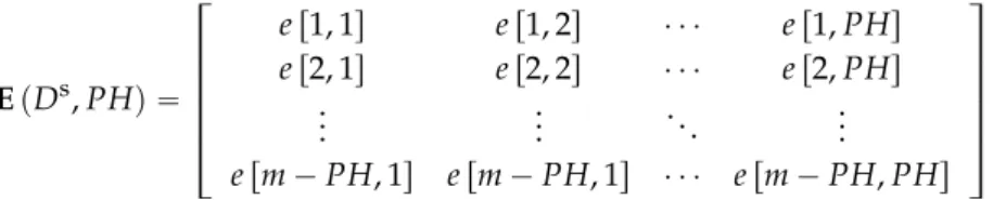
where ε`Dt˘ and ε pDgqdenote the root-mean-square errors (RMSE) of the training set Dtand the testing set Dg, respectively. Consider a given prediction horizon (PH) and a simulation set Ds(with m consecutive input-output pairs). Assuming that E pDs, PHq is an error matrix:
E pDs, PHq “ » — — — — – e r1, 1s e r1, 2s ¨ ¨ ¨ e r1, PHs e r2, 1s e r2, 2s ¨ ¨ ¨ e r2, PHs .. . ... . .. ... e rm ´ PH, 1s e rm ´ PH, 1s ¨ ¨ ¨ e rm ´ PH, PHs fi ffi ffi ffi ffi fl (5)
where e ri, js is the model prediction error taken from instant i of Dsat step j within the PH. By denoting ρ p., iq as the RMS function operating over the ithcolumn of its argument matrix, then ε pDs, PHq is
defined as: ε pDs, PHq “ PH ÿ i“1 ρ pE pDs, PHq , iq (6)
O pµq denotes the model complexity, which is equal to the number of input features + 1, multiplied by the number of hidden neurons, reflecting the RBF input-output topology.
The MOGA searches the space spanned by the number of neurons and the input features, i.e., the model structure. Each individual in the population has a chromosome representation consisting of two components. The first corresponds to the number of hidden neurons The second component is a string of integers, each one representing the index of a particular feature in F. The chromosome representation is shown in Figure5.
Energies 2016, 9, 57
In our work, the corresponding objectives for μ and μ were considered as follows:
g
p s t μ ε D ,?ε D , ?ε D PH, (3)
s μ O μ (4)where ε and ε denote the root‐mean‐square errors (RMSE) of the training set and the testing set , respectively. Consider a given prediction horizon (PH) and a simulation set Ds (with m consecutive input‐output pairs). Assuming that E
D PHs,
is an error matrix:
s 1,1 1, 2 1, 2,1 2, 2 2, , ,1 ,1 , e e e PH e e e PH D PH e m PH e m PH e m PH PH E (5)where e i j is the model prediction error taken from instant i of
, Ds at step j within the PH. By denoting ρ .,i as the RMS function operating over the i
th column of its argument matrix, then
s
ε D PH, is defined as:
s
1 s ρ , , ε , PH i D PH H i D P
E (6)μ denotes the model complexity, which is equal to the number of input features + 1, multiplied by the number of hidden neurons, reflecting the RBF input‐output topology. The MOGA searches the space spanned by the number of neurons and the input features, i.e., the model structure. Each individual in the population has a chromosome representation consisting of two components. The first corresponds to the number of hidden neurons The second component is a string of integers, each one representing the index of a particular feature in . The chromosome representation is shown in Figure 5.
Figure 5. Chromosome representation.
Before being evaluated in the MOGA, each model has its parameters determined by a Levenberg‐Marquardt algorithm [37] minimizing an error criterion that exploits the linear‐nonlinear relationship of the RBF NN model parameters [52–54]. The initial values of the nonlinear parameters (C and σ ) are chosen randomly, or with the use of a clustering algorithm, w is determined as a linear least‐squares solution, and the procedure is terminated using the early‐stopping approach [55] within a maximum number of iterations.
Figure 5.Chromosome representation.
Before being evaluated in the MOGA, each model has its parameters determined by a Levenberg-Marquardt algorithm [37] minimizing an error criterion that exploits the linear-nonlinear relationship of the RBF NN model parameters [52–54]. The initial values of the nonlinear parameters (C and σ) are chosen randomly, or with the use of a clustering algorithm, w is determined as a linear least-squares solution, and the procedure is terminated using the early-stopping approach [55] within a maximum number of iterations.
Energies 2016, 9, 57 11 of 24
4.3. Model Design Cycle
Briefly, the model design optimization problem is a sequence of actions which are undertaken by the model designer. These actions are repeated until the pre-specified design goals are achieved. There are three main actions in model design cycle: problem definition, solution(s) generation and analysis of results. In the problem definition stage, the datasets, the ranges of features and neurons are defined, as well as the objectives. After this stage, the MOGA does a guided search to obtain models that satisfy the predefined objectives and goals. In the third stage, the set of models obtained that lie in the Pareto front are analyzed. In this set, the performance of the models in the validation set (not involved in the design) is of paramount importance. If good solutions are found, the process stops. Otherwise, based on the results analysis, the search space can be reduced, and/or the objectives and goals can be redefined, therefore restricting the trade-off surface coverage. A more detailed description of the MOGA based ANN design framework can be found, for instance, in [43].
4.4. Data Preparation
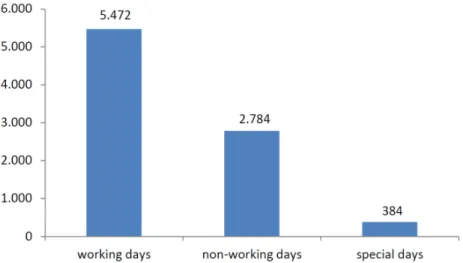
After an analysis of the original data, a new code was considered for the feature “day type”. The new code refers to “special days”. By comparing the amount of energy consumption for working and non-working days, it has been revealed that for some days over the years 2010 and 2011, the amount of energy consumption has an average value between working and non-working days. By comparing these special days with the Spanish calendar for both years, it was found that those days occurred in the early days of the year, or in working days which were located between national/regional holidays and weekends. Based on that, these special days received the code 0.5. Figure6shows the distribution of whole data samples in terms of “day type”.
Energies 2016, 9, 57 4.3. Model Design Cycle Briefly, the model design optimization problem is a sequence of actions which are undertaken by the model designer. These actions are repeated until the pre‐specified design goals are achieved. There are three main actions in model design cycle: problem definition, solution(s) generation and analysis of results. In the problem definition stage, the datasets, the ranges of features and neurons are defined, as well as the objectives. After this stage, the MOGA does a guided search to obtain models that satisfy the predefined objectives and goals. In the third stage, the set of models obtained that lie in the Pareto front are analyzed. In this set, the performance of the models in the validation set (not involved in the design) is of paramount importance. If good solutions are found, the process stops. Otherwise, based on the results analysis, the search space can be reduced, and/or the objectives and goals can be redefined, therefore restricting the trade‐off surface coverage. A more detailed description of the MOGA based ANN design framework can be found, for instance, in [43].
4.4. Data Preparation
After an analysis of the original data, a new code was considered for the feature “day type”. The new code refers to “special days”. By comparing the amount of energy consumption for working and non‐working days, it has been revealed that for some days over the years 2010 and 2011, the amount of energy consumption has an average value between working and non‐working days. By comparing these special days with the Spanish calendar for both years, it was found that those days occurred in the early days of the year, or in working days which were located between national/regional holidays and weekends. Based on that, these special days received the code 0.5. Figure 6 shows the distribution of whole data samples in terms of “day type”.
Figure 6. Distribution of original data samples in terms of day type from 1 September 2010 to 29
February 2012.
Since the original data was obtained with a sampling interval of 1 min, its size was too large (514,762 samples) to be handled by the MOGA framework, and was reduced in several stages. Due to presence of gaps in the data, there were 51 consecutive periods over the whole data. In the first stage, each period was divided into one week length segments. Based on these divisions, those durations whose length was less than two weeks were ignored in this work. This stage resulted into 13 periods containing at least two weeks of data. Table 4 shows the periods selected in the first stage. In the second stage, the data for all periods was reduced by a factor of 15 by averaging every 15 consecutive samples inside each segment. The sampling interval was then increased to 15 min.
Figure 6. Distribution of original data samples in terms of day type from 1 September 2010 to 29 February 2012.
Since the original data was obtained with a sampling interval of 1 min, its size was too large (514,762 samples) to be handled by the MOGA framework, and was reduced in several stages. Due to presence of gaps in the data, there were 51 consecutive periods over the whole data. In the first stage, each period was divided into one week length segments. Based on these divisions, those durations whose length was less than two weeks were ignored in this work. This stage resulted into 13 periods containing at least two weeks of data. Table4shows the periods selected in the first stage.
In the second stage, the data for all periods was reduced by a factor of 15 by averaging every 15 consecutive samples inside each segment. The sampling interval was then increased to 15 min.
Energies 2016, 9, 57 12 of 24
Table 4.The periods selected in the first stage.
Period Number Start End
1 2 September 2010 00:00:00 15 September 2010 23:59:00 2 24 September 2010 00:00:00 14 October 2010 23:59:00 3 9 November 2010 00:00:00 22 November 2010 23:59:00 4 27 December 2010 00:00:00 9 January 2011 23:59:00 5 11 January 2011 00:00:00 31 January 2011 23:59:00 6 9 February 2011 00:00:00 1 March 2011 23:59:00 7 11 March 2011 00:00:00 31 March 2011 23:59:00 8 2 June 2011 00:00:00 22 June 2011 23:59:00 9 8 July 2011 00:00:00 1 September 2011 23:59:00 10 14 October 2011 00:00:00 27 October 2011 23:59:00 11 5 November 2011 00:00:00 23 December 2011 23:59:00 12 29 December 2011 00:00:00 11 January 2012 23:59:00 13 19 January 2012 00:00:00 8 February 2012 23:59:00
In the third stage, by starting from the second week within each period, three random days along with the last seven consecutive days were selected as lags for each variable. This way, a data set D with 8640 samples was obtained. Figure7shows the distribution of samples of data set D in terms of “day type”.
Energies 2016, 9, 57
Table 4. The periods selected in the first stage.
Period Number Start End
1 2 September 2010 00:00:00 15 September 2010 23:59:00 2 24 September 2010 00:00:00 14 October 2010 23:59:00 3 9 November 2010 00:00:00 22 November 2010 23:59:00 4 27 December 2010 00:00:00 9 January 2011 23:59:00 5 11 January 2011 00:00:00 31 January 2011 23:59:00 6 9 February 2011 00:00:00 1 March 2011 23:59:00 7 11 March 2011 00:00:00 31 March 2011 23:59:00 8 2 June 2011 00:00:00 22 June 2011 23:59:00 9 8 July 2011 00:00:00 1 September 2011 23:59:00 10 14 October 2011 00:00:00 27 October 2011 23:59:00 11 5 November 2011 00:00:00 23 December 2011 23:59:00 12 29 December 2011 00:00:00 11 January 2012 23:59:00 13 19 January 2012 00:00:00 8 February 2012 23:59:00
In the third stage, by starting from the second week within each period, three random days along with the last seven consecutive days were selected as lags for each variable. This way, a data set with 8640 samples was obtained. Figure 7 shows the distribution of samples of data set D in terms of “day type”. Figure 7. Distribution of samples in data set D in terms of day type. 4.5. Design Experiments
Based on the model design cycle described in Section 4.3, several designs were conducted in such a way that their results led to the definition of a new design, by redefining variables and their corresponding lag terms, as well as imposing restrictions on objectives.
In a first step, we conducted designs with features requiring lag terms spread over at most 7 days. After analyzing and comparing the results with those obtained in [17], the spread of lags was reduced to cover at most 2 days, and finally to cover at most one day. Based on that, four new designs were carried out.
For all designs, data set D, stated in Section 4.4, containing 8640 samples was used. Since a sampling interval of 15 min was used, and the objective was to obtain forecasts of electric power 1 h‐ahead, a prediction horizon of four steps was employed. In this work, as in [17], two groups of models were considered. The first group contains simple models where only weather variables are used as exogenous variables. The second group considers complete models involving both weather
Figure 7.Distribution of samples in data set D in terms of day type.
4.5. Design Experiments
Based on the model design cycle described in Section4.3, several designs were conducted in such a way that their results led to the definition of a new design, by redefining variables and their corresponding lag terms, as well as imposing restrictions on objectives.
In a first step, we conducted designs with features requiring lag terms spread over at most 7 days. After analyzing and comparing the results with those obtained in [17], the spread of lags was reduced to cover at most 2 days, and finally to cover at most one day. Based on that, four new designs were carried out.
For all designs, data set D, stated in Section4.4, containing 8640 samples was used. Since a sampling interval of 15 min was used, and the objective was to obtain forecasts of electric power 1 h-ahead, a prediction horizon of four steps was employed. In this work, as in [17], two groups of models were considered. The first group contains simple models where only weather variables are used as exogenous variables. The second group considers complete models involving both weather and solar cooling operation variables. The list of candidate variables used and the range of lags for the design experiments are given in Tables5and6respectively.
Energies 2016, 9, 57 13 of 24
Table 5.List of variables used.
Variable Notation Unit Range in D
Electric power demand added up with the electric power
supplied by the PV plant x1 kW r11.73, 74.65s
Day type (working day/non-working day/semi-holidays) x2 - p0, 0.5, 1q
Outdoor temperature x3 ˝C r2.73, 43.79s
Outdoor solar radiation x4 W/m2 r0, 1127.81s
State of pump B1.1 (off/on) x5 - p0, 1q
State of Pump B1.2 (off/on) x6 - p0, 1q
State of Pump B2.1 (off/on) x7 - p0, 1q
State of Pump B2.2 (off/on) x8 - p0, 1q
State of Pump B7 (off/on) x9 - p0, 1q
State of the boiler (off/on) x10 - p0, 1q
State of the absorption machine (off/on) x11 - p0, 1q
State of the cooling tower (off/on) x12 - p0, 1q
State of the heat pump (off/on) x13 - p0, 1q
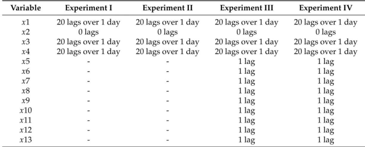
Table 6.Description of the lags used.
Variable Experiment I Experiment II Experiment III Experiment IV
x1 20 lags over 1 day 20 lags over 1 day 20 lags over 1 day 20 lags over 1 day
x2 0 lags 0 lags 0 lags 0 lags
x3 20 lags over 1 day 20 lags over 1 day 20 lags over 1 day 20 lags over 1 day x4 20 lags over 1 day 20 lags over 1 day 20 lags over 1 day 20 lags over 1 day
x5 - - 1 lag 1 lag x6 - - 1 lag 1 lag x7 - - 1 lag 1 lag x8 - - 1 lag 1 lag x9 - - 1 lag 1 lag x10 - - 1 lag 1 lag x11 - - 1 lag 1 lag x12 - - 1 lag 1 lag x13 - - 1 lag 1 lag
As it can be seen in Table6, Experiments I and II correspond to simple models in which only weather variables have been used; Experiments III and IV consider complete models. In Table6, “lag 0” for variable “day type” (x2) is translated into the day type of instant k ` 1 for which the electric power demand is predicted. In fact, weather and electric power demand variables are strongly related to their most recent values and also, to a certain extent, to their values 24 h before. As a result, for x1, x3 and x4 a heuristic, proposed in [43], was used to select 20 lags over one full day, in such a way that more recent values predominate in the set of searchable lags for these variables. Hence, based on this heuristic, the 20 lags used are r1–7, 9, 11, 13, 16, 20, 24, 29, 36, 43, 53, 65, 79, 96s . In this list, and as an example, lags 1 and 2 denote delays of 15 and 30 min, respectively. The objectives and the corresponding goals are given in Table7.
Table 7.Objectives and their corresponding restriction of experiments.
Objectives Experiment I Experiment II Experiment III Experiment IV
ε`Dt˘ Minimize <0.059 Minimize <0.054
ε pDgq Minimize <0.061 Minimize <0.052
ε pDs, 16q Minimize Minimize Minimize Minimize
Energies 2016, 9, 57 14 of 24
Regarding MOGA’s design framework parameters specification, for experiments I and III, the range rdm, dMs, where dmand dMare the minimum and maximum number of features, was set to
[1, 30] while for experiments II and IV they were set to [1, 15] and [1, 21], respectively. Similarly, for experiments I and III, the range rnm, nMs, where nmand nMare the minimum and maximum number
of neurons, was set to [2,30] while for experiments II and IV, these ranges were set to r1, 18s and r1, 21s, repectively. For all designs, the population size and the number of generations were set to 100. For each experiment, a proper sub dataset DWwas derived from data set D whose features are those columns of D which correspond to the lags defined in the corresponding experiment.
In order to generate training, testing and validation sets for each experiment, firstly the ApproxHull algorithm [56] was applied on corresponding DW to obtain convex points reflecting
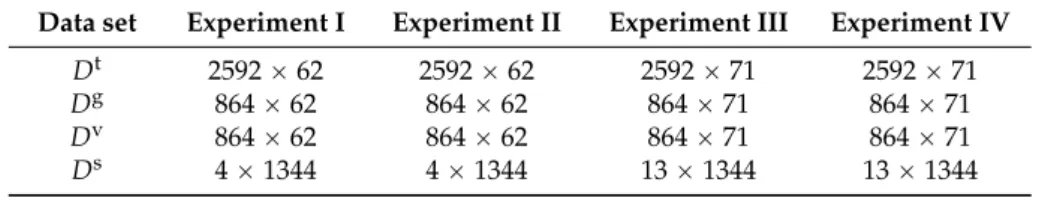
the whole input range in which the model is supposed to be used. Secondly, 50% of whole samples in DWwere used to generate training, testing and validation sets with proportions of 60%, 20% and 20%, respectively. In this step all convex points were incorporated in the training set. Afterwards, the remaining samples were shared randomly into the rest of the training set, and the testing and validation sets. Regarding the simulation dataset Ds, 1344 consecutive samples from 1 October 2010 00:00:00 to 14 October 2010 23:59:00 were considered. In this set, the rows correspond to the variables used, whose samples are in each column while, for the other sets, the number of rows correspond to the patterns, and the number of columns to the features. The size of training, testing and validation datasets as well as the simulation dataset of each experiment is given in Table8.
After one run of the MOGA for each experiment, the non-dominated and preferred sets of models were generated. In the case that no restriction is considered on objectives, the non-dominated set is the same as preferred set; otherwise, the preferred set is a subset of the non-dominated set whose solutions satisfy the goals. Please refer to [51] for further information about how the preferred set can be obtained from the non-dominated set by applying the preferably criterion. The number of models in non-dominated and preferred sets for each experiment is given in Table9.
Table 8.Size of training, testing and validation sets.
Data set Experiment I Experiment II Experiment III Experiment IV
Dt 2592 ˆ 62 2592 ˆ 62 2592 ˆ 71 2592 ˆ 71
Dg 864 ˆ 62 864 ˆ 62 864 ˆ 71 864 ˆ 71
Dv 864 ˆ 62 864 ˆ 62 864 ˆ 71 864 ˆ 71
Ds 4 ˆ 1344 4 ˆ 1344 13 ˆ 1344 13 ˆ 1344
Table 9.Size of non-dominated and preferred sets.
Experiment Non-dominated set Preferred set
Experiment I 346 346
Experiment II 238 88
Experiment III 289 289
Experiment IV 366 182
5. Results and Discussion
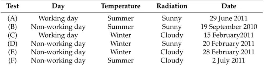
The models presented in this paper have been tested and compared by means of real data acquired at the CIESOL building. To do that, a battery of tests has been selected according to certain representative characteristics, such as, the type of day (working and non-working days), the season of the year and the quantity of solar radiation (sunny and cloudy days). A complete description of the battery of tests is shown in Table10. Furthermore, a prediction horizon over 1 h has been set mainly due to the energy price changes and the dynamic behaviour of indoor temperature [17].
Since in MOGA related experiments, the data used a sampling interval of 15 min, each test in Table10contains 96 samples. Moreover, the corresponding prediction horizon over 1 h is equal to
Energies 2016, 9, 57 15 of 24
four steps. For the model proposed in [17], each test includes 1440 samples due to the 1 min sampling rate. Hence, the corresponding prediction horizon over 1 h is equal to 60 steps. For convenience, the complete model proposed in [17] and the models obtained by MOGA will be denoted as PREVIOUS and MOGA models, respectively. In order to compare the MOGA models obtained from each experiment with the PREVIOUS model, one model was selected from the non-dominated/preferred set, with a good compromise between performance and complexity.
Table 10.Battery of tests performed.
Test Day Temperature Radiation Date
(A) Working day Summer Sunny 29 June 2011
(B) Non-working day Summer Sunny 19 September 2010
(C) Working day Winter Cloudy 15 February2011
(D) Non-working day Winter Sunny 20 February 2011
(E) Non-working day Winter Cloudy 28 February 2011
(F) Non-working day Summer Cloudy 2 July 2011
In our work, models I–IV were the selected MOGA models from experiments I–IV, respectively. Information about the selected MOGA models as well as the PREVIOUS is given in Table11. Using the notation of Table6, the formal description of models I–IV is given by Equations (7)–(10), respectively:
ˆy pk ` 1q “ f1px1pkq , . . . , x1pk ´ 6q , x1pk ´ 8q , x1pk ´ 11q , x1pk ´ 12q , x1pk ´ 19q , x2pk ` 1q , x3pk ´ 2q , x3pk ´ 7q , x3pk ´ 10q , x4pk ´ 4q , x4pk ´ 10q , x4pk ´ 17qq (7) ˆy pk ` 1q “ f2px1pkq , . . . , x1pk ´ 4q , x1pk ´ 6q , x1pk ´ 9q , x1pk ´ 10q , x1pk ´ 15q , x1pk ´ 18q , x3pk ´ 9q , x4pkq , x4pk ´ 8q , x4pk ´ 18qq (8) ˆy pk ` 1q “ f3px1pk ´ 1q , x1pk ´ 3q , x1pk ´ 4q , x1pk ´ 5q , x1pk ´ 7q , x1pk ´ 10q , x1pk ´ 11q , x1pk ´ 12q , x1pk ´ 14q , x1pk ´ 15q , x1pk ´ 16q , x2pk ` 1q , x3pkq , x3pk ´ 2q , x3pk ´ 3q , x3pk ´ 4q , x3pk ´ 8q , x3pk ´ 12q , x3pk ´ 13q , x3pk ´ 15q , x3pk ´ 16q , x4pk ´ 2q , x4pk ´ 3q , x4pk ´ 5q , x4pk ´ 7q , x4pk ´ 12q , x7pkq , x11pkq , x13pkqq (9) ˆy pk ` 1q “ f4px1pkq , x1pk ´ 1q , x1pk ´ 2q , x1pk ´ 3q , x1pk ´ 5q , x1pk ´ 17q , x2pk ` 1q , x3pk ´ 18q , x4pk ´ 3q , x4pk ´ 5q , x4pk ´ 10q , x4pk ´ 14q , x4pk ´ 15q , x4pk ´ 18q , x9pkq , x10pkq , x11pkq , x13pkqq (10)
ˆy pk ` 1q in Equations (7)–(10) is the output of the corresponding RBF neural network, representing o rks in Equation (2). Each function fj, tj “ 1, 2, 3, 4u has its own set of input terms. These input terms,
all together, constitute the input data sample at instant k corresponding to i rks in Equation (2).
Table 11.Selected multi objective genetic algorithm (MOGA) models and PREVIOUS model. Artificial neural networks: ANN.
Model Number of features Number of neurons Complexity
Model I 18 13 247
Model II 14 18 270
Model III 29 11 330
Model IV 18 20 380
NARX-ANN 67 10 680
To compare MOGA models with the PREVIOUS model over the battery of tests stated in Table10, five statistical criteria were considered: mean absolute error (MAE), mean relative error (MRE), Mean
Energies 2016, 9, 57 16 of 24
absolute percentage error (MAPE), maximum absolute error (MaxAE) and standard deviation of predicted values (σ). These criteria can be calculated according to Equations (11)–(15):
MAE “ 1 N N ÿ i“1 |x piq ´ ˆx piq| (11) MRE “ 1 N N ÿ i“1 |x piq ´ ˆx piq| x piq (12) MAPE “ 100% N N ÿ i“1 |x piq ´ˆx piq| |x piq| (13)
MaxAE “ max pAE px, ˆxqq (14)
σ “ g f f e1 N N ÿ i“1 ` ˆx piq ´ ˆx piq˘2 (15)
In Equations (11)–(15), N, x and ˆx denote the number of samples, measured values and predicted values of the variable, respectively. The evaluations of MOGA and PREVIOUS models over the battery of tests for a prediction horizon of 1 h are given in Tables12–17. The best values for each criterion are identified in bold.
Regarding test A, a working sunny day in summer, Model I, as a simple model, not only has minimum values in terms of MAE, MRE and MAPE among other MOGA models but also has a better performance than PREVIOUS in terms of these criteria. In this test, in overall, simple models I and II have better performance in comparison with complete models III and IV.
Table 12.Results obtained by MOGA and PREVIOUS models over Test A, for a prediction horizon (PH) of 1 h. Mean absolute error (MAE); mean relative error (MRE); mean absolute percentage error (MAPE); maximum absolute error (MaxAE).
Parameter Model I Model II Model III Model IV PREVIOUS
MAE (kW) 1.92 2.14 2.28 3.55 1.96
MRE (kW) 0.06 0.08 0.07 0.12 0.06
MAPE (%) 6.29 8.11 7.66 12.39 6.38
MaxAE (kW) 12.36 14.22 10.21 13.82 10.99
σ(kW) 8.92 7.86 8.91 6.99 7.17
Table 13.Results obtained by MOGA and PREVIOUS models over Test B, for a PH of 1 h.
Parameter Model I Model II Model III Model IV PREVIOUS
MAE (kW) 0.95 1.22 1.29 0.93 0.84
MRE (kW) 0.05 0.07 0.07 0.05 0.05
MAPE (%) 5.60 7.21 7.86 5.80 5.13
MaxAE (kW) 3.60 3.15 4.83 3.38 3.59
σ(kW) 2.01 2.48 1.78 1.75 1.52
Table 14.Results obtained by MOGA and PREVIOUS models over Test C, for a PH of 1 h.
Parameter Model I Model II Model III Model IV PREVIOUS
MAE (kW) 1.99 3.46 1.75 1.95 1.86
MRE (kW) 0.06 0.1 0.06 0.06 0.06
MAPE (%) 6.62 10.55 6.25 6.40 6.26
MaxAE (kW) 8.82 16.56 5.69 7.04 8.15
Energies 2016, 9, 57 17 of 24
Table 15.Results obtained by MOGA and PREVIOUS models over Test D, for a PH of 1 h.
Parameter Model I Model II Model III Model IV PREVIOUS
MAE (kW) 0.94 1.12 0.82 0.88 1.08
MRE (kW) 0.04 0.05 0.03 0.04 0.05
MAPE (%) 4.21 5.34 3.81 4.17 4.86
MaxAE (kW) 4.65 6.35 5.20 5.45 6.28
σ(kW) 1.95 1.64 1.08 1.72 1.52
Table 16.Results obtained by MOGA and PREVIOUS models over Test E, for a PH of 1 h.
Parameter Model I Model II Model III Model IV PREVIOUS
MAE (kW) 1.38 1.45 1.16 1.30 1.49
MRE (kW) 0.06 0.06 0.05 0.05 0.06
MAPE (%) 6.00 6.30 5.06 5.77 6.38
MaxAE (kW) 4.44 5.59 4.81 4.49 6.89
σ(kW) 1.80 1.39 1.28 1.65 1.43
Table 17.Results obtained by MOGA and PREVIOUS models over Test F, for a PH of 1 h.
Parameter Model I Model II Model III Model IV PREVIOUS
MAE (kW) 1.02 0.80 1.35 0.89 0.95
MRE (kW) 0.04 0.03 0.06 0.04 0.04
MAPE (%) 4.87 3.70 6.53 4.28 4.31
MaxAE (kW) 3.43 2.63 5.68 3.73 3.75
σ(kW) 1.95 1.99 1.44 1.97 1.88
With respect to test B, a non-working sunny day in summer, Model IV, as a complete model, has minimum values of MAE, MRE and σ in comparison with other MOGA models; with respect to MaxAE, it has a compromise performance between Model II and PREVIOUS.
In test C, a working cloudy day in winter, and in test D, a non-working sunny day in winter, the complete model III has minimum values in terms of MAE, MAPE and MaxAE among all models. Model I, a simple model, has also a good performance; actually better in 4 criteria than the complete PREVIOUS model, in test D.
In test E, a non-working cloudy day in winter, both simple and complete MOGA models have lower values in terms of MAE, MAPE and MaxAE than the PREVIOUS model. Model III has better performance in all criteria.
Regarding test F, a non-working cloudy day in summer, simple model II and complete model IV have better performance in terms of MAE, MAPE and MaxAE than PREVIOUS model. In this comparison, model II has minimum values in all criteria, except σ.
According to Tables12–17in the group of simple models, model I, in most cases, has better performance than model II. In the group of complete models, model III, in most cases, is better than model IV. Figures8–10show the comparison between measured and predicted value of electric power demand in CIESOL building, over tests A–F for a prediction horizon of 1 h, for the PREVIOUS model, model I and III, respectively.
Comparing the performance of all MOGA models over the battery of tests, in general complete models III and IV have a better performance in winter than in summer, while simple model I has a compromise performance between summer and winter.