Implementing an integrated syntax directed editor for LISS

(1)

Universidade do Minho Escola de Engenharia Departamento de Inform´atica

Damien da Silva Vaz

Implementing an Integrated Syntax

Directed Editor for LISS.

(2)

Escola de Engenharia Departamento de Inform´atica

Damien da Silva Vaz

Implementing an Integrated Syntax

Directed Editor for LISS.

Master dissertation

Master Degree in Computer Science

Dissertation supervised by

Professor Pedro Rangel Henriques Professor Daniela da Cruz

(3)

A C K N O W L E D G E M E N T S

First, I would like to thank my supervisor Pedro Rangel Henriques and co-supervisor Daniela da Cruz. They are the most who supported me throw this ambitious project and took me to the final stage of my university career.

Thank you also to my family (particularly, my brother Jo¨el and my father Celestino) and friends (Ranim, Bruno, Chlo´e, Tiago, Saozita, Nuno, David, Juliette, Jessica) for supporting me.

And last but not least, I would like to dedicate this thesis to my, particularly, most beautiful mother. Despite you couldn’t be here to watch me conclude my studies. Wherever you are, I hope that you are proud of me. None of this could have been made without their unconditional help.

(4)

The aim of this master work is to implement LISS language in ANTLR compiler generator system using an attribute grammar which create an abstract syntax tree (AST) and generate MIPS assembly code for MARS (MIPS Assembler and Runtime Simulator) . Using that AST, it is possible to create a Syntax Directed Editor (SDE) in order to provide the typical help of a structured editor which controls the writing according to language syntax as defined by the underlying context free grammar.

(5)

R E S U M O

O tema desta dissertação é implementar a linguagem LISS em ANTLR com um gramática de atributos e no qual, irá criar uma árvore sintática abstrata e gerar MIPS assembly c ódigo para MARS (MIPS Assembler and Runtime Simulator). Usando esta árvore sintática ab-strata, criaremos uma SDE (Editor Dirigido a Sintaxe) no qual fornecerá toda a ajuda t´ıpica de um editor estruturado que controlará a escrita de acordo com a gramática.

(6)

1 i n t r o d u c t i o n 1

1.1 Objectives 1

1.2 Research Hypothesis 2

1.3 Document Structure 2

2 l i s s l a n g ua g e 3

2.1 Formal languages and grammar 3

2.2 LISS Data types 5

2.2.1 LISS lexical conventions 11

2.3 LISS blocks and statements 12

2.3.1 LISS declarations 13

2.3.2 LISS statements 13

2.3.3 LISS control statements 17

2.3.4 Other statements 21

2.4 LISS subprograms 22

2.5 Evolution of LISS syntax 24

3 ta r g e t m a c h i n e: mips 26

3.1 MIPS coprocessors 27

3.2 MIPS cpu data formats 28

3.3 MIPS registers usage 28

3.4 MIPS instruction formats 31

3.4.1 MIPS R-Type 31

3.4.2 MIPS I-Type 33

3.4.3 MIPS J-Type 35

3.5 MIPS assembly language 36

3.5.1 MIPS data declarations 36

3.5.2 MIPS text declarations 37

3.6 MIPS instructions 39

3.7 MIPS Memory Management 42

3.7.1 MIPS stack 42

3.7.2 MIPS heap 43

3.8 MIPS simulator 43

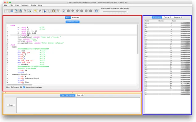
3.8.1 MARS at a glance 44

(7)

Contents

4.2 Lexical and syntatical analysis 49

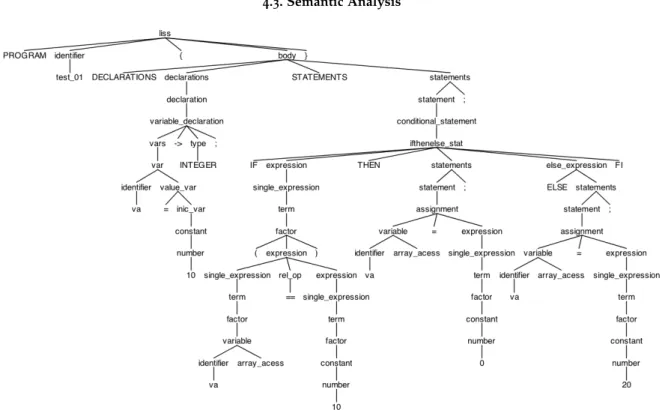
4.3 Semantic Analysis 50

4.3.1 Symbol Table 50

4.3.2 Error table in LISS 57

4.3.3 Types of error message 59

4.3.4 Validations Implemented 61

4.4 Code Generation 75

4.4.1 Strategy used for the code generation 75

4.4.2 LISS language code generation 84

4.4.3 Creating a variable in LISS 84

4.4.4 Loading a variable or a value 100

4.4.5 Assigning in LISS 101

4.4.6 Set operations 108

4.4.7 Sequence operations 109

4.4.8 Implementing Function calls 111

4.4.9 Implementing Input/Output 112

4.4.10 Implementing Conditional statements 114 4.4.11 Implementing Iterative statements 116 4.4.12 Implementing increment or decrement operators 121

5 s d e: development 123

5.1 What is a template? 124

5.2 Conception of the SDE 125

5.2.1 Toolbar meaning 127

5.2.2 Creating a program 129

5.2.3 Executing a program 139

5.2.4 Error System in liss|SDE 139

6 c o n c l u s i o n 141

6.1 Future Work 143

(8)

Figure 1 CFG example1

4

Figure 2 MIPS architecture 27

Figure 3 MIPS register 30

Figure 4 MARS GUI 44

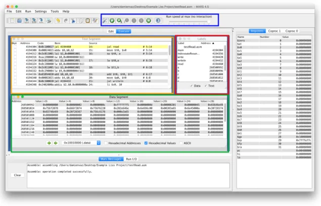
Figure 5 MARS GUI (Execution mode) 45

Figure 6 Traditional compiler 48

Figure 7 AST representation 50

Figure 8 Example of hierarchical symbol table 51

Figure 9 Global symbol table in LISS 52

Figure 10 InfoIdentifiersTable structure 56

Figure 11 ErrorTable structure 58

Figure 12 ErrorTable structure instantiated for example in Listing 4.5 59

Figure 13 Stack structure 81

Figure 14 Structure for saving information of each value declared in a array 87

Figure 15 Array structure with size 2,2,3. 89

Figure 16 Set structure in JAVA 92

Figure 17 Set structure in JAVA 92

Figure 18 Architecture of the stack relatively to a function in LISS 96 Figure 19 Schema of the conditional statements in LISS 114 Figure 20 Schema of the for-loop statement using the condition ’in’ 117 Figure 21 Schema of the for-loop statement using the condition ’inArray’ 119

Figure 22 Schema of the while-loop statement 120

Figure 23 Example of an IDE visual interface (XCode)2

123

Figure 24 SDE example 125

Figure 25 liss|SDE 126

Figure 26 liss|SDE structure 127

Figure 27 Toolbar of liss|SDE 127

Figure 28 File option of toolbar in liss|SDE 128 Figure 29 Run option of toolbar in liss|SDE 128 Figure 30 Help option of toolbar in liss|SDE 128 Figure 31 About option of toolbar in liss|SDE 129

(9)

List of Figures

Figure 32 Creating a LISS program (1/17) 130

Figure 49 Flow of the execution of a liss code in the liss|SDE 139 Figure 50 Output of the execution of the HelloWorld program 139

(10)

Table 1 LISS data types 6

Table 2 Operations and signatures in LISS 7

Table 3 MIPS registers 28

Table 4 R-Type binary machine code 32

Table 5 Transformation of R-Type instruction to machine code 33

Table 6 Distinct I-Type instruction formats 34

Table 7 Immediate (I-Type) Imm16 instruction format 34 Table 8 Immediate (I-Type) Off21 instruction format 34 Table 9 Immediate (I-Type) Off26 instruction format 35 Table 10 Immediate (I-Type) Off11 instruction format 35 Table 11 Immediate (I-type) Off9 instruction format 35

Table 12 J-Type instruction format 35

Table 13 Example of Data transfer instruction in MIPS 39 Table 14 Example of Arithmetic instruction in MIPS 40 Table 15 Example of Logical instruction in MIPS 40 Table 16 Example of Bitwise Shift instruction in MIPS 40 Table 17 Example of Conditional Branch instruction in MIPS 41 Table 18 Example of Unconditional Branch instruction in MIPS 41 Table 19 Example of Pseudo Instructions in MIPS 41 Table 20 Example of SYSCALL instruction in MIPS 42

Table 21 TYPE category information 53

Table 22 ST information for an integer variable 53 Table 23 ST information for a boolean variable 54

Table 24 ST information for an array variable 54

Table 25 ST information for a set variable 54

Table 26 ST information for a sequence variable 55

Table 27 ST information for a function 55

Table 28 Types of error message in LISS 60

(11)

(12)

1

I N T R O D U C T I O N

In informatics, solving problems with computers is related to the necessity of helping the end-users, facilitating their life. And all these necessities pass through developers who creates programs for this purpose.

However, developing programs is a difficult task; analyzing problems, and debugging software takes effort and time.

And this is why we must find a solution for these problems.

Developing a software package requires tools to help the developers to maximize their programming productivity. These tools are: on one hand, compilers to generate lower-level code (machine code) from the level source code (the input program written in an high-level programming language); on the other hand, editors to create that source code. And to make easier and safer the programmers work, high-level programming languages were created for facilitating their work.

This is not enough to overcome all the difficulties for creating a program in a safety way and having a high level productivity!

This is why we need to have fresh ideas and to implement more features to help on solving these problems.

1.1 o b j e c t i v e s

In this work, this project aims to develop an editor with the concept of a SDE (Syntax Directed Editor).

It is intended that the editor works with language designed by the members of the Lan-guage Processing group at UM which is called LISS.

LISS language will be specified by an attribute grammar that will be passed, as input, to ANTLR. The compiler generated by ANTLR will generate MIPS assembly code (lower-level source code).

The front-end and the back-end of that compiler will be explained and detailed along the next pages.

(13)

1.2. Research Hypothesis

1.2 r e s e a r c h h y p o t h e s i s

It is possible to synthesize a complete source program, ready to be compiled and executed, selecting the appropriate alternative language constructors and writing literals in the right positions in a special editor guided by the source language structure, or syntax.

1.3 d o c u m e n t s t r u c t u r e

In this section, the project planned for this master thesis will be explained. First, create an ANTLR version of the CFG grammar for LISS language.

Second, extend the LISS CFG to an AG in order to specify throw it the generation of MIPS assembly code. Then verify the correctness of the assembly code generated with a simple MIPS simulator, named MARS, that will be selected to provide all the tools for checking it. Third, the desired Structure-Editor, SDE, will be developed based on ANTLR. It will be implemented with Java (JAVAFX) because ANTLR has always been implemented via Java and it is said, also, to use Java target as a reference implementation mirrored by other targets. At this phase, we will create an IDE similar to other platforms but with the capacity of being a syntax-directed editor.

Finally, exhaustive and relevant tests will be made with the tool created and, the out-comes will be analyzed and discussed.

(14)

2

L I S S L A N G U A G E

LISS (da Cruz and Henriques, 2007a) -that stands for Language of Integers, Sequences

and Sets- is an imperative programming language, defined by the Language Processing members (Pedro Henriques and Leonor Barroca) at UM for teaching purposes (compiler course).

The idea behind the design of LISS language was to create a simplified version of the more usual imperative languages although combining functionalities from various lan-guages.

It is designed to have atomic or structured integer values, as well as, control statements and block structure statements.

Before explaining the basic statements of the language and its data types using a context free grammar, let’s remember briefly the basilar concepts related to formal programming languages and their definition using grammars (context free and attribute grammars).

2.1 f o r m a l l a n g ua g e s a n d g r a m m a r

A grammar (Chomsky,1962;Gaudel,1983;Waite and Goos,1984;Aho et al.,1986;Kastens, 1991b; Muchnick, 1997; Hopcroft et al.,2006;Grune et al.,2012) is a set of derivation rules

(or production) that explains how words are used to build the sentences of a language. A grammar (Deransart et al.,1988;Alblas,1991;Kastens,1991a;Swierstra and Vogt,1991; Deransart and Jourdan, 1990; Räihä, 1980;Filè,1983; Oliveira et al., 2010) is considered to

be a language generator and also a language recognizer (checking if a sentence is correctly derived from the grammar).

The rules describe how a string is formed using the language alphabet, defining the sentences that are valid according to the language syntax.

One of the most important researchers in this area was Noam Chomsky. He defined the notion of grammar in computer science’s field.

He described that a formal grammar is composed by a finite set of production rules (left hand side 7→right hand side)

(15)

2.1. Formal languages and grammar

These symbols are split into two sets : non terminals, terminals; the start symbol is a special non-terminal.

There is, always, at least one rule for the start symbol (see Figure 1) followed by other rules to derive each non-terminal. The non terminals are symbols which can be replaced and terminals are symbols which cannot be.

Figure 1.: CFG example1

One valid sentences (Example in Figure 1), could be : bbebee .

In the compilers area two major classes of grammars are used : CFG (Context-free gram-mar) and AG ( Attribute Gramgram-mar).

The difference between these two grammars are that a CFG is directed to define the syntax (only) and, AG contains semantic and syntax rules.

An AG is , basically, a GFC grammar extended with semantic definitions. It is a formal way to define attributes for the symbols that occur in each production of the underlying grammar. We can associate values to these attributes later, after processed with a parser; the evaluation will occur applying those semantic definition to any node of the abstract syntax tree. These attributes are divided into two groups: synthesized attributes and inherited attributes.

The synthesized attributes are the result of the attribute evaluation rules for the root sym-bol of each subtree, and may also use the values of the inherited attributes. The inherited attributes are passed down from parent nodes to children or between siblings.

Like that it is possible to transport information anywhere in the abstract syntax tree which is one of the strength for using an AG.

(16)

2.2 l i s s d ata t y p e s

There are 5 types available. From atomic to structured types, they are known as : integer, boolean, array, set and sequence.

Used for declaring a variable in a program, the data type gives us vital information for understanding what kind of value we are dealing with.

Let’s obverse a LISS code example:

1 a −> i n t e g e r ;

2 b −> boolean ;

3 c −> a r r a y s i z e 5 , 4 ; 4 d −> s e t ;

5 e −> sequence ;

Listing 2.1: Declaring a variable in LISS

As we can see in Listing 2.1, some variables (’a’,’b’,’c’,’d’ and ’e’) are being declared each one associated to a type (’integer’, ’boolean’, ’array’, ’set’ and ’sequence’). Syntactically, in LISS, this is done by writing the variable name followed by an arrow and the type of the variable (see Listing 2.2).

1 v a r i a b l e d e c l a r a t i o n : v a r s ’−>’ type ’ ; ’ 2 ; 3 v a r s : var ( ’ , ’ var ) ∗ 4 ; 5 var : i d e n t i f i e r v a l u e v a r 6 ; 7 v a l u e v a r : 8 | ’ = ’ i n i c v a r 9 ; 10 type : ’ i n t e g e r ’ 11 | ’ boolean ’ 12 | ’ s e t ’ 13 | ’ sequence ’ 14 | ’ a r r a y ’ ’ s i z e ’ dimension 15 ;

16 dimension : number ( ’ , ’ number ) ∗

17 ; 18 i n i c v a r : c o n s t a n t 19 | a r r a y d e f i n i t i o n 20 | s e t d e f i n i t i o n 21 | s e q u e n c e d e f i n i t i o n 22 ;

(17)

2.2. LISS Data types

Table 1.: LISS data types

Type Default Value

boolean false integer 0 array [0,...,0] set {} sequence nil 24 | ’ t r u e ’ 25 | ’ f a l s e ’ 26 ; 27 s i g n : 28 | ’ + ’ 29 | ’−’ 30 ;

Listing 2.2: CFG for declaring a variable in LISS

(18)

Table 2.: Operations and signatures in LISS

Operators && Functions Signatures

+ (add) integer x integer -> integer

- (subtract) integer x integer -> integer

||(or) boolean x boolean -> boolean

++ (union) set x set -> set

/ (division) integer x integer -> integer

* (multiply) integer x integer -> integer

&& (and) boolean x boolean -> boolean

** (intersection) set x set -> set

== (equal) integer x integer -> integer; boolean x boolean -> boolean != (not equal) integer x integer -> integer; boolean x boolean -> boolean

<(less than) integer x integer -> boolean

>(greater than) integer x integer -> boolean

<= (less than or equal to) integer x integer -> boolean >= (great than or equal to) integer x integer -> boolean

in (contains) integer x set -> boolean

tail sequence -> sequence

head sequence -> integer

cons integer x sequence -> sequence

delete integer x sequence -> sequence

copy sequence x sequence -> void

cat sequence x sequence -> void

isEmpty sequence -> boolean

length sequence -> integer

isMember integer x sequence -> boolean

Additionally, we may change the default values of the variables by initializing them with a different value (see an example in Listing 2.3). This can be made by writing an equal symbol after the variable name and, then, inserting the right value according to the type (see example in Listing 2.2).

1 a = 4 , b −> i n t e g e r ;

2 t = t r u e −> boolean ;

3 v e c t o r 1 = [ 1 , 2 , 3 ] , v e c t o r 2 −> a r r a y s i z e 5 ;

4 a = { x | x<10} −> s e t ;

5 seq1 = < <10 ,20 ,30 ,40 ,50 > > , seq3 = <<1,2>>, seq2 −> sequence ;

Listing 2.3: Initialize a variable

Now, let’s define which types are, correctly, associated with the arithmetic operators and functions in LISS (see Table 2).

(19)

So, in Table 2, we list the operators and functions, available in LISS, and their signa-ture. In order to understand the table better, we will explain how to read the table and its signature with one example.

Consider the symbol ’+’ (Table 2), indicates that both operands must be of type integer. The result of that operation, indicated by the symbol ’->’, will be an integer. Semantically, operations must be valid according to Table 2; otherwise the operations would be incorrect and throw an error.

Arrays. LISS supports a way of indexing a collection of integer values such that each value is uniquely addressed. LISS also supports an important property of multidimension-ality.

Called as ’array’, it is considered to be a static structured type due to the fact that its dimensions and maximum size of elements in each dimension is fixed at the declaration time.

The operations defined over arrays are: 1. indexing

2. assignment

Arrays can be initialized, in the declaration section, partially or completely in each di-mension. For example, consider an array of dimension 3x2 declared in the following way:

1 a r r a y 1 = [ [ 1 , 2 ] , [ 5 ] ] −> a r r a y s i z e 3 , 2 ;

Thi is equivalent to the initialization below:

1 a r r a y 1 = [ [ 1 , 2 ] , [ 5 , 0 ] , [ 0 , 0 ] ] −> a r r a y s i z e 3 , 2 ;

Notice that the elements that are not explicitly assigned, are initialized with the value 0 (see Table 1).

The grammar for array declaration and initialization is shown below.

1 a r r a y d e f i n i t i o n : ’ [ ’ a r r a y i n i t i a l i z a t i o n ’ ] ’ 2 ; 3 4 a r r a y i n i t i a l i z a t i o n : elem ( ’ , ’ elem ) ∗ 5 ; 6 7 elem : number

(20)

8 | a r r a y d e f i n i t i o n

9 ;

Sets. The type set, in LISS, is a collection of integers with no repeated numbers.

It is defined by an expression, in a comprehension, instead of by enumeration of its element. A set variable can have an empty value and, syntactically, this is done by writing ’{}’.

To define a set by comprehension, the free variable and the expression shall be return between curly brackets. The ’identifier’ (free variable) is separated from the expression by an explicit symbol ’|’.

The expression is built up from relational and boolean operators to define an integer interval.

The operations defined for sets are : 1. union

2. intersection 3. in (membership)

Let’s see an example of its syntax below:

1 s e t 1 = {x | x < 6 && x > −7} −> s e t ;

This declaration defines a set including all the integers from -7 to 6 (open interval) and other numbers are not included in the set.

The syntax for set declaration and initialization is :

1 s e t d e f i n i t i o n : ’ { ’ s e t i n i t i a l i z a t i o n ’ } ’ 2 ; 3 4 s e t i n i t i a l i z a t i o n : 5 | i d e n t i f i e r ’ | ’ e x p r e s s i o n 6 ;

(21)

Sequences. Considered as a dynamic array of one dimension, the type sequence is a list of ordered integers. But, in opposition to the concept of an array, its size is not fixed; this means that it grows dinamicallly at run time like a linked list. A sequence can have the empty value (syntactically done by writing ’<<>>’). If not empty, the sequence value is defined by enumerating its components (integers) in the right order. Let’s see deeper with one example:

1 c=<<1,2,3>> −> sequence ;

Listing 2.4: Example of valid operations using sequence on LISS

In the example of Listing 2.4the sequence is defined by three numbers (3,2,1). The operations defined for the sequence are:

1. tail (all the elements but the first) 2. head (the first element of the sequence)

3. cons (adds an element in the head of the sequence) 4. delete (remove a given element from the sequence) 5. copy (copies all the elements to another sequence)

6. cat (concatenates the second sequence at the end of the first sequence) 7. isEmpty (true if the sequence is empty)

8. length (number of elements of the sequence)

9. isMember (true if the number is an element of the sequence) Those operations will be explained further and deeper.

The grammar below defines how to declare a sequence:

1 s e q u e n c e d e f i n i t i o n : ’<< ’ s e q u e n c e i n i t i a l i z a t i o n ’>> ’ 2 ; 3 4 s e q u e n c e i n i t i a l i z a t i o n : 5 | v a l u e s 6 ; 7 8 v a l u e s : number ( ’ , ’ number ) ∗ 9 ;

(22)

2.2.1 LISS lexical conventions

Once you’ve declared a variable of a certain type, you cannot redeclare it again with the same name.

The variable name must be unique (see Listing 2.5).

1 program s i n g l e v a r i a b l e n a m e { 2 d e c l a r a t i o n s 3 i n t =1 −> i n t e g e r ; 4 i n t = t r u e −> boolean ; / / c a n n o t d e c l a r e t h i s v a r i a b l e w i t h t h i s name ( a l r e a d y e x i s t s ) 5 s t a t e m e n t s 6 }

Listing 2.5: Conflicts with variable names

Keywords cannot be used as variable names.

For example, you cannot declare a variable with the name array due to the fact that array is a keyword in LISS (in this case, a type).

See the example in Listing 2.6.

1 a r r a y −> a r r a y s i z e 3 , 4 ; / / v a r i a b l e ’ a r r a y ’ c a n n o t b e d e c l a r e d a s a

name

2 i n t e g e r −> i n t e g e r ;

Listing 2.6: Conflicts with keyword names

Variable names contain only letters and numbers, or the underscore sign. However the first character of the variable name must be a letter (lower or upper case). See the example below:

1 M y v a r i a b l e 1

2 MyVariable1

Numbers are composed of digits (one or more). Nothing more is allowed. See example below:

1 1 5 6 2

2 1

A string is a sequence of n-characters enclosed by double quotes. See example below:

(23)

2.3. LISS blocks and statements

2.3 l i s s b l o c k s a n d s tat e m e n t s

A LISS program is always composed of two parts: declarations and statements (a program block). LISS language is structured with a simple hierarchy. And this is done by structuring LISS code as a block.

Any program begins with a name then appear the declaration of variables and subpro-grams. After that appear the flow of the program by writing statements.

Let’s see one example (see Listing 2.7).

1 program sum{ 2 d e c l a r a t i o n s 3 i n t =2 −> i n t e g e r ; 4 s t a t e m e n t s 5 w r i t e l n ( i n t +3) ; 6 }

Listing 2.7: The structure of a LISS program (example)

So a program in LISS begins by, syntactically, writing ’program’ and then the name of the program (in this case, the name is ’sum’). A pair of curly braces delimits the contents of the program; that is done by opening it after the name of the program and closing it at the end of the program. After the left brace, appear the declaration and statement blocks.

As in a traditional imperative language (let’s compare ’C language’), if we don’t take the habit of declaring the variable always in a certain part of the code, it becomes confusing. This makes the programmer’s life harder to understand the code when the code is quite long.

So, in LISS, we always declare variables first (syntactically written by ’declarations’) and then the statements (syntactically written by ’statements’). This is due to the fact that LISS wants to help the user to create solid and correct code. And in this case, the user will always know that all the variable declarations will be always at the top of the statements and not randomly everywhere (see grammar in Listing 2.8).

1 l i s s : ’ program ’ i d e n t i f i e r body 2 ; 3 4 body : ’ { ’ 5 ’ d e c l a r a t i o n s ’ d e c l a r a t i o n s 6 ’ s t a t e m e n t s ’ s t a t e m e n t s 7 ’ } ’ 8 ;

(24)

2.3.1 LISS declarations

The declaration part is divided into two other parts: variable declarations and subprogram declarations, both optional.

The first part is explained in section 2.2; the subprogram part will be discussed later in section 2.4.

This part is specified by the following grammar (see Listing 2.9).

1 d e c l a r a t i o n s : v a r i a b l e d e c l a r a t i o n ∗ s u b p r o g r a m d e f i n i t i o n ∗

2 ;

Listing 2.9: CFG for declarations in LISS

2.3.2 LISS statements

As said previously, under the statements part, we control and implement the flow of a LISS program. In LISS, we may write none or, one or more statements consecutively.

Every statement ends with a semicolon, unless two type of statements (conditional and cyclic statements) as shown in Listing 2.10.

Listing 2.10: CFG for statements in LISS

Let’s see one example of a LISS program which shows how the language shall be used (see Listing 2.11).

1 program f a c t o r i a l { 2 d e c l a r a t i o n s

3 r e s =1 , i −> i n t e g e r ;

(25)

2.3. LISS blocks and statements 6 f o r ( j i n 1 . . i ) { 7 r e s = r e s ∗ j ; 8 } 9 w r i t e l n ( r e s ) ; 10 }

Listing 2.11: Example of using statements in LISS

Assignment. This statement assigns, as it is called, values to a variable and it is defined for every type available on LISS. This operation is done by writing the symbol ”=” in which a variable is assigned to the left side of the symbol and a value to the right side of the symbol.

Notice that an assignment requires that the variable on the left and the expression on the right must agree in type.

Let’s see in Listing 2.12an example.

1 program assignment1 { 2 d e c l a r a t i o n s 3 intA −> i n t e g e r ; 4 bool −> boolean ; 5 s t a t e m e n t s 6 intA = −3 + 5 ∗ 9 ; 7 bool = 2 < 8 ; 8 }

Listing 2.12: Example of assignment in LISS

In Listing 2.12, we can see assignment statements of integers and boolean types. Those assignments are correct, as noticed in the previous paragraphs, because they have the same type on the left and right side of the symbol equals (operations of integers assigned to a variable of integer type and operation of booleans assigned to a variable of boolean type).

The grammar that rules the assignment is shown at Listing 2.13.

1 assignment : d e s i g n a t o r ’ = ’ e x p r e s s i o n

2 ;

Listing 2.13: CFG for assignment in LISS

I/O.The input and output statements are also available in LISS.

The read operations, called syntactically as ’input’ in LISS, assign a value to a variable obtained from the standard input and require to be an atomic value (in this case, only an integer value).

(26)

2 d e c l a r a t i o n s

3 myInteger −> i n t e g e r ;

4 s t a t e m e n t s

5 i np ut ( myInteger ) ;

6 }

Listing 2.14: Example of input operation in LISS

Notice that, in Listing 2.14, the variable myInteger must be declared and must be integer otherwise the operations fails. The grammar that rules the input statement, is shown in Listing 2.15.

1 r e a d s t a t e m e n t : ’ in pu t ’ ’ ( ’ i d e n t i f i e r ’ ) ’

2 ;

Listing 2.15: CFG for input operation in LISS

The write operations, called syntactically as ’write’ or ’writeln’ in LISS, print an integer value in the standard output. Notice that ’write’ operation only prints the value and doesn’t move to a new line; instead, ’writeln’ moves to a new line at the end.

Listing 2.16shows some more examples.

1 w r i t e l n ( 4 ∗ 3 ) ; 2 w r i t e l n ( 2 ) ; 3 w r i t e l n ( ) ;

Listing 2.16: Example of output operations in LISS

Note that the write statement may have as assignment, an atomic value as well as an empty value or some complex arithmetic expression (see grammar in 2.17).

1 w r i t e s t a t e m e n t : w r i t e e x p r ’ ( ’ p r i n t w h a t ’ ) ’ 2 ; 3 4 w r i t e e x p r : ’ w r i t e ’ 5 | ’ w r i t e l n ’ 6 ; 7 8 p r i n t w h a t : 9 | e x p r e s s i o n 10 ;

(27)

Function call. The function call is a statement that is available for using the functions created in the program under the section ’declarations’ (as described in Section 2.3.1). This will allow reusing functions that were created by calling them instead of creating duplicated code.

See Listing 2.18 for a complete example.

1 program SubPrg { 2 3 d e c l a r a t i o n s 4 5 a = 4 , b= 5 , c= 5 −> i n t e g e r ; 6 d = [ 1 0 , 2 0 , 3 0 , 4 0 ] , ev −> a r r a y s i z e 4 ; 7 8 9 subprogram c a l c u l a t e ( ) −> i n t e g e r 10 { 11 d e c l a r a t i o n s 12 f a c = 6 −> i n t e g e r ; 13 r e s = −16 −> i n t e g e r ; 14 15 subprogram f a c t o r i a l ( n −> i n t e g e r ; m−> a r r a y s i z e 4 ) −> i n t e g e r 16 { 17 d e c l a r a t i o n s 18 r e s = 1 −> i n t e g e r ; 19 s t a t e m e n t s 20 while ( n > 0 ) 21 { 22 r e s = r e s ∗ n ; 23 n = n −1; 24 } 25 26 f o r ( a i n 0 . . 3 ) stepUp 1 27 { 28 d [ a ] = a∗ r e s ; 29 } 30 r e t u r n r e s ; 31 } 32 s t a t e m e n t s 33 r e s = f a c t o r i a l ( f a c , d ) ; 34 r e t u r n r e s / 2 ; 35 } 36 37 38 s t a t e m e n t s

(28)

39

40 a = c a l c u l a t e ( ) ; 41 w r i t e l n ( a ) ; 42 w r i t e l n ( d ) ; 43 }

Listing 2.18: Example of call function in LISS

In Listing 2.18, we can see that the function calculate(), called in the main program, and that is created under the declarations section.

The grammar who rules the function call is shown in Listing 2.19.

1 f u n c t i o n c a l l : i d e n t i f i e r ’ ( ’ s u b p r g a r g s ’ ) ’ 2 ; 3 s u b p r g a r g s : 4 | a r g s 5 ; 6 a r g s : e x p r e s s i o n ( ’ , ’ e x p r e s s i o n ) ∗ 7 ;

Listing 2.19: CFG for call function in LISS

2.3.3 LISS control statements

LISS language includes some statements for controlling the execution flow at runtime with two different kind of behaviour.

The first one is called conditional statement and it has only one variant in LISS language (see Listing 2.20).

The second one is called cyclic statement or iterative statement, and it has two variants (see Listing 2.20). 1 c o n d i t i o n a l s t a t e m e n t : i f t h e n e l s e s t a t 2 ; 3 i t e r a t i v e s t a t e m e n t : f o r s t a t 4 | w h i l e s t a t 5 ;

Listing 2.20: CFG for control statement in LISS

These control statements, mimics the syntax and the behaviour of other modern impera-tive language.

(29)

c o n d i t i o na l The if-statement, which is common across many modern programming languages, performs different actions according to decision depending on the truth value of a control conditional expression: an alternative ’else’ block is also allowed (optional).

If the conditional expression evaluates ’true’, the content of ’then’ block will be executed. Otherwise, if the condition is ’false’, the ’then’ block is ignored; and if an ’else’ block is provided it will be executed alternatively.

Let’s see an example in Listing 2.21.

1 i f ( y==x ) 2 then { 3 x=x + 1 ; 4 } e l s e { 5 x=x + 2 ; 6 }

Listing 2.21: LISS syntax of a if statement

The code shown in Listing 2.21, means that the if-statement evaluates the conditional expression ’y==x’. If the expression, which must be boolean, is true, then every action in the ’then’ block will be executed and the block ’else’ will be ignored. Otherwise, if the condition is false, every action in the ’else’ block is executed ignoring the ’then’ block.

If the else-statement is not provided, the if-statement will finish and do not perform any actions.

The syntax of the if-statement in LISS is shown in Listing 2.22.

1 i f t h e n e l s e s t a t : ’ i f ’ ’ ( ’ e x p r e s s i o n ’ ) ’ 2 ’ then ’ ’ { ’ s t a t e m e n t s ’ } ’ 3 e l s e e x p r e s s i o n 4 ; 5 6 e l s e e x p r e s s i o n : 7 | ’ e l s e ’ ’ { ’ s t a t e m e n t s ’ } ’ 8 ;

Listing 2.22: CFG for iterative statement in LISS

i t e r at i v e We should take a look at the behaviour of each iterative control statement to understand it deeper.

The for-statement offers two variants to control the repetition. Normally, in a conven-tional way, the for-loop has a control variable which takes a value in a given range and step up or step down by a default or an explicit value.

(30)

In LISS, the control variable is set in a given integer interval defined by the lower and upper bounds. By default, the step is one, which means that the control variable is incre-mented by one at the end of each iteration but it is possible to increment or decrement it by a different value, setting it explicitly. Additionally, we may write a condition for filtering the values in the interval. This can be done as shown in the following example:

1 f o r ( a i n 1 . . 1 0 ) stepUp 2 s a t i s f y i n g elems [ a ]==1{

2 . . .

3 }

Listing 2.23: LISS syntax of a for-loop statement

In Listing 2.23, the control variable ’a’ is set to a range 1 to 10 and would be increased (due to the ’stepUp’ constructor) by 2. Also there is a filter condition (after the ’satisfying’ keyword) that restricts the values of ’a’ to those that makes the condition ’elems[a]==1’ true. Notice that the filter expression must be boolean.

After each cycle, the control variable will be incremented with value 2 and the filter condition tested again.

This is the first way of expressing the control in a for-loop statement. Let’s see the second way in the sequel.

There is also the possibility to assign to the control variable the values in an array, like illustrated in the following example:

1 f o r ( b inArray elems ) {

2 . . .

3 }

Listing 2.24: LISS syntax of a for-each statement on array

In Listing 2.24, the control variable ’b’ is assigned with all of the elements of the array and begins with his lower index (zero) until his upper index (size of the array minus one). No-tice that, in this case, we cannot apply an increment or decrement neither a filter condition.

The next grammar fragment describes the cycle ’for’ in LISS:

1 f o r s t a t : ’ f o r ’ ’ ( ’ i n t e r v a l ’ ) ’ s t e p s a t i s f y 2 ’ { ’ s t a t e m e n t s ’ } ’ 3 ; 4 i n t e r v a l : i d e n t i f i e r t y p e i n t e r v a l 5 ; 6 t y p e i n t e r v a l : ’ i n ’ range 7 | ’ inArray ’ i d e n t i f i e r 8 ;

(31)

2.3. LISS blocks and statements 11 minimum : number 12 | i d e n t i f i e r 13 ; 14 maximum : number 15 | i d e n t i f i e r 16 ; 17 s t e p : 18 | up down number 19 ; 20 up down : ’ stepUp ’ 21 | ’ stepDown ’ 22 ; 23 s a t i s f y : 24 | ’ s a t i s f y i n g ’ e x p r e s s i o n 25 ;

Listing 2.25: CFG for for-statement in LISS

Finally, the while-statement consists in a block of code that is executed repeatly until the control condition evaluates ’false’.

Each time that the ’while’ block is performed, the conditional expression associated will be evaluated again to decide whether to repeat the execution of the statements in the block or to continue the normal program flow.

1 while ( n > 0 )

2 {

3 r e s = r e s ∗ n ;

4 pred n ;

5 }

Listing 2.26: LISS syntax of a while-statement in LISS

In Listing 2.26, the while-statement is controled by the conditional expression ’n>0’ that is evaluated at the beginning. If the condition is true, then all the actions that are inside the braces will be performed. Later, after executing all the actions, the condition will be evaluated again. If the condition remains ’true’, then those actions would be executed again otherwise if the condition is false, the while-statement will be exited.

The syntax that rule the while-statement is shown below:

1 w h i l e s t a t : ’ while ’ ’ ( ’ e x p r e s s i o n ’ ) ’

2 ’ { ’ s t a t e m e n t s ’ } ’

(32)

Listing 2.27: CFG for while-statement in LISS

2.3.4 Other statements

LISS language offers other statements to make it more expressive easing the codification of any imperative algorithm.

Succ/Pred. Those statements are available for incrementing or decrementing a variable. This is a common situation in modern programming languages, making life easier for the developers.

The keyword ’succ’ means increment (successor) and the syntax ’pred’ means decrease (predecessor). Only integer variables can be used with those constructors.

Listing 2.28illustrates both statements.

1 succ i n t 1 ;

2 pred i n t 1 ;

Listing 2.28: Example of using succ/pred in LISS

As we can see in Listing 2.28, variable ’int1’ is, first, incremented by 1 and then it is decremented also by 1.

Grammar of ’succ’ and ’pred’ in LISS is shown in Listing 2.29.

1 s u c c o r p r e d : s u c c p r e d i d e n t i f i e r

2 ;

3 s u c c p r e d : ’ succ ’

4 | ’ pred ’

5 ;

Listing 2.29: CFG for succ and pred in LISS

Copy statement. This statement is applied only to variables of type sequence. Basically, it copies one sequence to another sequence. Let’s see an example in Listing 2.30.

1 copy ( seq1 , seq2 ) ;

Listing 2.30: Example of copy statement in LISS

Notice that ’copy’ is a statement and not a function: it modifies the arguments but does not return any value.

(33)

2.4. LISS subprograms

1 c o p y s t a t e m e n t : ’ copy ’ ’ ( ’ i d e n t i f i e r ’ , ’ i d e n t i f i e r ’ ) ’

2 ;

Listing 2.31: CFG for copy statement in LISS

Cat statement.

’Cat’ statement is simular to ’copy’, it only operates with variables of type sequence. The behaviour of this statement is to concatenate a sequence to another sequence. Let’s see an example in Listing 2.32).

1 c a t ( seq1 , seq2 ) ;

Listing 2.32: Example of cat statement in LISS

In Listing 2.32, ’cat’ concatenates the content of seq2 to seq1. Again, ’cat’ is not a function; it modifies the arguments instead of returning a value.

The grammar for cat-statement is shown in Listing 2.33.

1 c a t s t a t e m e n t : ’ c a t ’ ’ ( ’ i d e n t i f i e r ’ , ’ i d e n t i f i e r ’ ) ’

2 ;

Listing 2.33: CFG for cat statement in LISS

2.4 l i s s s u b p r o g r a m s

In LISS, it is possible to organize the code by splitting the general block of statements into sub-programs. This allows the programmer to reuse or to give more clarity to his code by creating functions or procedures. Also, it is possible to create programs inside sub-programs by using a nesting strategy.

The syntax that defines a sub-program in LISS is shown in Listing 2.34.

1 s u b p r o g r a m d e f i n i t i o n : ’ subprogram ’ i d e n t i f i e r ’ ( ’ f o r m a l a r g s ’ ) ’ r e t u r n t y p e f body 2 ; 3 f body : ’ { ’ 4 ’ d e c l a r a t i o n s ’ d e c l a r a t i o n s 5 ’ s t a t e m e n t s ’ s t a t e m e n t s 6 returnSubPrg 7 ’ } ’ 8 ; 9 f o r m a l a r g s : 10 | f a r g s

(34)

11 ; 12 f a r g s : f o r m a l a r g ( ’ , ’ f o r m a l a r g ) ∗ 13 ; 14 f o r m a l a r g : i d e n t i f i e r ’−>’ type 15 ; 16 r e t u r n t y p e : 17 | ’−>’ typeReturnSubProgram 18 ; 19 returnSubPrg : 20 | ’ r e t u r n ’ e x p r e s s i o n ’ ; ’ 21 ;

Listing 2.34: CFG for block structure in LISS

Note that every variable declared inside of a sub-program is local, and it can be accessed only by other nested sub-programs. However, variables declared in the program (not in a sub-program) are considered global and can be accessed by any sub-program. The usual scope rules are applied to LISS.

As can be inferred from the syntax above (Listing 2.34), the body of a sub-program is identical to the body of a program — the same declarations can be made and similar statements can be used.

(35)

2.5. Evolution of LISS syntax

2.5 e v o l u t i o n o f l i s s s y n ta x

Due to the maturity of the language already done along the years, we have added some few but extra changes for a better experience of the programming language.

One of the first changes was concerned with declarations in order to avoid mixing func-tions and variable declarafunc-tions. We, indirectly, teach the programmer by doing it in the right way. So we declare, first, the variables and then the functions.

1 d e c l a r a t i o n : v a r i a b l e d e c l a r a t i o n ∗ s u b p r o g r a m d e f i n i t i o n ∗

2 ;

Another change was to add punctuation after each statement (see Figure 2.35).

Listing 2.35: Function statement

Another change was adding also a ’cat statement’ rule which works with only sequences. It concatenates a sequence with another sequence.

Regarding arrays, it was previously possible to use any expression to access elements of the array. So it was possible to index with a boolean expression what does not make any sense. Now only integers are allowed (see in Listing 2.36).

1 e l e m a r r a y : s i n g l e e x p r e s s i o n ( ’ , ’ s2= s i n g l e e x p r e s s i o n ) ∗

2 ;

Listing 2.36: Rule element of array

In the previous version of LISS, it was allowed to create a boolean expression associating relational operators, but we decided to change that and not permit associativity; only able to create one boolean expression (see Listing 2.37). It does not make sense to have an expression like that : ’3 == 4 == 5 != 6’.

1 e x p r e s s i o n : s i n g l e e x p r e s s i o n ( r e l o p s i n g l e e x p r e s s i o n ) ?

(36)

Listing 2.37: Rule for Boolean expression

We added the possibility of using parenthesis on expressions (see Listing 2.38).

1 f a c t o r : ’ ( ’ e x p r e s s i o n ’ ) ’

2 ;

Listing 2.38: Rule factor

We changed the rules of two pre-defined functions: ’cons’ and ’del’. These functions were working both in the same way. Waiting for an expression and a variable as arguments. Now, we decide to change that allowing to expression as arguments giving more expressive power to those functions (see Listing 2.39).

1 cons / / i n t e g e r x s e q u e n c e −> s e q u e n c e 2 : ’ cons ’ ’ ( ’ e x p r e s s i o n ’ , ’ e x p r e s s i o n ’ ) ’ 3 ; 4 5 d e l e t e / / d e l : i n t e g e r x s e q u e n c e −> s e q u e n c e 6 : ’ d e l ’ ’ ( ’ e x p r e s s i o n ’ , ’ e x p r e s s i o n ’ ) ’ 7 ;

Listing 2.39: Rule cons and delete

Besides adding some improvements to the grammar, we additionally deleted a rule which we thought not necessary to control the for-statement (see Listing 2.40).

1 t y p e i n t e r v a l : ’ i n ’ range

2 | ’ inArray ’ i d e n t i f i e r

3 / / | ’ i n F u n c t i o n ’ i d e n t i f i e r

4 ;

Listing 2.40: Rule type interval

Last but not least, we also added comments to the programming language, giving more power to the programmer.

1 fragment

2 COMMENT

3 : ’ /∗ ’ . ∗ ? ’ ∗/ ’ / ∗ m u l t i p l e l i n e s comment ∗ / 4 | ’ // ’ ˜ ( ’ \ r ’ | ’ \n ’ ) ∗ / ∗ s i n g l e l i n e comment ∗ /

5 ;

(37)

3

TA R G E T M A C H I N E : M I P S

MIPS, from Microprocessor without Interlocked Pipeline Stages, is a Reduced Instruction Set Computer (RISC) developed by MIPS Technologies. Born in 1981, a team led by John L. Hennessy at Stanford University began to work on the first MIPS processor.

The main objective for creating MIPS, was to increase performance with deep pipelines, a main problem back to the 80’s. Some instructions, as division, take a longer time to com-plete; if the CPU needs to wait that the division ends before passing to the next instruction into the pipeline, the total time is greater. If it can be done without that waiting time, the total process will be faster.

As MIPS solved those problems, it was primarly used for embedded systems and video games consoles (which requires a lot of arithmetic computation).

Now, the architecture of MIPS, along the years, has gained maturity and provides differ-ent versions of it (MIPS32, MIPS64....) 1

.

Figure 22 illustrate the architecture of MIPS.

1 according to https://imgtec.com/mips/architectures (See also wikipedia https://en.wikipedia.org/ wiki/MIPS_instruction_set)

2 from https://upload.wikimedia.org/wikipedia/commons/thumb/e/ea/MIPS_Architecture_(Pipelined) .svg/300px-MIPS_Architecture_(Pipelined).svg.png

(38)

Figure 2.: MIPS architecture

In this chapter, we will talk about the architecture components and assembly of MIPS 32-bit version.

3.1 m i p s c o p r o c e s s o r s

MIPS was born for solving complex arithmetic problems by reducing the time consumed in those operations. This is attained through the implementation of coprocessors within MIPS.

MIPS architecture includes four coprocessors respectively, CP0, CP1, CP2 and CP3: 1. Coprocessor 0, denoted by CP0, is incorporated in the CPU chip; it supports the

virtual memory system and exception handling (also known as the System Control Coprocessor).

2. Coprocessor 1, denoted by CP1, is reserved for floating point coprocessor. 3. Coprocessor 2, denoted by CP2, is reserved for specific implementations.

4. Coprocessor 3, denoted by CP3, is reserved for the implementations of the architec-ture.

(39)

3.2. MIPS cpu data formats

Notice that coprocessor CP0, translates virtual addresses into physical addresses, man-ages exceptions, and handles switch between kernel, supervisor and user modes.

3.2 m i p s c p u d ata f o r m at s

The CPU of MIPS defines four differents formats: • Bit (1 bit, b)

• Byte (8 bits, B) • Halfword (16 bits, H) • Word (32 bits, W)

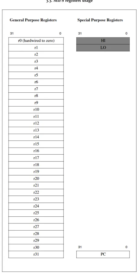
3.3 m i p s r e g i s t e r s u s a g e

MIPS architecture has 32 registers dedicated and there are some conventions to use those registers correctly. Table 3summarizes those registers, and their usage.

Table 3.: MIPS registers

Name Number Use Callee must

preserve?

$zero $0 has constant 0 No

$at $1 register reserved for assembler (temporary) No

$v0 - $v1 $2 - $3 register reserved for returning values of functions,

and expression evaluation No

$a0 - $a3 $4 - $7 registers reserved for function arguments No

$t0 - $t7 $8 - $15 temporary registers No

$s0 - $s7 $16 - $23 saved temporary registers Yes

$t8 - $t9 $24 - $25 temporary registers No

$k0 - $k1 $26 - $27 register reserved for OS kernel N/A

$gp $28 global pointer Yes

$sp $29 stack pointer Yes

$fp $30 frame pointer Yes

$ra $31 return address N/A

Note: N/A (Not applicable)

Table 3is composed of 4 columns:

1. Name displays the identifier of the registers available in MIPS. Those identifiers will be used as operands of MIPS instructions.

(40)

2. Number column defines the number of each register. This number can also be used to refer to the register in an instruction.

3. Use column refers to the meaning/definition of each register.

4. Callee must preserve? column provides information about the volatility of the register (used when a function is called).

Beside those 32 registers, 3 more registers are dedicated to the CPU. And they are known by:

• PC - Program Counter register

• HI - Multiply and Divide register higher result • LO - Multiply and Divide register lower result

PC is the register which holds the address of the instruction that is being executed at the current time; HI and LO registers have different usage according to the instruction that is being executed. In this case, let’s see what context they have:

• when there is a multiply ( mul instruction) operation, the HI and LO registers store the result of integer multiply.

• when there is a multiply-add ( madd instruction) or multiply-subtract ( msub instruc-tion) operation, the HI and LO register store the result of integer multiply-add or multiply-subtract.

• when there is a division ( div instruction) operation, the HI register store the remain-der of the division and the LO register store the quotient of the division operation. • when there is a multiply-accumulate ( instruction) operation, the HI and LO registers

store the accumulated result of the operation. See an overview of the MIPS registers in Figure 3.

(41)

3.3. MIPS registers usage

(42)

3.4 m i p s i n s t r u c t i o n f o r m at s

Instructions, in MIPS, are divided into three types: • R-Type

• I-Type • J-Type

Each instruction is denoted by an unique mnemonic that represents the correspondent low-level machine instruction or operation.

Next sections provide the necessary details.

3.4.1 MIPS R-Type

R-Type instruction refers a register type instruction (it is the most complex type in MIPS). The idea behind that instruction is to operate with registers only.

This type has the following format in MIPS (see Listing 3.1).

1 OP rd , rs , r t

Listing 3.1: R-Type instruction format

In Listing 3.1, the instruction is composed of one mnemonic, denoted by OP, and three operands, denoted by rd (destination register), rs (source register), rt (another source register).

The R-Type instruction format as the following mathematical semantics:

1 rd = r s OP r t

To understand better this instruction, let’s see an example of one R-Type instruction in MIPS (see Listing 3.2).

1 add $t1 , $t1 , $ t 2

Listing 3.2: Example of a R-Type instruction

The instruction shown in Listing 3.2 means that register $t1 shall be added (due to add mnemonic) to register $t2 and their sum (the result) stored in register $t1.

(43)

3.4. MIPS instruction formats OP rd, rs, rt ⇐⇒ rd = rs OP rt ⇓ add $t1, $t1, $t2 ⇐⇒ $t1 = $t1 add $t2 ⇓ $t1 = $t1 + $t2

Table 4defines the bit-structure of a R-Type instruction in a 32-bit machine.

Table 4.: R-Type binary machine code

opcode rs rt rd shift (shamt) funct

6bits 5bits 5bits 5bits 5bits 6bits

Let’s explain each of the columns in Table 4.

• opcode defines the instruction type. For every R-Type instruction, opcode is set to the value 0. The opcode field is 6 bits long (bit 31 to bit 26).

• rs this is the first source register; it is the register where it will load the content of the register to the operation.The rs field is 5 bits long (bit 25 to bit 21).

• rt this is the second source register (same behaviour as rs register). The rt field is 5 bits long (bit 20 to bit 16).

• rd this is the destination register; it is the register where the results of the operation will be stored. The rd field is 5 bits long (bit 15 to bit 11).

• shift amount the amount of bits to shift for shift instructions. The shift field is 5 bits long (bit 10 to bit 6).

• function specify the operation in addition to the opcode field. The function field is 6 bits long (bit 5 to bit 0).

Let’s see an example of a R-Type instruction and its transformation to machine code in Table 5.

(44)

add $t0, $t0, $t1 ⇓ add $8, $8, $9 ⇓ (8)₁₀ = (01000)₂ (9)₁₀ = (01001)₂

add instruction(f unct f ield) = (100000)₂ ⇓

opcode (6bits) rs (5bits) rt (5bits) rd (5bits) shift (shamt) (5bits) funct (6bits)

000000 01000 01001 01000 00000 100000

Table 5.: Transformation of R-Type instruction to machine code

In Table 5, the instruction ’add $t0, $t0, $t1’ will be normalized with the name of the register according to the number associated for the register in MIPS (see Table 3). Then a conversion operation is applied to the two register numbers ( 8 and 9), translating them into their binary number with 5 bits long. Also we give the information for the add instruction, which is set for the MIPS architecture (not predictable).

After that, we complete the table for R-Type instruction according to Table 4 with the informations available and the restriction/rules associated to R-Type instruction in MIPS.

Notice that the opcode field for R-Type instruction are set to the value 0 (according to the explanation in Table 4).

3.4.2 MIPS I-Type

I-Type instruction is a set of instructions which operate with an immediate value and a register value.

Several different Immediate ( I-Type) instructions formats are available. Let’s see those diferents formats for this type in Table 6.

(45)

3.4. MIPS instruction formats 31– 26 25 —- 21 20– 16 15——– 11 10——- 6 5—– 0 opcode rs rt immediate opcode rd offset opcode offset opcode rs rt rd offset

opcode base rt offset function

Table 6.: Distinct I-Type instruction formats

In Table 6, there are 5 differents instruction formats which corresponds to different bit structures as illustrated.

The most frequent MIPS I-Type instruction is the first one, denoted as Imm16 (Imme-diate instruction with 16 bits imme(Imme-diate value), is used for logical operands, arithmetic signed operands, load/store address byte offsets and PC-relative branch signed instruction displacements (see Table 7).

31 — 26 25— 21 20— 16 15—————– 0

opcode rs rt immediate

Table 7.: Immediate (I-Type) Imm16 instruction format

Let’s see examples of Imm16 instruction:

1 addi $t0 , $t0 , 10 / / A r i t h m e t i c o p e r a t i o n 2 o r i $t0 , $t1 , 5 / / L o g i c a l o p e r a t i o n

3 beq $t0 , $t1 , 1 / / C o n d i t i o n a l b r a n c h o p e r a t i o n 4 lw $t0 , a r r a y 1 ( $ t 0 ) / / Data t r a n s f e r o p e r a t i o n

The second instruction, denoted as Immediate Off21 instruction (Immediate instruction with 21bits offset), is used for comparing a register against zero and branch (offset field is larger than the usual 16-bit field (immediate field of the first instruction from the table above)). See Table 8.

31— 26 25— 21 20——————— 0

opcode rd offset

Table 8.: Immediate (I-Type) Off21 instruction format

The third instruction, denoted as Immediate Off26 instruction (Immediate instruction with 26 bits offset), is used for PC-relative branches with very large displacements (uncon-ditional branches (BC mnemonic instruction) & branch-and-link (BALC mnemonic instruc-tion) with a 26-bit offset,). See Table 9.

(46)

31— 26 25———————————— 0

opcode offset

The fourth instruction, denoted as Immediate Off11 instruction (Immediate instruction with 11 bits offset), is used for the newest encodings of coprocessor 2 load and store instruc-tions (LWC2, SWC2, LDC2, SWC2). See Table 10.

31— 26 25—– 21 20——— 16 15 ———– 11 10 ——————- 0

opcode rs rt rd offset

Finally, the last one (fifth instruction), denoted as Immediate Off9 instruction (Immediate instruction with 9 bits offset), is used for SPECIAL3 instructions such as EVA memory access ( LBE mnemonic). Also this is primarly used for instruction encodings that have been moved, such as LL menmonic and SC mnemonic instruction. See Table 11.

31 — 26 25—– 21 20——— 16 15—————— 7 6 5——————- 0

opcode base rt offset 0 function

Table 11.: Immediate (I-type) Off9 instruction format

Notice that, for the project related to the thesis, only the first instruction type (Immediate (I-Type) Imm16 instruction format) was used. The other instruction formats are not really important for this project.

3.4.3 MIPS J-Type

J-Type instructions are instructions which jump to a certain address. Let’s see his format in Table 12.

31— 26 25—————————————————————– 0

opcode address

Table 12.: J-Type instruction format

In Table 12, 6 bits are associated to the opcode field and 26 bits for the address field. But notice that in MIPS, addresses are 32 bits long.

For solving that, MIPS use a technique which leads to shift the address left by 2 bits and then combine 4 bits with the 4 high-order bits of the PC in front of the address.

(47)

3.5. MIPS assembly language

2 j r $ r a / / Jump r e g i s t e r i n s t r u c t i o n

3 j w r i t e l n / / Jump i n s t r u c t i o n

Listing 3.3: Examples of J-Type instruction

In Listing 3.3, we see three different types of jump instruction. The first one example, is a jal instruction and it means ’jump and link’ in an extensive way. Basically, it jump to the branch written in front of the jal nomenclature and stores the return address (instantly) to the return address register ($ra; $31). In this way, the programmer don’t need to use some instructions for saving the return address and continue the flow of the execution code.

The second example, is a jr instruction and it means ’jump to an address stored in a register’. Notice that registers are available in the MIPS architecture.

The third and last example is a j instruction and this is a ’jump instruction’. Summing it up, it jumps to the branch written in front of the letter j, which is in this case writeln.

3.5 m i p s a s s e m b ly l a n g ua g e

MIPS language is divided into 2 parts (Data and Text parts).

3.5.1 MIPS data declarations

This section is used for declaring variable names used in the program. Variables declared are allocated in the main memory (RAM) and must be identified with a particular nomen-clature denoted as .data. It is used for declaring global variables, principally.

Then comes the part when the variable names are declared. Let’s see the format for declaring a variable name in Listing 3.4.

1 name : s t o r a g e t y p e value ( s )

Listing 3.4: Syntax format of data declarations in MIPS

In Listing 3.4, the name field refers to the name of the variable. The storage type refers to the type of the variable that can be:

• .ascii store a string in memory without a null terminator. • .asciiz store a string in memory with the null terminator. • .byte store ’n’ bytes contiguously in memory.

• .halfword store ’n’ 16-bit halfwords contiguously in memory. • .word store ’n’ 32-bit words contiguously in memory.

(48)

• .space store a certain number of bytes of space in memory. Last, the value(s) field refers to the value of the type associated.

Let’s see some example for declaring some variables in MIPS in Listing 3.5.

1 . data # T e l l s a s s e m b l e r we ’ r e i n t h e d a t a s e g m e n t

2 v a l : . word 1 0

3 s t r : . a s c i i ” Hello , world ”

4 num : . byte 0x01 , 0 x02

5 a r r : . space 100

Listing 3.5: Examples for declaring variables in MIPS

In Listing 3.5, there are 4 different types under the data section.

The variable val contains the value ’10’ and the size of the variable is 32 bits.

The variable str contains the string ’Hello World’ and the size of the variable is the same size as the string.

The variable num stores the listed value(s) (which appears after the .byte nomenclature) as 8 bit bytes. In this example, it will be ’0x00000201’.

The variable arr reserves the next specified number of bytes in the memory, which will be 100 bytes reserved for that variable.

3.5.2 MIPS text declarations

This section contains the program code and follows a specific syntax starting with the keyword .text.

As all programming languages, there is a starting point in the code that must be desig-nated as main:. Each of the assembly language statements in MIPS (written after the main: field) are executed sequentially (excepted loop and conditional statements).

1 . t e x t

2 main :

3 l i $t0 , 5

4 l i $t1 , 10

5 mul $t0 , $t0 , $ t 1

Listing 3.6: Example of Text declarations in MIPS

In Listing 3.6, we see the .text which begins the code of the program and the main: which shows where the code execution must start.

(49)

3.5. MIPS assembly language

In this case, it will load two numbers in different registers and multiply them (see Section 3.6to understand those instructions).

Notice that the code will execute sequentially.

Also, in the text part beside of the code execution flow, we can write the name of branches for executing some jump instructions. This means that every jump instruction with a name associated, will see if that name is under the text part. Like that when a jump instruction is available it can jump to the name associated.

And for this purpose, we need to add some context to the MIPS jump instruction code and understand it better.

In this case, we need to replicate the same syntax as the main: field but with the correct name of the condition or the loop (also inside of the text declarations parts). Like that, MIPS knows where it must jump for the next instruction. Let’s look an example in Listing 3.7. 1 . data 2 . t e x t 3 main : 4 l i $t0 , 5 5 l i $t1 , 5 6 mul $t0 , $t0 , $ t 1 7 j a l j u m p c o n d i t i o n # n e e d s t o jump t o t h e f i e l d j u m p c o n d i t i o n 8 l i $t0 , 4 9 l i $v0 , 10 10 s y s c a l l

11 j u m p c o n d i t i o n : # s y n t a x f o r jump and c o n d i t i o n a l i n s t r u c t i o n i n mips

12 l i $t1 , 5

13 j r $ r a

Listing 3.7: Example of a loop declaration in MIPS

As we can see in Listing 3.7, we have a jal instruction available and a name associated next to the instruction. This name must be included under the .text section, because the name is the name of the branch from where the jump instruction will jump. If the name isn’t in the MIPS assembly code, then the program cannot execute the assembly code. But in the example case, we can see that the name is available below as jump condition:. So this means that the jal instruction will jump to that line and continue the code execution flow there.

Also, in MIPS, there is the possibility to include inline comments in the code using the symbol # on a line (see Listing 3.8).

(50)

Listing 3.8: Example of a comment in MIPS

Let’s see the template for a MIPS assembly language program in Listing 3.9.

1 # Comment g i v i n g name o f program and d e s c r i p t i o n o f f u n c t i o n 2 # T e m p l a t e . s

3 # Bare−b o n e s o u t l i n e o f MIPS a s s e m b l y l a n g u a g e program 4 5 . data # v a r i a b l e d e c l a r a t i o n s f o l l o w t h i s l i n e 6 # . . . 7 8 . t e x t # i n s t r u c t i o n s f o l l o w t h i s l i n e 9 10 main : # i n d i c a t e s s t a r t o f c o d e ( f i r s t i n s t r u c t i o n t o e x e c u t e ) 11 # . . .

Listing 3.9: Template of a MIPS assembly language

3.6 m i p s i n s t r u c t i o n s

MIPS has 6 type of instructions : • instructions for data transfer

• instructions for arithmetic operations • instructions for logical operations • instructions for bitwise shift • instructions for conditional branch • instructions for unconditional branch

Let’s see some examples of those instructions and their meanings.

Table 13.: Example of Data transfer instruction in MIPS

Name Instruction

Syntax Meaning Format Opcode Funct

Store word sw $t,C($s) Memory[ $s + C] = $t I 0x2B N/A

Load word lw $t,C($s) $t = Memory[$s + C] I 0x23 N/A

(51)

3.6. MIPS instructions

Table 14.: Example of Arithmetic instruction in MIPS

Syntax Meaning Type Opcode Funct

Add add $d, $s, $t $d = $s + $t R 0x0 0x20

Add

immediate addi $t, $s, C $t = $s + C (signed) I 0x8 N/A

Subtract sub $d, $s, $t $d = $s - $t R 0x0 0x22 Move move $t0, $t1 $t0 = $t1 R 0x0 0x21 Multiply mul $s, $t, $d $s = $t * $d LO = $t * $d (upper 32bits) HI = $t * $d (lower 32bits) R 0x0 0x19 Divide div $s, $t, $d $s = $t / $d LO = $t / $d HI = $t % $d R 0x0 0x1A

Table 15.: Example of Logical instruction in MIPS

Set on less than slt $d,$s,$t $d = ($s <$t) R 0x0 0x2A

Or or $d,$s,$t $d = $sk$t R 0x0 0x25

And and $d,$s,$t $d = $s & $t R 0x0 0x24

Set on less than unsigned sltu $d,$s,$t $d = ($s <$t) R 0x0 0x2B

Exclusive or immediate xori $d,$s,C $d = $s ˆC I 0xE N/A

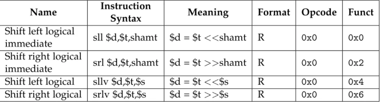
Table 16.: Example of Bitwise Shift instruction in MIPS

Shift left logical

immediate sll $d,$t,shamt $d = $t <<shamt R 0x0 0x0

Shift right logical

immediate srl $d,$t,shamt $d = $t >>shamt R 0x0 0x2

Shift left logical sllv $d,$t,$s $d = $t <<$s R 0x0 0x4

Shift right logical srlv $d,$t,$s $d = $t >>$s R 0x0 0x6

Some explanation must be provided for understanding the tables shown previously: • PC means Program Counter.

• target means the name of the target (used for jump instructions). • C means constants.

• 0x.. means a hexadecimal format number. • N/A means Not Applicable.

(52)

Table 17.: Example of Conditional Branch instruction in MIPS

Branch if equal

zero beqz $s, jump

if($s==0) go to

jump address I 0x4 N/A

Branch on not

equal bne $s, $t, C

if ($s != $t) go to

PC+4+4*C I 0x5 N/A

Branch on equal beq $s, $t,C if ($s == $t) go to

PC+4+4*C I 0x4 N/A

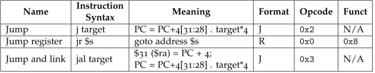
Table 18.: Example of Unconditional Branch instruction in MIPS

Jump j target PC = PC+4[31:28] . target*4 J 0x2 N/A

Jump register jr $s goto address $s R 0x0 0x8

Jump and link jal target $31 ($ra) = PC + 4;

PC = PC+4[31:28] . target*4 J 0x3 N/A

• shamt means the number to shift (used in shift instructions).

Note that the Format, Opcode and Funct are the information of each field for each format instruction as explained in Section 3.4.

Beside those instructions, some other instructions are sequences of instructions and they are called as pseudo instructions (see in Table 19).

Table 19.: Example of Pseudo Instructions in MIPS

Syntax Real instruction translation Meaning

Move move $d, $s add $d, $s, $zero $d=$s

Load Address la $d, LabelAddr lui $d, LabelAddr[31:16]

ori $d, $d, LabelAddr[15:0] $d = Label Address Multiplies and

returns only first 32bits

mul $d, $s, $t mult $s, $t

mflo $d $d = $s * $t

Divides and

returns quotient div $d, $s, $t

div $s, $t

mflo $d $d = $s / $t

Branch if equal

to zero beqz $s, Label beq $s, $zero, Label if ($s==0) PC=Label

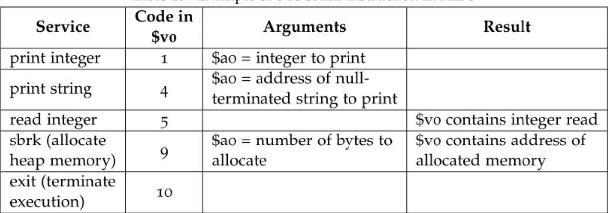
Additionally, MIPS includes a number of system services for input and output interaction, denoted as SYSCALL. Let’s see an example of those services in Table 20.