Distributed Algorithms for Target Localization in Wireless Sensor Networks Using Hybrid Measurements

(1)

David José Marques Vicente

Licenciado em Ciências da Engenharia Electrotécnica e de Computadores

Distributed Algorithms for Target Localization in

Wireless Sensor Networks Using Hybrid

Measurements

Dissertação para obtenção do Grau de Mestre em Engenharia Electrotécnica e de Computadores

Orientador: Marko Beko, Investigador Auxiliar, UNINOVA

Co-orientador: Rui Miguel Henriques Dias Morgado Dinis,

Professor Associado com Agregação, FCT-NOVA

Júri

Presidente: Rodolfo Alexandre Duarte Oliveira

(2)

(3)

Distributed Algorithms for Target Localization in Wireless Sensor Networks Using Hybrid Measurements

A Faculdade de Ciências e Tecnologia e a Universidade NOVA de Lisboa têm o direito, perpétuo e sem limites geográficos, de arquivar e publicar esta dissertação através de exemplares impressos reproduzidos em papel ou de forma digital, ou por qualquer outro meio conhecido ou que venha a ser inventado, e de a divulgar através de repositórios científicos e de admitir a sua cópia e distribuição com objetivos educacionais ou de inves-tigação, não comerciais, desde que seja dado crédito ao autor e editor.

Este documento foi gerado utilizando o processador (pdf)LA_{TEX, com base no template “novathesis” [1] desenvolvido no Dep. Informática da FCT-NOVA [2].}

(4)

(5)

(6)

(7)

A c k n o w l e d g e m e n t s

Gostaria de agradecer ao meu orientador, o Professor Marko Beko. Pela disponibilidade e paciência ao longo de todo o percurso que levou à escrita desta dissertação. Pelo à-vontade que demonstrou logo desde o início. E por manter um espírito positivo mesmo quando as situações não corriam da melhor forma.

Quero também agradecer ao meu colega Slavisa Tomic. Por toda a preciosa ajuda e tempo que disponibilizou, e pelas explicações esclarecedoras.

Um obrigado aos meus amigos, com quem tive a oportunidade de trabalhar várias vezes ao longo do curso: André Pontes, Afonso Ferreira, Diogo Basílio, Emanuel Sequeira, Guilherme Gaspar, Ivo Bernardino, João Matias, Ricardo Lima, Tiago Aleixo, Tiago Pina. Mais recentemente, Gonçalo Leandro e Pedro Mateus. Em especial, um obrigado ao Carlos Filipe, que me deucarryem várias práticas de electrónica.

Quero também agradecer aos restantes membros do auto-intitulado grupo doSAL, simplesmente por estarem presentes.

Aos meus colegas e amigos que tive o prazer de conhecer no decorrer deste percurso e com quem também tive a oportunidade de trabalhar, um obrigado, Flávio Jacinto, João Eusébio Henriques, Ana Filipa Sebastião.

Um obrigado à minha, felizmente, muito numerosa família que sempre me deu força e acreditou em mim. Todos os primos, primas, tios, tias, avó, avô, que de uma forma ou de outra contribuíram para o meu sucesso.

Um obrigado especial aos meus pais, António e Filomena, que todos os dias às 9:00h já estão a "lutar" para que eu e o meu irmão possamos estudar. Que sempre acreditaram e se esforçam incondicionalmente. Ao meu irmão, Henrique, que várias vezes cozinhou para mim quando mais uma hora de estudo fazia toda a diferença.

Quero também deixar um obrigado ao Carlos, à Isabel e ao João. Que me acolheram nestes últimos anos e me recebem todos os dias em sua casa.

(8)

(9)

A b s t r a c t

This dissertation addresses the target localization problem in wireless sensor networks (WSNs). WSNs is now a widely applicable technology which can have numerous practical applications and off_{er the possibility to improve people’s lives. A required feature to} many functions of a WSN, is the ability to indicate where the data reported by each sensor was measured. For this reason, locating each sensor node in a WSN is an essential issue that should be considered.

In this dissertation, a performance analysis of two recently proposed distributed local-ization algorithms for cooperative 3-D wireless sensor networks (WSNs) is presented. The tested algorithms rely on distance and angle measurements obtained from received signal strength (RSS) and angle-of-arrival (AoA) information, respectively. The measurements are then used to derive a convex estimator, based on second-order cone programming (SOCP) relaxation techniques, and a non-convex one that can be formulated as a gener-alized trust region sub-problem (GTRS). Both estimators have shown excellent perfor-mance assuming a static network scenario, giving accurate location estimates in addition to converging in few iterations.

The results obtained in this dissertation confirm the novel algorithms’ performance and accuracy. Additionally, a change to the algorithms is proposed, allowing the study of a more realistic and challenging scenario where diff_{erent probabilities of communication} failure between neighbor nodes at the broadcast phase are considered. Computational simulations performed in the scope of this dissertation, show that the algorithms’ perfor-mance holds for high probability of communication failure and that convergence is still achieved in a reasonable number of iterations.

(10)

(11)

R e s u m o

Esta dissertação aborda o problema da localização de sensores alvo em redes de sensores sem fios. A tecnologia das redes de sensores sem fios é amplamente aplicável actualmente, tendo numerosas aplicações práticas e a capacidade de melhorar a vida das pessoas. Uma propriedade necessária a muitas funções neste tipo de redes, é a capacidade para indicar o local onde foram medidos os dados reportados por cada sensor. Desta forma, localizar cada sensor, numa rede de sensores sem fios, torna-se uma questão essencial a ser considerada.

Nesta dissertação, é apresentada uma análise de desempenho de dois algoritmos de localização recentemente propostos para redes de sensores sem fios cooperativas e em 3 dimensões. Os algoritmos testados fazem uso de medições de distâncias e ângulos, obtidos através da potência do sinal recebido e do ângulo de chegada do sinal, respectivamente. As medições são posteriormente usadas para deduzir um estimador convexo, baseado em técnicas para relaxar problemas através de programação cónica de segunda ordem, e um estimador não convexo, que pode ser formulado como um sub-problema generalizado de região de confiança. Ambos os estimadores demonstram um excelente desempenho, assumindo um cenário em que a rede é estática, fornecendo estimativas de localização com precisão para além de convergirem em poucas iterações.

Os resultados obtidos nesta dissertação confirmam o desempenho e precisão dos dois algoritmos recentemente propostos. Adicionalmente, foi proposta uma alteração aos algo-ritmos que permite estudar um cenário mais realista e desafiante, onde são consideradas diferentes probabilidades de falha de comunicação entre sensores vizinhos, durante a fase de difusão. As simulações computacionais levadas a cabo no âmbito desta disserta-ção, demonstram que o desempenho dos algoritmos se mantém para cenários com alta probabilidade de falhas de comunicação, e que a convergência continua a ser alcançável num número razoável de iterações.

(12)

(13)

C o n t e n t s

List of Figures xv

List of Tables xvii

Glossary xix

Acronyms xxi

Notation xxiii

1 Introduction 1

1.1 Motivation . . . 1

1.2 Objectives and Contributions . . . 3

1.3 Organization . . . 3

2 State of the Art 5 2.1 Introduction . . . 5

2.2 Classification of Localization Schemes . . . 6

2.2.1 Computational Organization . . . 6

2.2.2 Anchor-based and Anchor-free . . . 7

2.2.3 Range-based and Range-free . . . 8

2.3 Range Estimation Methods . . . 9

2.3.1 Received Signal Strength . . . 9

2.3.2 Time of Arrival . . . 10

2.3.3 Time Diff_{erence of Arrival} _{. . . .} ₁₂

2.3.4 Angle of Arrival . . . 13

2.4 Range Combining Techniques . . . 13

2.4.1 Geometric Approaches . . . 14

2.4.2 Optimization Based Approaches . . . 16

(14)

CO N T E N T S

3 Hybrid Distributed Algorithms 21

3.1 Introduction . . . 21

3.2 Problem Statement . . . 22

3.2.1 Assumptions . . . 24

3.3 Distributed Localization . . . 25

3.3.1 KnownP0i’s . . . 26

3.3.2 UnknownP0i’s . . . 30

3.4 Link Failure Scenario . . . 31

3.5 Complexity Analysis . . . 32

4 Computational experiments 35 4.1 Introduction . . . 35

4.2 Framework . . . 35

4.3 Results . . . 36

5 Conclusions and Future Work 43 5.1 Introduction . . . 43

5.2 Conclusions . . . 43

5.3 Future Work . . . 44

Bibliography 47

A Article Submitted toInternational Young Engineers Forum on Electrical and

Computer Engineering, May 2017 55

(15)

L i s t o f F i g u r e s

2.1 Overview of distance and connectivity methods . . . 8

2.2 Eff_{ects of errors in RSS-based range measurements versus distance.} _{. . . . .} ₁₀

2.3 Illustration of diff_{erent ToA methods} _{. . . .} ₁₁

2.4 Illustration of TDoA. . . 12

2.5 Eff_{ects of errors in AoA measurements versus distance.}_{. . . .} ₁₄

2.6 Illustration of trilateration. . . 15

2.7 Illustration of the steps required to perform triangulation. . . 15

2.8 Illustration of the steps required to perform hyperbolic positioning. . . 16

2.9 Use of an optimization method to combine noisy measurements in overdeter-mined systems. . . 18

2.10 Use of optimization methods to combine noisy hybrid (distance and angle) measurements. . . 19

3.1 Illustration of a target’s relative distance and angles to an anchor.. . . 23

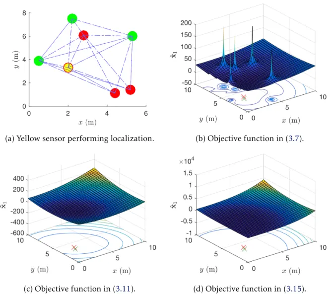
3.2 (a) Illustration of a sensor (in yellow) performing self-localization in a 2-D WSN (green dots are anchors, red dots are targets). RSS and AoA measure-ments are used. Figures (b) (c) and (d) show the respective objective functions in (3.7), (3.11) and (3.15) (minus the elevation angle terms) versusx(m) and y(m). The yellow sensor’s real coordinates are projected, in the contours part of the plot, as a green cross in (b) (c) (d), each objective function’s minimum is projected as a red cross. . . 29

4.1 A randomly generated WSN withN= 20,M= 50,R= 6.5 andd0= 1. . . 36

4.2 NRMSE versus t comparison, whenN = 20,M = 50,R= 6.5 m,σnij = 3 dB, σmij = 6 deg, σvij = 6 deg,γij ∈U[2.7,3.3],γ = 3, B= 20 m,P0i ∈U[−12,−8] dBm,d0= 1 m,Mc= 500. . . 37

4.3 NRMSE versus t comparison, whenN = 30,M = 50,R= 6.5 m,σnij = 3 dB, σ_m_ij = 6 deg, σ_v_ij = 6 deg,γ_ij ∈U[2.7,3.3],γ = 3, B= 20 m,P0i ∈U[−12,−8] dBm,d0= 1 m,Mc= 500. . . 38

(16)

L i s t o f F i g u r e s

4.5 NRMSE versusσnij (dB) comparison, whenN= 20,M= 50,R= 6.5 m,σmij = 1

deg,σvij = 1 deg,γij∈U[2.7,3.3],γ = 3,Tmax= 30,B= 20 m,P0i∈U[−12,−8]

dBm,d0= 1 m,Mc= 500. . . 39 4.6 NRMSE versusσ_m_ij(deg) comparison, whenN= 20,M= 50,R= 6.5 m,σ_n_ij = 1

dB,σvij = 1 deg,γij ∈U[2.7,3.3],γ = 3,Tmax= 30, B= 20 m,P0i∈U[−12,−8]

dBm,d0= 1 m,Mc= 500. . . 40 4.7 NRMSE versusσ_v_ij (deg) comparison, whenN= 20,M= 50,R= 6.5 m,σ_n_ij = 1

dB,σmij = 1 deg,γij∈U[2.7,3.3],γ = 3,Tmax= 30,B= 20 m,P0i ∈U[−12,−8]

dBm,d0= 1 m,Mc= 500. . . 41 4.8 NRMSE versus t comparison for “SOCP”, when N = 20, M = 50, R = 6.5

m, σnij = 3 dB, σmij = 6 deg, σvij = 6 deg, γij ∈U[2.7,3.3], γ = 3, B= 20 m,

P0i∈U[−12,−8] dBm,d0= 1 m,Mc= 500, varyingPf. . . 41 4.9 NRMSE versust comparison for “SR-WLS”, whenN = 20, M = 50, R= 6.5

P0i∈U[−12,−8] dBm,d0= 1 m,Mc= 500, varyingPf. . . 42 4.10 NRMSE versus t comparison for “uSOCP”, when N = 20, M = 50, R= 6.5

P0i∈U[−12,−8] dBm,d0= 1 m,Mc= 500, varyingPf. . . 42

(17)

L i s t o f Ta b l e s

2.1 Path Loss Exponent values for diff_{erent environments [55]} _{. . . .} ₁₀

(18)

(19)

G l o s s a r y

anchors Sensor nodes whose locations are known from the very start. The infor-mation is either obtained by manual configuration during deployment, or by external means such as GPS. A reference node .

sensor A device which is connected, via a RF communication medium, to the other devices in the network. Throughout this document the terms ’sensor’, ’sensor node’ and ’node’ all refer to the same thing and are used interchangeably .

(20)

(21)

A c r o n y m s

AoA angle of arrival.

BS base station.

GPS global positioning system.

GTRS generalized trust region sub-problem.

IoT Internet of Things.

LAN local area network.

LoS line-of-sight.

LS least squares.

Mc Monte Carlo.

MLE maximum likelihood estimate.

NLoS non-line-of-sight.

PDF probability density function.

PLE path loss exponent.

RF radio frequency.

(22)

AC R O N Y M S

RSSI received signal strength indicator.

SDP semidefinite programming.

SOCP second-order cone programming.

SR-WLS squared-range weighted least squares.

TDoA time diff_{erence of arrival.}

ToA time of arrival.

WSNs wireless sensor networks.

(23)

N o t a t i o n

For reference purposes, some of the most common symbols used throughout the disser-tation are listed below. Upper-case bold type, lower-case bold type and regular type are used for matrices, vectors and scalars, respectively.

R _{the set of real numbers}

Rn _{n-dimensional real vectors}

Rm×n _m_×_n_{real matrices}

AT the transpose ofA

A−1 the inverse ofA

I_n then×nidentity matrix

0_m×n them×nmatrix of all zero entries

1_n then-dimensional column vector with all entries equal to one

diag(x) the square diagonal matrix with the elements of vectorxas its main diagonal, and zero elements outside the main diagonal

kxk the Euclidean norm of vectorx;_kxk=√xT_x_{, where}_x_∈Rn_{is a}

column vector

p(_·) probability density function

N(µ,Σ₎ _{real-valued Gaussian distribution with mean vector}_µ_{and covariance} matrixΣ

∼ distributed according to

≈ approximately equal to

(24)

(25)

C

h

a

p

t

e

r

1

I n t r o d u c t i o n

1.1 Motivation

Wireless sensor networks (WSNs)have gone from just a vision to a widely applicable tech-nology in merely three decades. Small, low-cost and low-power devices equipped with sensor(s), a microprocessor and a transceiver, monitor physical phenomena in an area of interest, communicating through wireless links. The observed physical or environmental conditions can be light, sound, temperature, vibration, pressure or even vital signs, to name a few [1,15].

Such characteristics grant the possibility for WSNs to have numerous applications in areas like environmental monitoring, military and home domain. For example, farmers can use this type of technology to monitor the soil conditions, industrial bodies may use it to track greenhouse emissions, and it may provide battlefield advantage to the military thanks to its rapid deployment and self organization characteristics. Also pushing the research and development of WSNs is the currently trending concept calledInternet of Things (IoT)[72], "a world-wide network of interconnected objects uniquely addressable, based on standard communication protocols" [30]. This vision of IoT is driving the usage of sensors in applications such as smart homes and intelligent transportation systems, acting as a bridge between the physical and digital world [3].

(26)

C H A P T E R 1 . I N T R O D U C T I O N

coordinates of each sensor node, as manual localization of every node would be prone to human error and unfeasible in a realistic amount of time. A problem arises however, as sensor nodes should be able to indicate where the gathered data was recorded, since a set of measurements without location information is only useful to compute simple statistics such as the average of said measurements.

Localization of sensor nodes in a WSN is required in many practical applications, namely: event detection (fires, floods) [62], monitoring (health care, industrial, agricul-tural, environmental) [16,38,56], exploration (underground, deep water, outer space) [23], and surveillance (intrusion detection) [28]. Furthermore, there are routing protocols that require the nodes’ locations in order to make multi-hop communication decisions and energy-effi_{cient routing [}₂_, ₉_{]. By knowing each node’s location it is also possible to} evaluate the node density and coverage of the interest area. Lastly, localization enables context-awareness, identification and correlation of gathered data, allowing statistics to be computed in terms of spatial sampling rather than the count of sensor readings [10].

All of above mentioned points make the localization of each node after the deployment phase a high priority issue. Therefore, localization techniques should be used to estimate each node’s location so that the network is able to organize itself.

The most obvious solution to this matter would be equipping each node with aglobal positioning system (GPS)receiver, rendering the localization problem trivial (in favorable conditions). This method, however, is unsuitable for WSNs considering the constraints to which the devices are subject like low production cost, low complexity and low power con-sumption [49]. Furthermore, GPS requiresline-of-sight (LoS)signal propagation between the satellites and the receiver resulting in possible obstruction by trees, tall buildings, etc. The system is also unreliable in specific environments like indoors and underground tunnels, as the signal cannot penetrate walls and soil very well [34]. Consequently, being able to perform localization using diff_{erent approaches should be considered.}

Another, more effi_{cient, approach to localization in WSNs is to establish the position of} sensor nodes whose location is unknown (targets), given some information about a sparse number of reference sensors (anchors), possibly equipped with GPS receivers, in addition to measured distances/angles between any pair of nodes. To obtain such measurements, one can exploit diff_{erent characteristics of the}_{radio frequency (RF)}_{signals used by the} nodes to communicate [49].

In summary, knowing the exact location of each sensor node is of utmost importance, making localization techniques a key factor in WSNs and motivating the development of effi_{cient localization schemes.}

(27)

1 . 2 . O B J E C T I V E S A N D CO N T R I B U T I O N S

1.2 Objectives and Contributions

The goal of this dissertation is to present an overview of the localization estimation in WSNs theme and to study two range-based, distributed and cooperative algorithms for target localization in WSNs proposed in [68]. The main contributions are:

• An implementation of two distributed localization algorithms, taking advantage of combined RSS/AoA measurements in a cooperative 3-D WSN, based on:

– Second-order cone programming (SOCP)relaxation;

– Generalized trust region sub-problem (GTRS)framework.

• An implementation of the algorithm based on SOCP, generalized for diff_{erent and} unknown transmit powers.

• A proposed change to the distributed localization algorithms, so that failure be-tween neighbor nodes at the broadcast phase is considered.

• A computational experiment based on theMonte Carlo (Mc)method, providing a probabilistic interpretation of the algorithms’ performances.

• A comparative analysis on the performance of the algorithms.

• A study of the algorithms’ behavior in view of diff_{erent probabilities of} communi-cation failure.

The work conducted in this dissertation resulted in the following submission:

D. Vicente, S. Tomic, M. Beko, and R. Dinis, "Performance Analysis of a Dis-tributed Algorithm for Target Localization in Wireless Sensor Networks Using Hy-brid Measurements in a Connection Failure Scenario", Submitted toInternational Young Engineers Forum on Electrical and Computer Engineering, May 2017.

1.3 Organization

The dissertation structure is briefly organized as follows:

(28)

C H A P T E R 1 . I N T R O D U C T I O N

Chapter3 presents the general mathematical formulation of the localization problem, followed by the introduction of some of the techniques explained in the previous chapter. The studied algorithms are derived and then presented in the form of pseudo-code. Lastly, the contribution of this work is also presented.

Chapter4 consists of the information relative to the carried computational experiments. Each experimental environment is explained and the respective results are dis-played in the form of comparative plots.

Chapter5 draws the conclusions and suggests future work directions.

AppendixA presents the submitted article, which is based on the contribution made in this work.

(29)

C

h

a

p

t

e

r

2

S t a t e o f t h e A rt

2.1 Introduction

The idea of wireless positioning was initially conceived for cellular networks. In this dissertation we limit our discussion to sensor localization in WSNs. However, it is worth noting that, in practice, a base station (BS)or an access point in a local area network (LAN)can be considered as an anchor, while other devices such as cell phones, laptops, tags, etc., can be considered as targets. [59]

The goal of localization can be stated as: for each node with an unknown position, find and assign its geographic coordinates in the area of interest. For most WSNs applications, sensor data should be accompanied with an indication of the physical location where the data was recorded. Even if the accessible knowledge about positions of nodes is only approximate, there are many other tasks done in a WSN that benefit from it, namely: network services, location-based routing, data aggregation, etc [10].

While localization is a required feature to many functions in a WSN, it is not the real purpose of it. Therefore, localization should cost as little as possible in terms of network resources while still producing satisfactory results. In other words, the power cost, hardware cost, and deployment cost of nodes should be minimized [4].

It is possible to classify location discovery algorithms based on several criteria and used techniques. These algorithms should work with inexpensive off_{-the-shelf hardware,} have minimal energy requirements, scale to large networks, and also achieve good ac-curacy independently of the surrounding environment, giving the solution in a short amount of time [46].

(30)

C H A P T E R 2 . S TAT E O F T H E A R T

Next, the contrast amidst collaborative and non-collaborative networks is detailed. Then, two ways of obtaining distance estimates between sensors are explained, followed by a discussion about the main ranging techniques used in range-based localization schemes. Finally, the most basic range-combining techniques are introduced, in addition to dedi-cating some attention to schemes based on hybrid measurements.

2.2 Classification of Localization Schemes

Localization schemes can be classified according to many criteria that reflect design choices and structural features. The distinctions are made generally when addressing known challenges in localization (computing organization, measurement techniques, ex-istence of reference/anchor nodes, node mobility, position estimation accuracy, etc.). The rest of this section describes in more detail the most relevant criteria in the context of this dissertation.

2.2.1 Computational Organization

A typical issue in WSNs is the computational constraints to which this type of networks are subject. In order to maintain the network’s overall cost low, sensor nodes are limited in power, computational capacities, and memory [1]. There are two approaches to address how computation is performed in the network [31], both are described next:

Centralized This approach assumes the existence of a sink node which acts as a central processor. Each sensor node sends the measured information (distance, orientation, connectivity) to the sink. This central node gathers all the measurements and solves the localization problem, forwarding the result back to the sensor nodes afterwards.

Distributed In this approach, computation is distributed between every sensor node. Targets usually use information from neighbor and anchor nodes to determine their position.

The centralized approach off_{ers e}ffi_{cient processing and addresses the computational} constraints present in low-cost sensor nodes. However, this way of tackling the problem suggests communication overhead, as each node has to make more transmissions in order to relay measured information, resulting in a higher battery consumption. Furthermore, this model introduces a single point of failure in the network, meaning that the entire localization process fails in case there is a sink node failure [50].

For large-scale and highly-dense networks, applying a distributed model becomes a preferable solution [17]. This approach requires higher processing capabilities from each sensor node but decreases communication overhead compared to the former model. Nonetheless, distributed algorithms are executed iteratively, which raises the energy consumption of the processing tasks and makes them prone to error propagation. The

(31)

2 . 2 . C L A S S I F I CAT I O N O F LO CA L I Z AT I O N S C H E M E S

work in [49] states that, when the necessary number of iterations required for conver-gence is lower than the average number of hops to the central processor, the distributed approach is likely to be more energy-effi_{cient. Examples of centralized algorithms are} the MDS-MAP [60] and the semidefinite programming (SDP)based algorithm in [18]. Some exemplars of distribuited algorithms are the APS [43], the APIT [27], the bounding box [61] and the gradient [5].

2.2.2 Anchor-based and Anchor-free

It is possible to classify localization schemes regarding its use of anchor nodes. Anchors are a set of nodes that are aware of their coordinatesa priori, either by using some external system like GPS or through manual configuration during deployment.

The goal of anchor-based schemes is to provide partial information of the entire net-work to a localization algorithm. This way, the algorithm can extrapolate the coordinates of non-anchors based on this information [58]. With anchor-based schemes the network’s coordinate system can be aligned with a global coordinate system, making it possible to obtain absolute coordinates like latitude, longitude and altitude for each target. Still, GPS receivers are expensive and equipping anchors with them in high scale networks might not be viable. Plus, GPS requires LoS communication which typically does not work indoors as the signal cannot penetrate walls reliably and can be obstructed by envi-ronmental obstacles [34]. The alternative of pre-programming nodes with their locations is impractical, for the same scalability reasons, or even impossible, depending on the interest area’s accessibility or the method of deployment. Another downside is that accu-racy relies heavily on the number of anchor nodes and their geographic placement in the network. It has been found that localization accuracy improves if anchors are deployed in a convex hull around the network, but additional targets at centre of it is also benefi-cial [4]. Yet, the big advantage of using anchor nodes is greatly simplifying the task of obtaining coordinates for the unknown location nodes.

Anchor-free schemes, as the name implies, do not rely ona priorilocalization infor-mation from a set of nodes in order to make assumptions about the remaining nodes’s positions [41,53]. This type of localization scheme picks a set of reference nodes to estab-lish a coordinate system, and estimates relative positions to it for the other nodes. One obvious advantage of not requiring anchors is the possibility of performing localization in environments where it is impossible to get GPS signal. However, if at least one of the reference nodes moves, positions have to be recomputed for all the nodes, even if no other nodes have moved [74].

Target Collaboration

(32)

nodes can not communicate with anchors. Still, targets need to be within communication range of anchors in order to perform range measurements that are needed for localization estimation. However, in this conditions their ability to perform self-location is limited if not impossible. Collaboration between target nodes is the mechanism used to face this issue. A collaborative localization scheme allows target nodes to communicate with either anchors or targets, improving localization accuracy and coverage [76].

2.2.3 Range-based and Range-free

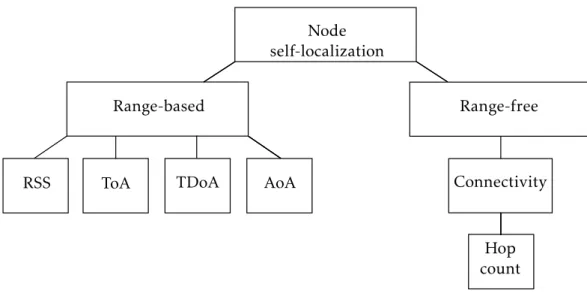
Localization schemes are in general classified as range-based or range-free with regard to the mechanisms used to estimate inter-node distances. Range-based schemes use absolute pairwise distance and/or orientation measurements for coordinates computation. Range-free schemes, on the other side, rely solely on connectivity information to locate the sensors. An overview of the two can be seen in Figure2.1.

Range-based Range-free

AoA

ToA TDoA

RSS

Node self-localization

Connectivity

Hop count

Figure 2.1: Overview of distance and connectivity methods

Range-based localization schemes use various ranging techniques to measure dis-tances or angles. Each technique may require special hardware support, for example, angle of arrival techniques use radio or microphones arrays [19,45, 78]. The need for extra hardware limits the applicability of these techniques and, consequently, of the corresponding localization schemes. Plus, it increases the overall cost of the network.

Range-free methods use merely radio connectivity between sensor nodes, not requir-ing special hardware to be installed in the nodes for that reason. Connectivity information is sampled over a long period of time making this methods robust against wireless chan-nel fluctuations. This way accuracy is not aff_{ected by temporary variations of the channel.} Some algorithms that use this method are [12,27].

Overall, range-based localization techniques are more accurate but have higher com-putational costs and together with the additional hardware this results in increased energy

(33)

2 . 3 . R A N G E E S T I M AT I O N M E T H O D S

requirements. On the other hand, range-free schemes are less accurate but do not require additional hardware and have smaller computational overhead [21].

Ranging techniques used in range-based schemes will be discussed in the next section.

2.3 Range Estimation Methods

The four ranging techniques described in this section, namely,received signal strength (RSS),time of arrival (ToA),time diff_{erence of arrival (TDoA)}_{, and}_{angle of arrival (AoA)}_, are the building blocks to range-based localization schemes. These techniques provide local information in terms of distance or orientation related to the neighbors of a node.

2.3.1 Received Signal Strength

Using RSS measurements is the most common ranging technique. It exploits the fact that a signal is attenuated with the travel distance from transmitter to receiver. The main advantage of this technique is that every sensor node has a radio, needed for communica-tion, and is capable of obtaining the RSS of an incoming packet, not requiring additional hardware for it. All of this is done by most transceivers available for wireless networking applications, since they include circuitry to measure thereceived signal strength indicator (RSSI). Actually, many wireless standards and specifications demand the RSS information in order to ensure basic radio functions such as clear channel assessment, link quality estimation, handover, and resource management [77].

Conducted propagation measurements in a mobile radio channel show [55] that, the average received powerPr(dBm) at distanced from the transmitting antenna is approxi-mated by

P_r=P0−10γlog10

d d0

!

+X, (2.1)

where

P0(dBm) is the power received at a close-in reference distanced0from the

transmit-ting antenna,

γ is thepath loss exponent (PLE), a value that depends on the environment (see Table2.1),

X is the uncertainty factor whose value depends on the multipath fading and shad-owing eff_ects.

Considering thatP0is normally fixed and known by the sensor nodes, it is possible

(34)

e1

a

e2

d1 d2

x1 x2

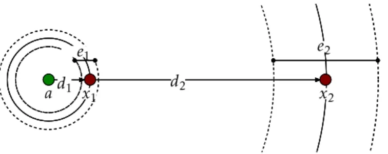
Figure 2.2: Eff_{ects of errors in RSS-based range measurements versus distance.}

Table 2.1: Path Loss Exponent values for diff_{erent environments [}₅₅_]

Environment Path Loss Exponent (PLE)

γ

Free space 2

Urban area cellular radio 2.7 to 3.5 Shadowed urban cellular radio 3 to 5 In building line-of-sight 1.6 to 1.8 Obstructed in building 4 to 6 Obstructed in factories 2 to 3

Using this technique for distance estimation off_{ers the already mentioned benefit of} not needing additional hardware. Consequently, this method saves power compared to others, since additional hardware means higher power consumption.

Localization using RSS based schemes has some disadvantages that cannot be over-looked. First, the accuracy of this methods is severely aff_{ected by shadowing and} multi-path eff_{ects, requiring multiple measurements to deal with them. Second, when there} is an obstacle between two nodes, meaning thatLoScommunication is impossible, the signal suff_{ers greater attenuation compared to its LoS counterpart. This means that in} this situation the distance estimated using the RSS is not a good estimate of the actual distance. Moreover, unlike the first problem, this one cannot be corrected by realizing multiple measurements since the obstacle’s eff_{ects will a}ff_{ect all of them [}₂_{]. Third, the} pa-rametersγ andX in model2.1depend on the surroundings, and obtaining estimates for them might prove to be diffi_{cult and sometimes even impossible. Finally, all sensor nodes} should have their transceivers calibrated so that all of them share the same transmission power, or else, the RSSI values do not correspond to the actual RSS [71].

2.3.2 Time of Arrival

Time of arrival is a ranging method that exploits the proportional relationship between the amount of time a signal takes to propagate from one point to another and the distance between those two points (in this case, sensor nodes). It is possible to estimate distance, provided that the signal’s propagation speed is known, using the following relation:

d=v×t

(35)

2 . 3 . R A N G E E S T I M AT I O N M E T H O D S

ni nj

tj ti

(a) One-way ToA

ni n_j

tj1

ti1

ti2 t_j2

(b) Two-way ToA

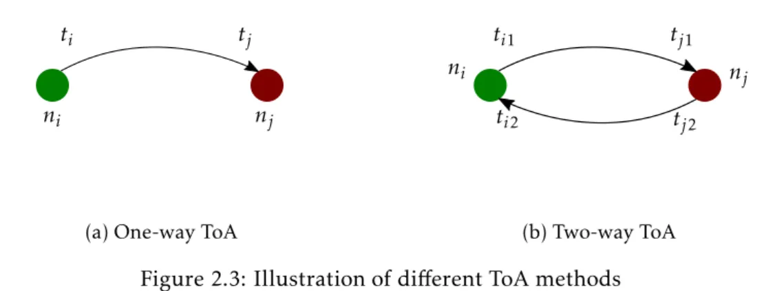
Figure 2.3: Illustration of diff_{erent ToA methods}

whered is the distance,vis the propagation speed, andtis the time taken by the signal to travel distanced. ToA measurements can be done in two distinct ways (see Figure2.3):

One-way or Passive ToA

Passive ToA measures the trip time of a signal from the transmitter nodeito the receiver nodej. The distance is given by:

dij=v×(tj−ti).

For this technique to work, the transmitter must embed the time stamp of transmission in the signal adding complexity and overhead to the signal. Plus, this method relies on synchronization and very accurate hardware to work. This method is the one used in GPS systems [29].

Two-way or Active ToA

In two-way ToA, the receiver node responds to the transmitter node and the round-trip time is used by the latter to estimate the distance between them. The result is sent back to the receiver.

The chronology of the process is the following: Sensor nodei transmits a signal at its local timeti1. The signal reaches sensorj at its local timetj1. After some processing

delay, sensor nodej sends the signal back at its local timetj2. The signal is received back

at nodeiat its local timeti2. The relations are:

Total round-trip time =ti2−ti1

Processing delay suff_{ered at node}_j ₌_t_j₂₋_t_j₁

Round-trip time excluding delay = (ti2−ti1)−(tj2−tj1)

time of flight =(ti2−ti1)−(tj2−tj1) 2

(36)

ni n_j

tj1

ti1

ti2 t_j2

Figure 2.4: Illustration of TDoA.

dij=

(ti2−ti1)−(tj2−tj1)

2 ×v

The disadvantage of this method is that it produces communication overhead, in addition to consuming energy in the process.

Using ToA to estimate distance between sensor nodes is not practical for traditional WSNs. The reason being, if RF signals are used to estimate distance, any small error in time measurement results in a large distance error. In order to obtain accuracy, high precision hardware is needed, which goes against the low-cost, low-complexity premise of WSNs to begin with. If on the other hand, slower propagation signals (e.g., ultra sound) are used to estimate distance, less precise clocks are required. However, sensor nodes have to be equipped with additional hardware which is not desirable either. Nonetheless, algorithms using ToA have been developed [47].

2.3.3 Time Diff_{erence of Arrival}

TDoA is a term often used to describe two diff_{erent things in the context of localization.} In this section however, range estimation methods, which are ways of measuring distance (or orientation), are being discussed. For this reason, we refer to TDoA as a method of estimation distance through the use of two diff_{erent kinds of signal that have di}ff_erent propagation speeds. TheotherTDoA is discussed in Section2.4.1as a geometrical method of computing location.

TDoA uses two diff_{erent kinds of signal to estimate distance. The transmitting node}_i transmits two diff_{erent signals simultaneously or separated by some fixed time interval,} (ti2−ti1). The goal is to use the fact that signals have different propagation speeds, this is

illustrated in Figure2.4. A regular line represents a RF signal, while in order to represent a signal with slower propagation speed a dashed line is used instead. For example, node i transmits a RF signal which is received by nodej at timetj1. Afterwards, nodeiwaits

for a period of timet_i2−ti1, which is also known by nodej, and transmits an ultrasound

signal. Nodej receives the signal at timetj2. With this, the distance can be calculates as:

dij= (vrf −vus)(tj2−(ti2−ti1)−tj1)

(37)

2 . 4 . R A N G E COM B I N I N G T E C H N I Q U E S

wherevrf andvusare the propagation speeds of the RF and ultrasound signal respectively. The most popular user of this technique is the Cricket system [52].

TDoA off_{ers high accuracy if line-of-sight conditions are guaranteed. However,} non-line-of-sight (NLoS)conditions have highly destructive eff_{ects to this measurement method.} Additionally, ultrasonic waves especially are aff_{ected by atmospheric e}ff_{ects such as} tem-perature, pressure and humidity. Finally, this ranging method also requires additional hardware [2].

2.3.4 Angle of Arrival

AoA methods are used to determine the orientation of propagation of a received signal. This methods typically use directional antennas or a special configuration of antenna arrays to estimate the AoA of a received signal [19,45].

When directional antennas are used, they rotate about its axis in order to transmit in or receive from wanted directions. When an array of antennas is used, the antennas’ position in the array is known and used to estimate orientation. The diff_{erence of ToA} of the received signal at diff_{erent antennas is then used to estimate the direction from} which the signal arrived.

The accuracy of AoA techniques depends on the measurement accuracy, that is, on the precision and complexity of the equipment. For example, to achieve high accuracy with antenna arrays very sophisticated ones are required, increasing the cost of sensor nodes and consequently the overall cost of the network. Plus, the required spacing between antennas, so that spatial diversity is guaranteed, often lowers this method’s applicabil-ity. One premise of WSNs is the tiny size of sensor nodes, thus, increasing the size of those nodes for localization purposes might not be an option. Furthermore, multi-path, scattering and NLoS conditions introduces more error to AoA techniques than it does to RSS or TDoA ones [2]. The authors in [44] proposed a APS algorithm that uses AoA measurements. In [42] a technique by which sensor nodes determine their positions in a WSN by obtaining angular bearings relative to a set of fixed beacon nodes is presented. Figure2.5 illustrates how the measurement errors aff_{ect AoA estimation. It is possible} to observe that an estimated angle may be considered a good measurement if the sensors are close to each other. But, for the case when the distance between sensors is high, the same estimated angle may induce to a position which is considerably far away from the real one.

2.4 Range Combining Techniques

(38)

a x1

x2

e1

e2

x y

φ φˆ

Figure 2.5: Eff_{ects of errors in AoA measurements versus distance.}

the existence of noise, whose behavior can be known or not, and the possibility of existing overdetermined systems of equations (more measurements available than the minimum required). [59].

2.4.1 Geometric Approaches

Range and orientation measurements have geometrical interpretations which can be used to compute a node’s position relative to other nodes. Using simple geometric methods such as intersecting enough circles, lines or hyperbolae (in 2-D), results in a position in space [74,78].

Trilateration

Trilateration can be performed using RSS, ToA or TDoA measurements, and it is the most basic and intuitive method [2, 4, 46, 74]. To estimate the position of one node in a 2-D space, that node needs to know the position of three reference nodes and its distance to them (four, in 3-D). Each distance defines the radius of a circle with the respective neighbor at its center. If three of such circles (four, in 3-D) belonging to non-collinear(coplanar) neighbors intersect, the exact location of the node is defined. Figure2.6illustrated how trilateration is performed in a 2-D space.

Triangulation

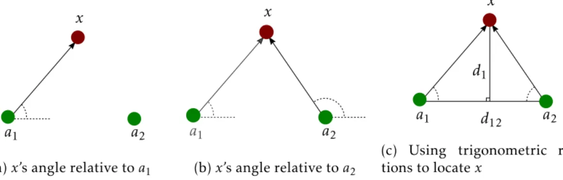
Triangulation uses AoA measurements between the target node and two anchor nodes (three, in 3-D). Each AoA measurement represents a line in a 2-D space (plane, in 3-D), and the intersection of two lines (three planes) give a position in space [2,4,46,74].

Another way of interpreting (in 2-D) can be seen in Figure2.7. Two anchors and a target define a triangle. Using trigonometric relations, the location of the target can be computed using the anchors’ locations and the respective pair-wise AoA measurements.

(39)

d2

d3

d1

Figure 2.6: Illustration of trilateration.

The advantage of triangulation over trilateration is the fact that it requires less an-chors to perform positioning. However, the disadvantages carried by the use of AoA measurement are still present (see Section2.3.4).

a1 a2

x

(a)x’s angle relative toa1

a1 a2

x

(b)x’s angle relative toa2

d12

a1 a2

x

d1

(c) Using trigonometric rela-tions to locatex

Figure 2.7: Illustration of the steps required to perform triangulation.

Hyperbolic Positioning

Often called multi node TDoA1, hyperbolic positioning actually uses ToA as a mean of obtaining distance measurements. In a 2-D case, three synchronized anchors transmit sig-nals at exactly the same time. The receiver (a target) measures the ToA of each incoming signal. Afterwards, the target computes the diff_{erence in ToA from each pair of received} signals,i.e., the pair-wise time diff_{erence of arrival. Each pair of time di}ff_{erences form a}

1_{In reality, ’multilateration’ is the most common term for this technique. However, ’multilateration’ is}

also often used to refer to trilateration generalized for when more than three measurements are available,

(40)

hyperbola in space, and the intersection of two hyperbolae (three in 3-D) is then used to locate the target node [2,4,46,74], this procedure is exemplified in Figure2.8.

d1

a2 _a

1

a3

x

(a) Distance toa1

d1

d2

a2

a1

a3

x

(b) ToA diff_{erence from} _a₁ _and a2

d1

d2

a2

a1

a3

x d3

(c) Hyperbole intersection

Figure 2.8: Illustration of the steps required to perform hyperbolic positioning.

2.4.2 Optimization Based Approaches

Despite the intuitiveness of the geometric approaches, in reality range and orientation measurements are corrupted with errors and noise. Furthermore, there are situations where the number of obtained measurements is higher than the minimum required to perform positioning,i.e., an over-determined system (see Figure2.9). For example, when using trilateration, if a target has five measurements in a non-coplanar case, the inter-section of the resulting five spheres does not result in a single point in space but in an infinite set of possible solutions. In situations like this, a way of determining the solution is minimizing the diff_{erence between the measurements and the known relationships} between the data and the sensor nodes positions [63,76].

Least Squares

Least squares (LS) is a unconstrained optimization problem with an objective function which is the sum of squares. It can be used to solve the localization problem considering that the observation error does not have a known distribution [33,76].

If we consider a set ofM targets in a three dimensional space, their positions can be defined by the matrixX (X_∈R3×M_{). The objective is to estimate}_X_{using observations,}_θ_,

and the known positions ofN anchors,A(A∈R3×N_{). It is assumed that the observations}

are range measurements between all sensor nodes which are within communication range of each other. We can consider that the measurements are function of the target’s and anchor’s positions corrupted by some observation error:

θ=f(X,A) +n, (2.2)

wherenis the observation error andf(X,A) is a known relationship between the node positions and the measurements in the lack of any error. Using this information, we can find the solution which minimizes the squared error between measurements and the

(41)

known relationship,i.e.:

ˆ

X= arg min

X

(θ₋f(X,A))2. (2.3)

Maximum Likelihood

LS assumes that the distribution of the measurement noise is not known. If on the other hand we have such information, it can be used for our benefit. That is, we can maximize the probability density function (PDF) of θ given X, called the likelihood function, obtaining the maximum likelihood estimate (MLE)[33, 76]. Or equivalently, minimize the negative2log-likelihood function3:

ˆ

X= arg min

X {−

log(p(θ_|X,A))_}. (2.4)

Using optimization based approaches to find the solution to the localization problem present a drawback. The problem resides in the fact thatf(X,A) is generally non-linear and non-convex. Considering this, a used solver, more often than not, might not be able to find the solution, i.e., the targets’ positions. The approach to this issue is to apply relaxations or use iterative techniques in order to find an approximation of the true solution.

Recursive methods, such as Newton’s method combined with gradient descent method, are often used to obtain the ML solution [33]. However, since the objective function may have numerous local optima, it is possible that local search methods may get trapped in them. This issue can be overcome by using approaches such as grid search methods and linear or convex relaxation techniques, which can also be used to provide good initial points for more accurate iterative algorithms [35, 36, 48]. Grid search methods solve the ML problem by forming a grid and passing each point of the grid through the ML objective function until the optimal point is found. This approach is suboptimal since it doesn’t search for the solution in a effi_{cient way; the result is a time-consuming method} with computational complexity and memory requirements proportional to the grid size and number of unknown parameters. Less complex are the linear estimators such as the linear least squares. Methods of this type are very effi_{cient regarding the processing time} and computational complexity. Nonetheless they are based on heavy approximations so low accuracy is to be expected, especially in the presence of high noise levels [69]. An-other way of tackling the issue is to employ convex relaxation techniques. The original non-linear and non-convex ML problem is transformed into a convex one. The advantage is that convergence to the globally optimal solution is guaranteed. Still, the obtained convex problem is a relaxed version of the original problem, therefore, its solution may not correspond to the original ML problem’s solution [11].

2_{Negating the function comes from consistency, as conventionally in optimization theory (cost) functions}

are minimized.

3_{The logarithm is a monotonic function, so optimizing a function is the same as optimizing the logarithm}

(42)

d2

d4

d1

d3

(a) Combining noisy distance measurements

φ1

φ2

φ3 φ4

(b) Combining noisy angle measurements

Figure 2.9: Use of an optimization method to combine noisy measurements in overdeter-mined systems.

2.4.3 Hybrid Localization

The most basic approaches of combining measurements rely on just one type of mea-surement. However, recently, hybrid systems that fuse diff_{erent types of measurement} have started to be implemented. The advantage of fusing diff_{erent types of range} mea-surements comes from the increase of available information for algorithms to work with. Hybrid systems take advantage of the strongest points of each ranging method, minimiz-ing their individual drawbacks in the process [18,39].

In [18], Dohertyet al.proposed a way of estimating unknown node positions using connectivity-induced constraints and SDP, additionaly stating that fusing range and angle measurements would be beneficial. The recent works in [6,25, 26] use hybrid systems that fuse RSS with two-way ToA measurements. A. Bahilloet al.proposed a hybrid RSS and two-way ToA scheme where the ToA ranging estimates are used as constraints for the RSS based technique [6]. To combine the measurements, the authors used a least squares approach. The work in [26] proposes a radio frequency identification system for indoor localization. The system uses RSS measurements to determine the bearing of target tags while two-way ToA is used to measure distance. The reason for this lies in the fact that ToA is less sensitive to multipath eff_{ects, and the system is designed to work indoors.} In [25] the authors start by relying on RSS for rough positioning and afterwards use two-way ToA just on the most important links. This two-way, the problem of high communication load that usually comes with the use of two-way ToA is minimized.

Another combination of measurement types is proposed in [37]. The authors design a method which fuses TDoA and AoA measurements to estimate distance and angles

(43)

d2

d4

d1

d3

φ1

φ2

φ3 φ4

Figure 2.10: Use of optimization methods to combine noisy hybrid (distance and angle) measurements.

among sensors. The method’s next step is to adjust the three-dimensional coordinate system based on local measurements and the fact that at least one of the reference sensors is aligned with the earth’s center of gravity (as opposed to using digital compasses). The proposed algorithm is distributed and suitable for practical use on harsh environments.

(44)

reflected before reaching the sensors. In [57], a nonlinear LS estimator is used for lo-calization in visible light communication systems based on light emitting diodes. The authors use AoA measurements as a initial point for an analytical learning rule based on the Newton-Raphson method. Afterwards the algorithm starts using RSS measurements. In [8], Biswaset al.added AoA measurements, to improve their previous approach which only used distance measurements when deriving a semi definite program based localiza-tion algorithm. Tomic et al.proposed cooperative and non-cooperative algorithms for centralized WSNs in [65], which used RSS and AoA hybrid measurements. In [66], the authors establish new relationships between the measurements and the unknown target location by using a spherical coordinate conversion and the available AoA observations, and derive a simple closed-form solution method.

(45)

C

h

a

p

t

e

r

3

Hy b r i d D i s t r i b u t e d A l g o r i t h m s

3.1 Introduction

Two hybrid algorithms (in addition to a generalization) proposed in [68] are presented and studied, in order to ultimately propose a change which allows the creation and con-sideration of a more realistic scenario. The algorithms are distributed, anchor-based collaborative approaches, using hybrid RSS and AoA measurements. In the original work, the authors broke down a non-convex and computationally complex ML localization esti-mation problem into smaller local problems for each target in the network. Afterwards, using the least squares criterion, a local non-convex estimator was derived. This estimator approximates the local ML one for small noise levels. Next, Tomicet al.transformed the non-convex estimator into a convex SOCP estimator and into asquared-range weighted least squares (SR-WLS) one. The authors also generalized the SOCP estimator for the case where target transmit powers are diff_{erent and unknown. The SOCP estimators} were solved by interior-point algorithms, while the SR-WLS was solved using a bisection procedure. While the results show very high localization accuracy in just a few iterations, some strong assumptions were made such as that the network topology remains constant during the computational period. However, this assumption might not hold in prac-tice, especially in dynamic environments where people and/or cars (or other objects) are passing by, blocking the LoS between nodes, or where weather conditions are constantly changing with time.

(46)

C H A P T E R 3 . H Y B R I D D I S T R I B U T E D A LG O R I T H M S

3.2 Problem Statement

The first step to solve the localization problem is to formally state it. The objective is to estimate the coordinates of M sensors (targets), given a priori the coordinates of N sensors (anchors) and pair-wise measurements between the nodes. The WSN is composed ofM+N sensors nodes, with a communication range ofR, randomly deployed over a cubic region of sideB. This WSN can be represented as an Euclidean connected graphG(V,E) with the following properties:

• _V=_{v1, v2, ..., vM+N}is the set of all sensor nodes, represented by the vertexes in the graph.

• e= (i, j)_∈_Eifv_i is within communication range ofv_j, that is, the distance between viandvj is less or equal toR.

We can now label the set of targets and the set of anchors respectively asT (_|T|=M) and

A(_|_A_|=N), where_{| • |}represents the cardinality (the number of elements in a set) of a set. Their locations are denoted byx1,x2, ...,xM anda1,a2, ...,aN (xi,aj ∈R3,∀i∈T,∀j ∈

A), respectively. The sets of all edges that represent target/anchor and target/target connections are defined as _E_A = _{(i, j) : _kx_i−a_jk ≤ r,∀i ∈ T,∀j ∈ A} and _E_T = _{(i, k) : kx_i₋x_{kk ≤}r,∀i, k ∈T, i ,k}, respectively. Lastly, we define a matrixX = [x1,x2, ...,xM] (X_∈R3×M_{) as the matrix of unknown locations that must be estimated.}

It is assumed that the range measurements are obtained from RSS information. When two sensors i andj are within communication range of each other, we can model the signal power received byi,Pij (dBm), as:

P_ijA=P0i−10γlog10

kx_i₋a_j_k d0

+nij,∀(i, j)∈EA, (3.1a)

P_ikT =P0i−10γlog10k

x_i₋x_kk d0

+n_ik,∀(i, k)∈ET, (3.1b)

following [55], where P0i (dBm) represents the reference power at a distanced0 (kxi− a_j_{k ≥}d0, kxi−xkk ≥d0) from the transmitting sensor, γ is the PLE between sensorsi

andj, andnij andnik are the log-normal shadowing terms modeled asnij ∼N(0, σnij2 ), nik ∼ N(0, σnik2 ). For the sake of simplicity and without loss of generality, symmetric target/target RSS measurements are assumed1,i.e.,P_ikT =P_kiT,∀(i, k)∈ET, i,k.

It is assumed that methods like the ones discussed in Section2.3.4are used to obtain the AoA measurements (in 3-D, both azimuth and elevation angles). Before the AoA mea-surements from diff_{erent anchors can be used, digital compasses need to be implemented} in each anchor, since the alignment information is needed [73, 75]. However, a digital compass introduces an error in the AoA measurements due to its static accuracy. For the sake of simplicity and without loss of generality, the angle measurement error and the alignment error are modeled as one random variable.

1_{It is readily seen that, if}_PT

ik ,PkiT, then it is enough to replacePikT ←(PikT+PkiT)/2 andPkiT ←(PikT+PkiT)/2 when solving the localization problem.

(47)

3 . 2 . P R O B L E M S TAT E M E N T

x

y z

aj

xi

αij

φij

dij

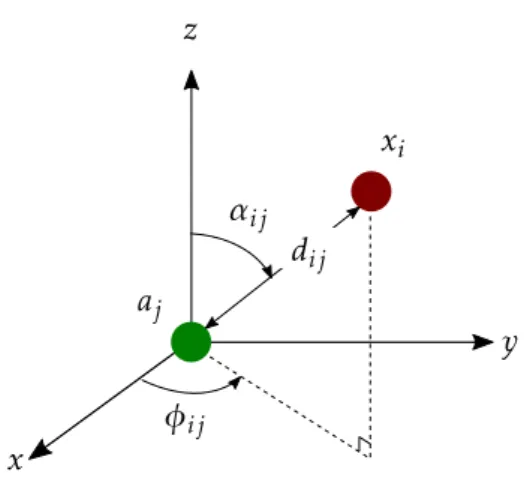
Figure 3.1: Illustration of a target’s relative distance and angles to an anchor.

Figure3.1gives an representation of a target and an anchor locations in a 3-D space. We can definex_i = [xix, xiy, xiz]T as the unknown coordinates of thei-th target, andaj= [ajx, ajy, ajz]T as the known coordinates of thej-th anchor. Additionally,dijA,φAij andαijA represent the distance, azimuth angle and elevation angle between thei-th target and the j-th anchor, respectively. As stated in [49] it is possible to obtain the ML estimate of the distance between two sensors from the RSS measurement model (3.1) in the following way:

b d_ij=

          

d010

P0i−P_ijA

10γ _, _if_j_∈_A_, d010

P_0i−P_ijT

10γ _, _if_j_∈_T_.

(3.2)

We can model the azimuth and elevation angle measurements2by applying simple geom-etry, respectively as [75]:

φA_ij = arctan xiy−ajy xix−ajx

!

+mij, for (i, j)∈EA, (3.3)

and

α_ijA= arccos xiz−ajz kx_i₋a_j_k

!

+vij,for (i, j)∈EA, (3.4)

wheremij andvij are the measurement errors of azimuth and elevation angles, respec-tively, modeled asmij∼N(0, σmij2 ) andvij∼N(0, σvij2 ).

We can now define the observation vectorθ = [PT,φT,αT]T ₍_θ_∈R3|EA|+|ET|_{), where}

2_{The authors in [}₆₈_{] concluded that only the anchors need to perform the respective angle measurements}

(48)

C H A P T E R 3 . H Y B R I D D I S T R I B U T E D A LG O R I T H M S

P= [P_ijA, P_ikT]T,φ= [φA_ij]T,α= [α_ijA]T, the conditional PDF is given as:

p(θ|X) =

3_|EA_Y|+_|ET|

i=1

1 q

2πσ_i2 exp

 

−(θi−fi(X))

2

2σ_i2  

, (3.5)

where

f(X) =                .. . P0i−10γlog10

kxi−ajk d0 ..

.

P0i−10γlog10kxi−_d0xkk

.. . arctan xiy−ajy xix−ajx .. . arccos xiz−ajz kxi−ajk .. .               

,σ=               .. . σ_nij .. . σnik .. . σmij .. . σvij .. .               .

Maximizing the log of the likelihood function (3.5) with respect toXgives us the ML estimate, ˆX, of the unknown locations [33], or equivalently:

ˆ

X = arg min

X

3_|EA_X|+_|ET|

i=1

1

σ_i2[θi−fi(X)]

2_. _(3.6)

The ML estimator in (3.6) has the property of being asymptotically effi_cient,_{i.e., for} large data records it approximates the minimum variance estimator [33]. Solving (3.6), however, is not possible, since (3.6) is non-convex and has no closed-form solution. Never-theless, the LS problem in (3.6) can be solved in a distributed manner by applying certain approximations. The authors [68] proposed a convex relaxation technique leading to a distributed SOCP estimator that can be solved effi_{ciently by interior-point algorithms [}₁₁_], and a suboptimal estimator based on the GTRS framework leading to a distributed SR-WLS estimator, which can be solved exactly by a bisection procedure [7]. It was also showed that the proposed SOCP estimator can be generalized to solve the localization problem in (3.6) where, besides the target locations, their transmit powers are diff_erent and unknown.

3.2.1 Assumptions

The authors in [68] made some assumptions for the WSN (made for the sake of simplicity and without loss of generality), which are enumerated here for the sake of completeness:

(1) The network is connected and it does not change during the computation period3;

3_{We address the scenario where this is not the case in Section}_3.4

(49)

3 . 3 . D I S T R I B U T E D LO CA L I Z AT I O N

(2) Measurement errors for RSS and AoA models are independent, andσnij =σn,σmij = σmandσvij =σv,∀(i, j)∈EA∪ET;

(3) The additional hardware for collecting the AoA measurements is installed at an-chors exclusively;

(4) A coloring scheme of the network is available.

In assumption (1), it is assumed that the sensors are static and that there is no sen-sor/link failure during the computation period, and that there exists a path between any two sensorsi, j ∈V. Assumption (2) is made for the sake of simplicity. Assumption (3) indicates that only anchors are suitably equipped to acquire the AoA measurements, due to network costs. Finally, assumption (4) implies that a coloring scheme is available in order to color (number) the sensors and establish a working hierarchy in the network. More precisely, the use of a second-order coloring scheme is assumed, meaning that no sensor has the same color (number) as any of its one-hop neighbors nor its two-hop neigh-bors [20]-[67], with this approach, energy is saved by avoiding message collision, and the execution time of the algorithm is reduced, since sensors with the same color can work in parallel4.

3.3 Distributed Localization

Note that the problem in (3.6) only depends on the locations and pairwise measurements between the adjacent sensors. Thereby, assuming that estimations for the initial location of the targets are available, ˆX(0), the problem in (3.6) can be divided,i.e., the minimization can be performed independently by each target using only the information gathered from its neighbors. Hence, rather than solving (3.6) directly, which can be computationally exhausting (in large-scale WSNs), the problem is broken (3.6) into sub-problems, which can be solved locally (by each target) using an iterative approach. Consequently, target i updates its location estimate in each iteration, t, by solving the following local ML problem:

ˆ

x(_it+1)= arg min

xi

3_|EA_X_i|+_|ET_i|

j=1

1 σ_j2

h

θ_j−f_j(x_i)i2,∀i∈T, (3.7)

whereEAi ={j : (i, j)∈EA}andETi ={k: (i, k)∈ET, i,k} represent the set of all anchor and all target neighbors of the targetirespectively, and the first_|_E_A_i_|+_|_E_T_i_|elements of fj(xi) are given as:

4_{Note that the network coloring problem may be considered as an optimization problem where the goal}