Implementation of an intelligent sensor for measurement and prediction of solar radiation and atmospheric temperature

(1)

Universidade do Algarve

Faculdade de Ciˆ

encias e Tecnologia

Implementation of an intelligent sensor for

measurement and prediction of solar

radiation and atmospheric temperature

Jo˜

ao Mealha Gomes

Masters in Electronics and Telecommunications Engineering

2011

(2)

Universidade do Algarve

Faculdade de Ciˆ

encias e Tecnologia

Implementation of an intelligent sensor for

measurement and prediction of solar

radiation and atmospheric temperature

Jo˜

ao Mealha Gomes

Supervisors

Ant´

onio Eduardo de Barros Ruano

Pedro Miguel Fraz˜

ao Fernandes Ferreira

Masters in Electronics and Telecommunications Engineering

2011

(3)

Acknowledgments

Financial support for this study was provided by the project ”PTDC/ENR/73345/2006 - Intelligent use of energy in public buildings” through the Centro de Sistemas Inteligentes (CSI) of the Universidade do Algarve, Portugal.

I would like to thank my parents for additional (and vital) financial support!

Many thanks also to:

• my supervisors, Prof. Dr. Ant´onio Ruano and Dr. Pedro Ferreira for their patience and support;

• José Neves,Paulo Luz, Américo Carneiro, Sérgio Miguel and João Lopes from Pub-lirádio®, Rodrigo, Bimbo, Ivo, Amin, Coquet, Sérgio, Igor and Aldric for their technical support;

• NEIUAlg;

(4)

Abstract

The aim of this study was to develop an intelligent sensor for aquiring temperature, solar radiation and cloudiness index data, and use these measured values to predict tem-perature and solar radiation in a near future. The prototype produced could ultimately be used in systems related to thermal comfort in buildings and the efficient and intelligent use of energy resources.

So to incorporate these functionalities, a small and portable prototype was devel-oped, which consisted in: a CCTV camera with a fish-eye lense for sky images aquisition; a computer of format mini-itx with a Linux operating system, for data aquisition and processing; a GPS to enable automatic use independent of the system’s geographical po-sition; a pyranometer for regular measurements of solar radiation; a temperature probe, for regular measurements of outdoor temperature; a shadow band to eliminate the sun’s flare effect on sky images; Arduino, an open source electronics prototyping platform that aquires data from the temperature and solar radiation sensors, as well as processing the data provided by the GPS and controlling the shadow band; neural networks of the type NARX (not developed in this present study), which use the aquired data to forecast the cloudiness index, solar radiation and temperature, in the next four hours.

The system was programmed to aquire data, both from the sensors and the camera, every five minutes.

Keywords: intelligent sensing, temperature, solar radiation, cloudiness in-dexes, neural networks

(5)

Resumo

Este estudo prende-se com a necessidade de desenvolver um protótipo que para além de aquisi¸cão de dados de temperatura, radia¸cão solar e ´ındices de nebulosidade, fa¸ca também uma previsão da temperatura e radia¸cão solar num futuro próximo. Protótipo esse que possa ser utilizado em sistemas visem o conforto térmico, bem como uma utiliza¸cão inteligente de energia.

Por forma a incorporar estas funcionalidades, foi desenvolvido um protótipo de di-mensões reduzidas que incorpora uma câmara de CCTV com uma lente fish-eye, utilizada para a captura de imagens do céu; um computador de formato mini-itx com um sis-tema operativo Linux, que trata da aquisi¸cão e processamento de dados; um GPS, para permitir uma utiliza¸cão automática e independente do posicionamento do sistema; um pi-ranómetro, para realizar medi¸cões regulares de radia¸cão solar; um sensor de temperatura, para efectuar medi¸cões regulares da temperatura exterior; uma banda solar, utilizada para eliminar os efeitos do brilho do sol nas imagens capturadas; uma plataforma de prototi-pagem electrónica open source chamada Arduino, que realiza a aquisi¸cão dos dados dos sensores de radia¸cão solar e temperatura, bem como o tratamento dos dados que provêm do GPS e o controlo do movimento da banda solar; redes neuronais NARX (não desen-volvidas neste estudo), que utilizam os dados adquiridos para fazer a previsão do ´ındice de nebulosidade, radia¸cão solar e temperatura num horizonte de 4 horas. O sistema efectua as medi¸cões dos sensores e a captura de imagens de cinco em cinco minutos.

Palavras chave: instrumenta¸c˜ao inteligente, temperatura, radia¸c˜ao solar, ´ındices de nebolusidade, redes neuronais

(6)

List of Figures

3.1 TSI 440A (Yan (2007)) . . . 21

3.2 TSI 440A sky image . . . 22

3.3 TSI components and power scheme (Yan (2007)) . . . 23

3.4 TSI custom made logic module . . . 24

3.5 Axis 200+ configuration menu . . . 25

4.1 Arduino Duemilanove (image taken from http://arduino.cc) . . . 27

4.2 Logic module state diagram . . . 28

4.3 Shutter speed: 1/10,000; AGC off . . . 29

4.4 Shutter speed: 1/10,000; AGC on . . . 29

4.5 Auto-iris; AGC on . . . 29

4.6 Auto-iris; AGC off . . . 29

4.7 Flow chart for implementation A . . . 30

4.8 External mask . . . 31

4.9 General view of the shadow band . . . 32

4.10 Stepper motor . . . 33

4.11 GPS . . . 34

4.12 Stereographic projection of the sun path for Faro(lat. 37o,lon. −7.6o), ob-tained using a trial version of Solar Tool 2011, Autodesk Inc. 2010 . . . 36

4.13 Spherical representation of point where the sun intercepts the shadow band 37 4.14 Cartesian coordinates representation of Figure 4.13 . . . 37

4.15 Representative triangle of the shadow’s band angle . . . 38

4.16 Used masks . . . 39

4.17 Pyranometer . . . 41

4.18 Pyranometer impedance adjustment circuit . . . 42

4.19 Neural network model . . . 43

4.20 Main script . . . 44

4.21 System . . . 46

5.1 Estimated cloudiness indexes . . . 48

(9)

5.3 CloudSpotter original image . . . 49

5.4 TSI with threshold . . . 49

5.5 TSI original image . . . 49

5.6 NAR cloudiness indexes prediction . . . 50

5.7 Measured solar radiation . . . 51

5.8 NAR solar radiation prediction . . . 52

5.9 NARX solar radiation prediction . . . 52

5.10 Measured temperature . . . 54

5.11 NAR temperature prediction . . . 55

5.12 NARX temperature prediction . . . 55

A.1 Logic Module Wiring: C1 0.1µF ; C2 220nF ; R110kΩ; R210kΩ; R3100kΩ. The connection with a computer is made through a USB cable. . . 67

(10)

1. Introduction

1.1. Motivation

In the field of meteorological data acquisition/estimation, more specifically cloudi-ness indexes, solar radiation an atmospheric temperature, there is room for futher devel-opments. First, there are not a lot of different systems which incorporate, as a package, sky pictures and sensor data. No commercial existing solutions that take photographs for cloudiness studies are portable in a way that they do not allow an easy assemble on the spot. Furthermore, and more importantly, no portable commercial solution incorporates the possibility of forecasting the estimated of measured variables.

This study follows a previous work done by Eduardo M. Crispim et al. (2008), while the estimation is an evolution of A.E. Ruano et al. (2005) and Pedro M. Ferreira and A. E. Ruano (2007). The starting point was the TSI440 from Yankee Environmental Systems, Inc., as it only takes photographs of the sky but does not incorporate any type of sensor, thereby lacking in environmental information.

This study arises from the need to have a device that centralizes a set of tasks -estimates the cloudiness index using photographs of the sky, measures the global solar radiation, measures the atmospheric temperature and predicts the evolution of these val-ues within an horizon of four hours. The previous work done by Eduardo M. Crispim et al. (2008) focuses in the prediction of solar radiation for 30 minutes in future, using multi-objective genetic algorithms for the off-line design of radial basis function neural networks.

This study aims to develop the future in ground to sky imaging systems.

1.2. Goals and Contributions

The main goal of this study is to implement a portable system to measure and predict solar radiation, cloudiness indexes and atmospheric temperature in a four hours horizon,

(11)

based on neural networks prediction models. For this, a prototype had to be developed to take photographs of the sky, measure solar radiation and atmospheric temperature, every minute. Using this data, three Radial Basis Function neural networks will predict the evolution of these variables, over the chosen horizon. As it will be seen during this thesis, several steps were performed towards this goal.

In the end, the prototype was built and validated, constituting therefore the contri-bution of this work.

1.3. Thesis Structure

This thesis is divided into eight different chapters. Chapter 1 contains the introduc-tion of this thesis, as well its motivaintroduc-tion and goals. Chapter 2 introduces the reader to the state of art in acquiring and processing cloudiness, solar and thermal data. Chapter 3 presents the system that became the reference to this study, as well as its main features and drawbacks. Chapter 4 introduces and explains in greater detail the construction of the prototype developed during this study, the considered hypothesis in software and hard-ware, as well as the implementation details and the experimental conditions and results of the system. Chapter 5 presents the validation results. These are compared with the ones from the system presented in Chapter 3. In Chapter 6 the results presented in the previous chapters are summarized, and future work possibilities within this study are also presented/discussed. This Thesis includes also a Reference Chapter and Appendix. The former includes all the used references in the development of the thesis; the latter has all the code, annotations, circuits and specifications of the equipment and software that were not included in any other chapter.

(12)

2. Literature Review

Nowadays there is a global need for decreasing our energy consumption, to ensure that what we get from our natural resources is efficiently used, and that we live in balance with the environment. Increasingly so, efforts in R&D are directed towards this goal. A major field consists in developing intelligent systems capable of integrating environmental data for a more efficient use of resources and sustainable functioning of man-made utilities. In this study, the main focus is on global solar radiation, as it influences the majority of living beings in many different ways. Thus an accurate prediction of its evolution in time is important for several different areas of application, such as the field of renewable energy (see Kalogirou S. A (2001) for an extensive review), people’s comfort in buildings, where possible applications are luminescence control and thermal comfort as Eduardo M. Crispim et al. (2008), among others, proved to be relevant. In the study of global solar radiation, relevant data to be acquired consists in cloudiness indexes, solar radiation and temperature. Not only are these parameters intricately linked, as global solar radiation is usually presented as a time series, making non-parametric methods, such as artificial neural networks good tools for this type of study.

Though no neural network model was developed in the present study, the ones de-veloped by Igor Ant´onio Cal´e Martins (2010) were used. Therefore, in this chapter, special attention is given to the possibilities and different types of data processing when using neural networks, particularly when processing and estimating cloudiness indexes, solar radiation and atmospheric temperature.

2.1. Cloudiness Indexes

The existing research in cloudiness indexes differs in their goal, in how data is ob-tained and how it is processed. Some are concerned with the type of clouds being observed, others only with the amount of radiation filtered. As for data acquisition, the most used technologies are: satellites, ground all-sky imaging systems and spectroradiometers.

(13)

One of the most used geostationary meteorological satellites is the Meteosat, that has been operational since the 1970’s. Many researchers still use this technology, such as Arnout Feijt et al. (2000), to detect clouds, measure temperature and test new models, among other applications. This satellite allows a temporal resolution of 30 minutes and a moderate spatial resolution, which provides an easy way to monitor fast atmospheric pro-cesses. Arnout Feijt et al. (2000) introduced a cloud detection algorithm Meteosat Cloud Detection and Characterization KNMI (Metclock) scheme, which analyses the infra red and visual channels measurements over an area from about 25o_{W to 25}o_{E and from 35}o

to 70oN , covering Europe and a small part of northern Africa. This area was divided in 20 segments for analysis, that were then classified into four different categories: sea, coastal, land and mountainous. In this scheme, each pixel was then classified as cloudy or cloud free by two algorithms, one based on the threshold comparison of the apparent brightness temperature (infra red test) and the other based on the comparison of the threshold of reflectivity (VIS test). Over the sea, the scheme presented quite good results, since the spatial variability was relatively low. However over land, because of high temperature gradients that occur due the variability of surfaces, the results can be misleading. The Metclock differs from other cloud detection scheme’s based on infra-red analysis, in how the temperature threshold is obtained from the infra-red data. One of the most used methods, is the frequency analysis of the spatial distribution of temperatures measured from the satellite. These provide very good results for over sea analysis due to low spatial variability, nevertheless over land analysis the spatial variability is quite high depend-ing on the global zone. As referred in the study, the characterization part of Metclock, used to retrieve cloud cover fraction, optical thickness, emissivity, and correct cloud-top temperature from the reflected sunlight as measured from the VIS channel, is still under development.

Another type of satellite is the moderate resolution imaging spectroradiometer (MODIS), as used by Xiaoning Song et al. (2004) to detect clouds and analyse their images. The study aims to improve cloud removing and precision in remote sensing image recognition. MODIS has thirty six bands with a spectral range from 0.4 to 14µm, twenty visible/near-infra red bands and sixteen thermal infra red bands; but only seven of them were used, the ones sensitive to clouds, aerosol, temperature and water vapour. The area

(14)

used for this study had several singularities, such as vegetation, sand and water, and since these have typical spectrums, it was easy to recognize clouds. The cloud pixel informa-tion was obtained through the low temperature on the cloud top using thermal infra red bands, but the thin clouds were not detectable. When temperatures from land surface and top thin clouds were alike, it was necessary to statistically analyse the eigenvalues of each land cover in the image to know the distribution of values. The thresholds used for automatic cloud detection, were related to time, region and sensor which translates data into a spatial texture, that altogether with a neural network provided an automatic detection method. As for the results of the method, the precision was up to 95%, since it is said that it works quite well in those cloudy pixels that are uneasy to distinguish in naked eye.

Alternatively to satellite observation are the all-sky imaging systems, which promote a more accessible way of cloud monitoring. In the study made by G. Pfister et al. (2003), that aims to monitor the impact of the clouds in the radiation field, without relating it to the temperature, two different all-sky imaging systems were used to measure the total opaque and thin cloud fraction, indicating as well whether the sun was or not covered by clouds. The used all-sky imaging systems are:

Allsky1: developed by the National Institute of Water and Atmospheric Research (NIWA);

Allsky2: also known as Total Sky Imager (TSI) 880 built by Yankee Environmental System, Inc.;

The two systems cover the same field of view, and were placed 300 m from each other, allowing the possibility of using the images for stereographic analysis of cloud height. Both systems use a wide-angle lens, a hemispheric mirror and a shadow band to prevent sun’s reflections. The analysis of the pictures was based on red-to-blue ratio (the ratio of red to blue light in a pixel), since white clouds have a higher red-to-blue ratio than blue sky. A red-to-blue threshold was then used to determine whether a pixel is cloud or clear sky. There was also an estimated fraction cloud cover, that was given by the number of cloudy pixels divided by the total number of pixels in the field of view. Besides the comparison of the two systems, which was done through the comparison of ± 67000 images, where in about 80% of the images the absolute difference in the total and opaque was less than 10%, there was an effort to relate the cloud effect over the solar

(15)

irradiation. Despite the fact that the cloud fraction is an important element in the amount of solar radiation that reaches the surface, it was not possible to relate the cloud coverage alone to the solar radiation, even when the sun was obscured. Cloudiness indexes were not sufficient to explain the radiation field. Nevertheless it was shown that this type of technology proved to be a good way of making long term measurements, and also to con-tinue studying the cloud coverage with high temporal resolution. It is also important to mention that this study was an important starting point for the use of this type of systems.

A different type of on ground all-sky imaging, is the one used by A. Cazorla et al. (2007), which aims for aerosol characterization using neural networks. The study is based on the principle that aerosols affect Earth’s radiation and the temperature field by chang-ing the energy balance and solar distribution in the atmosphere. The instruments used in this work were: an all-sky imager developed by Atmospheric Physics Group (GFAT), to provide images of the whole sky dome in daytime for cloud characterization; a Peltier sys-tem to control the sys-temperature of the syssys-tem; a solar shadow syssys-tem, a 2AP Sun Tracker (by Kipp & Zonen), that must cover the camera lens every moment. To obtain a charac-terization of the aerosol optical depth (AOD) they used a sun-photometer CE-318-4 (by CIMEL Electronic). Two radial basis network were used, one for estimating the AOD, and another for the α estimation (characterizes the spectral features of the aerosol, ˚Angstr¨om (1964), and is related to the size of the particles, Shifrin and K.S. (1995)). The results were compared with the CIMEL CE318 sun photometer, and for the AOD the results are in the limits of nominal precision of the CIMEL CE 318; for the α parameter about 80% of the cases have deviations of below 0.1, which is also between the limits of nominal precision. But there is an uncertainty to the precision of the system, and the developed neural networks were quite sensitive to the quality of the data used for the training.

In a more recent work by Francisco J. Olmo et al. (2008), the retrieval of optical depth using a CCD camera was studied, using the same system as A. Cazorla et al. (2007). The study uses a real-time iterative procedure. The first method did a cloud classification of pixels derived by a neural network (using a multilayer perceptron model), reconstructing spectral sky radiance at zenith by a linear pseudo-inverse spectral estimation algorithm, and finally, deriving the optical depth at 550nm using radiative transfer code. In this

(16)

method the clouds were classified based on three parameters, mean of the pixel and its neighbours in the red and blue channels, and the variance of the pixel and its neighbours in the red channel. The information obtained was the percentage of thin clouds, oktas1

for opaque and thin clouds, the percentage of opaque and thin clouds in every octant, and the sun position in the octant. The second method was used to obtain real-time sky radiances (spectral power distribution) at zenith, from 380 to 780 nm, by means of the pseudo-inverse spectral estimation algorithm, which provided a spectral radiance for each pixel 1280 × 1024 image in real time and required a training set. The training set was based on grouping the similar spectral radiances, according to their distances mea-sured by the colorimetric and spectral combined metric, defined by M. A. L´opez- ´Alvarez et al. (2005). The third method showed that it is possible to recover zenithal sky radiance spectra, with a reduced number of broadband spectral filters used in the CCD camera. The authors of this study claim that the methodology presented solves the strong for-ward scattering problems associated with the large particle load in neural networks. As the only training set concerns the spectral sky radiance reconstructions, the absolute ra-diance calibration was not necessary, and the training set does not depend on the location.

Based on radiometric data the work of H.F. Assun¸cão et al. (2007), used 5 minutes averaged values of global and indirect solar irradiance and daily values of sunshine du-ration, considering four types of cloud reflection, clear sky, sun reflecting in clouds, sun partially covered and sun totally covered. With the developed algorithm, it was possible to estimate the daily and hourly conditions of the sky. Previous work had been done on this subject, such as J. Calbó et al. (2001), D.H.W. Li and J.C. Lam (2001) and A. Orsini et al. (2001), which catalogue the clouds in different forms and with different time estima-tions. The method used in this study to characterize the sky was based on solar irradiation values that allows the estimation of the cloudiness indexes for the past five minutes. H.F. Assun¸cão et al. (2007) chose this time interval based on H. Suehrcke and P.G. McCormick (1988) work, that observed that the frequency distribution for 5 minutes-averaged solar irradiance values is similar to the frequency distribution of instantaneous values and con-cluded that hourly and daily values of solar irradiance do not represent appropriately

1_{Unit used to define the clearness of the sky. Each okta represents one eight of the sky covered by}

(17)

the statistical properties of instantaneous values. The data acquisition for this study was made in Botucatu in the state of S˜ao Paulo, Brazil; the global solar irradiation was made with a pyranometer of spectral precision (PSP), and direct solar irradiation was measured by a pyrheliometer coupled to a sun tracker model ST-3, manufactured by Eppley Inc. The measurement period was six years, from 1996 to 2001. The proposed algorithm was based on the principle that short term variations of cloudiness were due to changes of the relative optical mass of air. Different frequencies were used for clear and cloudy sky, but it was also necessary to set boundaries to the different types of categories, that according to M. Jurado et al. (1995), can be mathematically justified and are well defined. The algorithm consists in a matrix of four columns and the number of lines corresponds to the number of observed indexes during a day, made to obtain the real duration of the day. The collected datum was compared with a recording device from Campbell-Stocks, with few errors. The authors also suggest that this algorithm is to be used only in places where there are solar irradiation records, with at least five years.

The study made by Calb´o and Sabburg (2008), show a method that analyses and recognize clouds according to their patterns. In order to achieve that purpose, pictures from two different devices were used:

• the TSI (Total Sky Imager), has a field view of 160o_{, and the photos are 352 ×288}

pixels in JPEG format. After capture, the photos were transformed to 256 × 256, through a bilinear interpolation using the MATLab® software.

• the WSI (Whole Sky Imager), is a colour digital camera with a fish-eye lens, provid-ing a field of view of 180o_{, that aims to the zenith. The captured photos are 768×576}

in BMP format, although it is referred that the JPEG format with a compression of 80% was better for the image digital processing.

Besides their own experience in the field, the authors also based this study on pre-vious works of Buch et al. (1995), defining 8 conditions to be used in cloud classification. These are not based on the classical classification of clouds, but on the visual aspect of the cloud instead. The photos were characterized through their texture, analysing the his-togram properties. These process can be applied to gray-scaled pictures, that is pictures whose pixels information is represented by a single value. Since the captured pictures had

(18)

three components, red, green and blue (RGB), they had to be transformed to gray-scale pictures. Two transformed pictures were used, one had the red component transformed to blue and the other only had the value of the intensity, given by (R + G + B) ÷ 3. Cloud pattern was analysed in frequency using a Fourier transform, based on Gonz´alez et al. (2004) work. It is important to mention that the initial values are real, and that the spectral power is symmetric relatively to the origin. Since the power spectral functions from different types of sky are different between them, it was necessary to identify simple characteristics in spectral power, to identify each type of cloud. These characteristics are:

Correlation with clear (CC) sky: quantifies and compares the spectral power of the analysed image, with a reference (spectral power of image with clear sky). The CC value is the linear correlation coefficient between the logarithms of the two power spectral functions, between 0 and 1. The bigger this value is, the more homogeneous is the sky.

Spectral intensity (SI): depending on the presented cloud patterns, there will be more or less spectral power.

Since the previous methods only analysed the image pixels, and since there was not a distinction between cloud pixels and clear pixels, other characteristics were added allow-ing a better recognition of each type of sky. This distinction was made usallow-ing a threshold in the image R/B, and its value was calculated using a MATLab® script, value which was based on the the picture histogram. According to this study, it is possible to recognize sky patterns subsequent cloud classification. It is mentioned, that during the research of the study, there were explored two different characteristics: Fourier transform, one of most promising approaches to cloud-pattern recognition, became limited when tried to summa-rize a limited number of values, the information contained in the FFT; pixel distinction, could have led to better results if the value of threshold was changing according to the position of the pixel.

In the study made by Atsu S. S. Dorvlo et al. (2002), a set of neural networks is presented that estimated the cloudiness indexes using latitude, longitude, altitude, light intensity and month of the year. They used radial basis function neural network (RBFNN ), the learning method involved the input/output data to exploit the next

(19)

pa-rameters: the network inputs, the bandwidth of the Gaussian function, and the weights between networks neurons and output layer. One of the techniques used to get the de-scribed parameters was based on fixed RBFNN. This RBFNN has random selection for the centres in the set and the width of Gaussian radial basis function was expressed in terms of the maximum distance between the chosen centre and the number of centres. To train this neural network the author used a back propagation algorithm implemented in the neural networks toolbox of MATLab®.

Another neural network used was the multi layer perceptron (MLP ) network, which consisted in one input layer, and one or more hidden layers. The architecture used in this model had five neurons in the first layer, one hidden layer with sigmoid activation function, and a output layer with a linear activation function. This network training was made using a back propagation algorithm belonging to the neural network toolbox (trainbr ). In the end, the final network was implemented with one, two and three hidden layers, and the best results were selected using the mean square error.

The data sets were collected from eight meteorological stations during ten years, and were used to train three MLP and one RBFNN neural networks. The output parameter was the cloudiness index. To get the solar radiation, the author used this index and multiplied it by the maximum radiation index.

It is said in the study that both network types had reasonable results, but the RBFNN model was preferred due to its best results and smaller computational time.

In this thesis, the implemented sky classification method was developed on the study of Pedro M. Ferreira et al. (2010) and the ANN’s used to predict cloudiness was developed on the study of Igor A.C. Martins et al. (2010).

The sky classification method was implemented using a new approach based on ANN’s alternatively to the common threshold method. This implementation was also compared with three different methods: fixed threshold, RCT method, Otsu’s method and a Neural Network method. A common approach in all methods, is the calculation of the threshold value on a given pixel intensity scale. The testing of this approach involved several intensity scales. On the original RGB image the red channel were considered, and were also considered the grayscale images after a transformation being performed.

(20)

This transformation consists on the conversion of the original RGB image into the Hue-Saturation-Value (HSV) colour model, setting the value channel to 1 for all pixels, and converting the transformed image back to RGB. The transformation applied to the value channel, has an equalization effect on the pixels of the luminosity, since the colours on the HSV colour model become more distinct. The converted RGB images have an improved contrast within the red channel, which allows a clearer distinction between the clear sky and the cloud pixels. The fixed threshold method is based on a histogram analyses in order to identify the best single threshold value to be applied to every image of the used set. The RTC method consists on an histogram iteration form, presented by Trussel (1979), of an iterative thresholding algorithm proposed by T. Ridler and S. Calvard (1978). This method evaluates a unique threshold from each image, assuming a bimodal histogram, being the threshold T = (µ0 + µ1)/2. The µ0 and µ1 are the means of each of the two

components of the histogram separated by the threshold. The Otsu’s method, proposed by Otsu (1979) , consists on searching the pixel intensity scale for the threshold that maximises the inter-class variance of each component of the histogram. In the Neural Network method an attempt was made to identify a Radial Basis Function (RBF) Neural Network (NN) image thresholder using a Multi-Objective Genetic Algorithm (MOGA) developed by C. Fonseca and P. Fleming (1998). The NN’s were trained by the Levenberg-Marquardt algorithm using a modiffed training criterion exploiting the nonlinear-linear RBF NN topology (P. M. Ferreira and A. E. Ruano (2000); Ferreira et al. (2002)). In this method the set of 410 images was broken into three sub-sets: the training set (290 images) for NN training; the testing set (60 images) for generalisation testing; the validation set (60 images) to evaluate the NNs after the MOGA execution. From all the images and from the performed transformations, a total of 69 features were extracted. First, from the original RGB image the HSV and Hue-Saturation-Lightness (HSL) images were obtained. Secondly, on the HSV and HSL images the V and L channels were set to 1 and 0.5, respectively, and these transformed images were converted back to RGB mode generating two additional RGB images. Finally, from each RGB mode image a gray intensity image was generated. This resulted in a total of 7 different images and 17 distinct intensity channels. From each of these, the sample mean, standard deviation, and skewness were extracted. Additionally, from the red and gray intensity channels (6 in total) histogram, the most frequent, first non-zero, and last non-zero intensity levels were also extracted.

(21)

The NN structure (set of input features and the number of neurons) was selected using the MOGA in a similar way to that presented in P. M. Ferreira et al. (2003). Two objectives were setup for minimisation: the training and generalisation NN output (Root Mean Square) RMS errors. The NN revealed an improvement in accuracy of approximately 50% when compared to the best results obtained by the remaining methods.

The cloudiness prediction methodology used the RBF NN image thresholder se-lected in the identification experiment described in the previous study, cloudiness time-series were estimated by feeding the NN with the features extracted from consecutively acquired (1 minute sampling interval) images, and applying equations 1 to 4 for each image and corresponding estimated threshold. Which was done for a three months peri-ods: October, 2004; February, 2005; and May, 2007. The correlation of measured global solar radiation to the cloudiness was also inspected. These time-series were afterwards employed in the identification of RBF NN cloudiness predictive models. As these were meant to be employed in a global solar radiation prediction scheme which operates on the basis of a 5 minute sampling interval, the cloudiness time-series were averaged over 5 minute consecutive periods, thus generating smoothed time-series synchronised with the solar radiation data. The experiments for the identification of RBF NN cloudiness predictive models by means of a MOGA, followed the same principles outlined in the previous section for the NN image thresholder. In this case the NN cloudiness predictive models were identified as autoregressive One-Step-Ahead (OSA) predictive models which, for a given instant k, were iterated in a multi-step fashion to generate predictions from instants k + 1 to k + ph, where ph is the prediction horizon, in this case set to 48 steps corresponding to 4 hours. The MOGA was employed to evolve a preferable set of models whose number of neurons and selected input terms optimise a number of pre-specified goals and objectives. In this case the MOGA chromosome, the cloudiness auto-regressive predictive model, are a collection of delayed output signals, together with the number of neurons. The input terms considered were selected from the delays within the period of the past 24 hours.

To assess the models performance three objectives were used: the RMS, the OSA error and the third objective was computed on the basis of the long-term model prediction error taken from the multi-step model simulation over the prediction horizon. The best

(22)

model structure has 6 neurons and employed 13 input terms, and also corresponds to the best one in the preferable set in terms of the long term prediction objective, the minimization of the summed RMS prediction error.

Thus for cloud detection, satellites tend to be more used, as shown by Arnout Feijt et al. (2000),Xiaoning Song et al. (2004), Patrick Minnis et al. (2008) and B. H. Kahn et al. (2008). Nevertheless, ground to sky imagers tend to be a cheap alternative allowing images with greater resolutions, the frequency between each new image being higher than the satellites and also providing more focused results, as shown by Buch et al. (1995), G. Pfister et al. (2003), A. Cazorla et al. (2007), H.F. Assun¸c˜ao et al. (2007), Calb´o and Sabburg (2008) and Francisco J. Olmo et al. (2008).

2.2. Solar Radiation

Solar radiation estimation is not a trivial subject, specially if zones with a complex topology are considered, such as mountain cases, where it is difficult to support economi-cally and maintain the equipment. Another problem in this type of terrains is the number of variables involved; these require a denser neural network. There are a few studies in this area, such as J.L. Bosch et al. (2008), who performed a study in which the performance of active and passive energy systems are analysed and J.C. Winslow et al. (2001), who devel-oped a model of daily solar irradiance estimated from air temperature and precipitation data. In this last approach, the best results were obtained through extrapolation/interpo-lation of the acquired data in a station near of the study location, but even there it was difficult to take problems such as terrain complexity, into account.

Other studies also explore the benefit of using neural network instead of an empirical model, such as the study performed by Jérôme G. Fortin et al. (2008), which considers also two classical approaches to simulate the propagation of solar radiation on earth surface developed by Tymvios F.S. et al. (2005). Besides the classical methods, the solar radiation could be estimated by radiation measurements interpolation, as studied by Y. Xia et al. (2000), or by satellite images analysis, as studied by Lèfevre M. et al. (2007).

(23)

the HS model developed by Hargreaves G.H. and Samani Z.A. (1982), which is a simple empirical model to simulate daily solar radiation received in an horizontal surface to estimate the evapo-transpiration; and the MH model developed by Mahmood R. and Hubbard K.G. (2002) that uses a different approach in the empirical model, in which the transmissivity is a function of the day of the year, and the daily solar radiation received by the surface is correlated with temperature amplitude and extraterrestrial radiation. The latter is identical to the previous, the main difference being the unbiased characteristic. These models were optimized using a non-linear standard unrestricted scheme.

The neural network method used was the MLP, trained with the optimized Levenberg-Marquardt Back-Propagation Optimization with a Bayesian regulation. The selected in-puts were the extraterrestrial radiation, the day of the year and maximum and minimum air temperature. The best performance was achieved with eight neurons in the hidden layer. The collected data was provided by eleven meteorological stations, and consists of temperature and solar radiation, where the data from six of them were used for trainning and optimizing the empirical method. The other 5 stations were only used for testing. Each station gave about 225 data sets of solar radiation, in the years 2004 and 2005. Each variable had 2522 observations, 1385 of them to train the network and 1137 to validate it. The empirical model that obtained the best results was the HS, and even after the error optimization, the errors obtained by this model were greater than the results ob-tained by the second best neural network. These results were almost unbiased. The MLP formulation had enough flexibility to explore a wide range of multivariate regressions in a single step. This advantage prevails over empirical models like HS or MH where the formulation structure was fixed beforehand. Furthermore, the non-linear property of the MLP activation function was particularly valuable for reproducing the behaviour of a natural phenomenon like surface incoming solar radiation and its relation with common meteorological variables.

The model used in the study of J.L. Bosch et al. (2008) used artificial neural net-works, since these methods allow more accurate results in the solar radiation forecast and estimation than other models. The data used was collected by 12 stations localized near the Sierra Nevada, in the city of Hu´eneja in Granada, Spain. These stations collected solar

(24)

radiation using LICOR 200-SZ pyranometers between 2003 and 2005, with an interval of 2.5 minutes. In the study, the data of one of the 12 stations were chosen be the reference of the artificial neural networks, and the data of the remaining stations were used to generate comparison values. The artificial neural network used was a MLP with one hid-den layer, due to its simplicity; the activation function was the hyperbolic tangent. In this study a method is presented, Automatically Relevant Determination (ARD), based on the Bayesian structure (see G. L´opez et al. (2005)) for determining the structure of artificial neural networks. This method limits the complexity of the networks by identifying the variables’ relevance, and avoids the data separation in subsets, therefore allowing the use of the whole data for training. The results were demonstrative and proved that the day of the year and cloudiness index are very important to solar radiation forecast and esti-mation in these conditions, since these variables proved to be vital for the results accuracy.

The study made by Eduardo M. Crispim et al. (2008), also aims for the solar ra-diation forecast, based on sky image acquisition and solar rara-diation measurements. The artificial neural network types used were RBF composed by three layers. The input layer was composed by the sensor inputs, i.e., by the data from the sensors. The second was an hidden layer composed by several neurons chosen by a MOGA, and the third and last layer had a neuron that corresponded to the output. The artificial neural networks’ learning was performed in two parts: the first, in which an unsupervised procedure, OAKM (optimal adaptive k-means clustering) was used to compute the initial position of the centres, its spreads being computed by a simple algorithm. The second part consisted in the training method, through the LM algorithm. To verify the influence of the cloudiness index on the solar radiation forecast, three methods were compared, one without cloudiness index and two others with a different cloudiness index as exogenous input. One of the NARX models had in account all sky and the other just an ellipse area near the sun. The device used to acquire sky images is a Total Sky Imager (TSI), through a CCD camera. This device has a black strip to protect the CCD from the reflected sun on a concave mirror. After collect-ing the images, these are processed to get the cloudiness index (in percentage). The sky was classified as clean sky, clouds with low density level and high density level. The TSI system has an algorithm that classifies the sky, but results were unsatisfactory, especially when the sky had a different hue; for example, when the sky is completely covered with

(25)

clouds, the algorithm presents a result of 0% of clouds, i.e., clean sky. To determine the cloudiness index, two NARX models with different type of cloudiness index were used. These models were later compared with a NAR model. To build a realistic model of solar radiation three different models were used: a NARSR model; a NARX model, with the PCS values as exogenous input; and a NAR model. The data used to train the networks had 10080 points extracted from six days, and the validation set used data from four days, with a total of 7200 points. The solar radiation values were measured with a pyranometer. The lag terms were chosen by the MOGA, employing also an heuristic relation which took into account the solar radiation variation through time, and the relation between the solar radiation and the cloudiness indexes history. The model evaluation was achieved using the Root-Mean-Square of the one-step-ahead training errors (OSATE), of the generalized set (OSAGE) and the RMSE long time forecast. According to the results in the study of Eduardo M. Crispim et al. (2008), the cloudiness index is a relevant parameter in the solar radiation forecast; however the capture methods are not optimized and result in large errors in the cloudiness index determination.

In this thesis, the solar radiation forecast follows precisely the used methodology in the study of Igor Ant´onio Cal´e Martins (2010). Similarly to the previous mentioned studies, MOGA was employed in order to identify the ANN’s input-output structure. The solar radiation data was acquired using a 1 minute sample rate and then re-sampled ap-plying a 5 minute average over the entire data set. The available inputs in MOGA, the lagged solar radiation values, were taken from the past 24 hours. The considered inputs were, all the lagged terms from the most recent 8 hours, inputs taken at 10 minute in-tervals in the following 8 hours and the input terms taken at 15 minute inin-tervals for the last 8 hours. Such choice was made, since the radiation value near the forecasted instant is more important than the values taken in the previous 24 hours. As for the NARX model, the exogenous input terms considered were extracted from the previous 4 hours to the prediction instant. The number of neurons of the models was restricted to range from 2 to 16 and the number of input terms was restricted to lay in a range between 7 and 32. The ANN training method used was the LM algorithm using a modified criterion exploiting the non-linear/linear topology of the RBFNN, and the stopping criteria used was early stopping. The NARX model and the exogenous inputs considered used a re-cursive multi-step prediction, an approach usually called the Minimum Error Prediction

(26)

(MEP). As for the results, the long term forecast was considered to compare the NAR and NARX approaches. The best result for the NAR system was achieved with a NN with 22 input terms and 6 neurons in the hidden layer. This structure achieved an RMS error of about 80W/m2 _{at the four hour ahead prediction. For the NARX system, the best RMS}

error at the four hour horizon was around 50W/m2_{. This represents an error decrease of}

approximately 30%, relatively to the NAR model.

2.3. Temperature

The study of Kostas I. Chronopoulos et al. (2008) has the purpose of obtaining ANN’s models to estimate meteorological data values in areas with sparse meteorological stations. This study relies on the need of having available meteorological data in the required spatial resolution, which might no be available due to the complex terrain of the studied area, or due to the sparse network of meteorological stations in the major area of the study. The goal of this study was to develop and apply ANN’s models to estimate atmospheric temperature as a function of the corresponding values of one or more reference stations. The application site is the canyon of Samaria, located on the south-west Crete Island, Greece, covering a total distance of 18 km. The data set used consists of measured mean hourly temperature data from 4 meteorological stations, which were HOBO® type of Onset Computer Corporation. The sensors were protected with radiation shields and were placed on trees about 1.5m above ground. All measurements were taken every 10 minutes and then were averaged to hourly values. A statistical model (multiple regression model), was used as comparison to test the performance and evaluate feasibility of the developed ANN’s. The data set used consists on a total of 1550 hourly observations. The data was divided into two separate overall data sets, the first data set was used for training, while the second was used for testing and consisted on 550 hourly observations. The variables are the mean hourly temperature data from the four stations and the mean hourly relative humidity data from two of the stations. An ANN model was developed, a multilayer preceptron (MLP) and a statistical model, multiple linear regression (MLR). The MLP was trained with a back propagation algorithm, and the network consists on 1 hidden layer and 3 nodes. The method uses the final weight as initial weights of the validation networks to take into account the problem that a network

(27)

trained with all of the known data set may not be identical to networks trained with subsets of the data. On the MLR, the regression coefficients represent the independent contributions of each independent variable to the prediction of the dependent variable. The evaluation of the performance of the results obtained using the MLP and MLR, was done through two different criteria: the determination coefficient between the observed and estimated values (R2_{) and the Mean Absolute Error (MAE). The evaluation of the}

preliminary results of an ANN model used in the present study to estimate air temperature in areas where meteorological stations were sparse, showed that fair to very good air temperature estimations may be achieved depending on the number of the meteorological stations used as reference stations. The comparison of the ANN model results with the results obtained from the MLR model, showed the better performance of the ANN model. In addition, it is mentioned that the ability of ANN models to take into account any non-linear relationships among meteorological parameters, may provide advantages over traditional methods.

The control of the environment inside a greenhouse, is also an import topic when studying the prediction of atmospheric temperature, such as the study preformed by Irineo L. L´opez-Cruz et al. (2007), in which a dynamic linear model of auto-regression with exogenous variables was developed to predict the air temperature inside the greenhouse. And also the study performed by P.M. Ferreira et al. (2005), where a radius basis function (RBF) model was developed in order to predict the greenhouse temperature and humidity.

The study developed by Irineo L. L´opez-Cruz et al. (2007), aimed for an evaluation on the methodology used to generate ARX models in order to predict the air temperature of a Mexican greenhouse with natural ventilation. The greenhouse has 1080m2 _{and is}

located at an altitude of 2244m in the experimental field Tlapeaxco of the Universidad Aut´onoma Chapingo in M´exico. The meteorological and input variables were temperature, relative humidity, solar radiation and wind speed. They were measured during 3 months, using two Davis® Weather automatic meteorological stations. The output variable was the air temperature inside the greenhouse. Samples were taken of the input and output variables of the model every 5 minutes during a crop cycle. To determine the structure of the best model, 100 000 ARX models were evaluated using the information criteria and final prediction error of Akaike (1974). The adjustment between the simulated and

(28)

observed temperatures, and the residual analysis, indicated that ARX models of second degree or above, adequately predict the behaviour of the temperature inside the green-house. It is said, that the obtained ARX models had a fit of more than 70% over the group of data of estimation and validation, and also that the models also satisfied the residual analysis.

The study developed by P.M. Ferreira et al. (2005), applied a MOGA to identify the radial basis function neural network coupled models of humidity and temperature in a greenhouse. This study arise from a similar need as the study of Irineo L. L´opez-Cruz et al. (2007), since the greenhouse temperature and humidity are the two most important environmental variables, that affect the crop production. The data used in study was acquired with a sampling rate of 1 minute in a plastic covered greenhouse, and was collected during 12 days. The variables involved were the greenhouse relative humidity and temperature, the outside temperature and solar radiation. The wind speed and direction was not considered, since the authors did not have any information on the greenhouse’s opening state, and it is mentioned that in previous studies the MOGA discarded these variables from the model. The number of points used was reduced by applying a 5 minute average over the entire data set, and afterwards, due to the different scales in the variables considered all were scaled to the an interval between 0 and 1. The resulting data was split into three different data sets, model training, generalisation testing and validation. The RBF NN’s were trained as one-step-ahead (OSA) predictors by an algorithm based on unconstrained deterministic optimisation employing a Levenberg-Marquardt method. Early stopping was used to terminate training. In the MOGA each individual was a pair of humidity-temperature models. Both models structure were a Non-linear auto-regressive model with exogenous inputs (NARX). The quality of each trained NN was assessed by its prediction performance over an horizon of 3 hours (36 steps) using the generalized testing data set. To reduce the computational time, the authors computed the prediction starting at one hour intervals, which resulted in 96 prediction horizons. The respective error of each prediction was measured using the root mean square error (RMSE). The obtained networks had 6 neurons and 11 inputs for the humidity model, and 2 neurons and 29 inputs for the temperature model. The study presents good fittings for the prediction in 1, 18 and 36 steps ahead. The mean and maximum absolute error values obtained for humidity and temperature were 3.0383%, 24.5791%, 0.8434o_{C, and 6.1402}o_C.

(29)

In this thesis, the temperature forecast follows precisely the used methodology in the study of Igor Ant´onio Cal´e Martins (2010). Similarly to the previous mentioned studies, MOGA was employed in order to identify the ANN’s input-output structure. The sampling rate used in data acquisition was the same as for the solar radiation model mentioned in the previous section, as well as the temperature input terms selection. In this model the exogenous input is the solar radiation, whose lagged terms were extracted from the previous 6 hours to the forecasting instant. The number of neurons for the models was restricted to the range from 2 to 20. The training methodology, the stopping criterion and network type were the same mentioned in the previous section. The MOGA population size was set to 100 individuals, with the introduction of 10 new individuals randomly generated. As for the results, the best long term temperature forecast produced a mean-squared error of approximately 1.5o_{C on the four-hours horizon, having an asymptotic}

behaviour right above this value. The NN model has 19 input terms and 4 neurons in the hidden layer. As a final remark, the author mentions that the obtained result will deteriorate due to error propagation.

(30)

3. Background

3.1. Summary

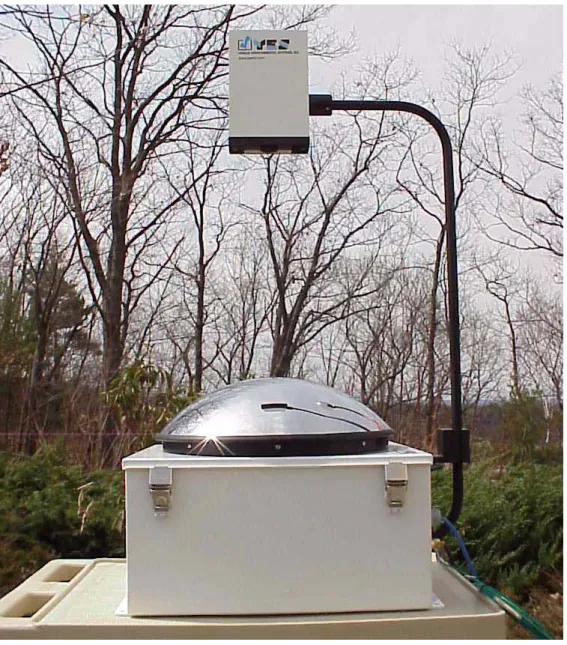
This project took as a reference an industrial total sky imager used in the Centro de Sistemas Inteligentes (CSI) laboratory in UALg, the T SI440A from Yankee Environ-mental Systems, Inc. (see Figure 3.1).

Figure 3.1: TSI 440A (Yan (2007))

For a brief explanation of the system it will be separated in three different parts: its structure, the logic module and the Axis200+ ip camera. Below is a description of the

(31)

main characteristics of the system (see Yan (2007) ): Imager resolution: 328 × 288, 24-bit colour;

Sampling rate: variable, with a maximum of one image every 10 seconds;

Operating temperature: −30o_{C ⇔ 34}o_C;

Weight: approximately 23kg;

Power: 110/220 VAC;

Data storage: disk on local computer or remote computer over a full-time TCP/IP connection

3.2. TSI Structure

The TSI structure has two parts (see Figure 3.3(a)), a chrome-plated steel mirror on which the whole sky is reflected on, and an arm that holds an Axis200+ ip camera that captures the reflection of the sky in the mirror (see Figure 3.2). The acquisition of the images is done by accessing the ip camera’s web server.

(32)

in case of power failure. The Figure 3.3(b) shows the setup used.

(a) General view

(b) Focused view

Figure 3.3: TSI components and power scheme (Yan (2007))

In order to achieve the desired results, the system must not have any visual inter-ference. It must be placed in a high place, and even there, the responsible for its assembly must check if it suffers or not from visual interference. If it does, a software mask must be applied in order to not compromise the results.

3.3. TSI Logic Module

The logic module of the TSI was replaced by a custom made module (see Figure 3.4), due to the failure of the original one. The custom made module did not add any functionality besides the existing ones. The module is responsible for the calculation of the azimuth in degrees for the sun’s position, and depending on its value, the chrome-plated

(33)

steel mirror rotates until it gets to the azimuth position. The azimuth value depends on the geographical coordinates, these must be hard-coded in its calculations.

Dc Motor Arduino Output Ethernet Power Output rs232 Driver Dc Motor Driver

Figure 3.4: TSI custom made logic module

This system uses an encoder from US Digital to retrieve the position, and a dc motor to move the chrome-plated steel mirror. The following equipment was used to rebuild the logic module:

Arduino Duemilanove: core of the logic module;

Arduino Ethernet Shield: retrieve date and time from an NTP server;

MAX3232CPE: interface serial communications between Arduino and the US Digital encoder;

LM293E: interface the dc motor that controls the shadow band;

The logic module consists in two C programs: one used only for setup, in which the TSI origin is calibrated; and another for production purposes, where the azimuth, time/date and communications are performed. The azimuth calculations follow the study done by Carruthers D et al. (1990).

The module depends on the UTC (Coordinated Universal Time), which is provided by two services. The module attempts to connect the NTP server inside the CSI labora-tory, if the connection fails, the module will access the camera through telnet service with the command date, to get the date and time. The ip camera is also synchronized by the

(34)

3.4. Axis200+ ip camera

As already mentioned in the beginning of the chapter, the imager resolution is 328 × 288, 24-bit colour; and the sampling rate is variable, with a maximum of one image every 10 seconds. The ip camera has an internal server which allows the user to choose between a whole set of options related to the image (see Figure 3.5), such as its format, size, brightness, contrast and saturation. The camera has the option of choosing larger formats than its resolution, however these are software transformed.

(35)

4. Prototype

4.1. Summary

A prototype was developed to perform measurements of global solar radiation and atmospheric temperature and to take photographs of the sky, and then feed the data collected to a set of neural networks (developed by Igor Ant´onio Cal´e Martins (2010)), in order to predict the atmospheric temperature and solar radiation in a four hours horizon.

4.2. Requirements

In order to develop a prototype small enough to carry, easy to assemble and that starts functioning automatically once powered up, some construction features had to be taken into account. As already mentioned in Chapter 2, the most relevant variables to make an estimation of cloudiness indexes, atmospheric temperature and solar radiation using ANNs, are the variables themselves.

In order to measure cloudiness indexes (Section 4.4), it is necessary to use a camera that can photograph the largest possible area of the sky. In order to be compact, the prototype was designed to take the photographs by aiming the camera at the zenith, since this option would require a smaller amount of space and does not require a special structure to fix it.

A gps (Section 4.4.2.1) was also included, since the system must be portable and must also function automatically independently of its location, so that the user does not need to insert the geographical coordinates every time the system location is changed.

To measure the atmospheric temperature (Section 4.5) and solar radiation (Section 4.6), two sensors had to be considered, that could be used for long time intervals, but still provide reliable results.

Regarding the box to contain the system itself, it had to be light enough to be carried around, have the necessary space to house the equipment, and the most important of all,

(36)

it must be resistant to all weather conditions.

And finally, for the whole system to work, a computer had to be used, powerful enough to collect the data from the sensors, process the ANNs in less than a minute and not take a huge amount of space inside the system’s structure. The computer runs Linux®, which was chosen due to its portability, stability and performance.

4.3. Logic Module

The logic module is used to make the connection between the sensors and the com-puter which is going to implement the ANNs, but also to control the shadow band and process the data retrieved from the GPS. The device used for these tasks, is an open-source electronics prototyping platform called Arduino®.

Figure 4.1: Arduino Duemilanove (image taken fromhttp://arduino.cc)

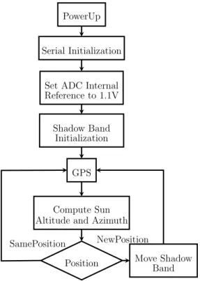
The device was chosen since it is easy to integrate with almost any system, and also because it has the necessary characteristics to perform the control and data acquisition required by the prototype. These characteristics are: size, 6.9cm × 5.3cm; 14 digital in-put/output pins, of which 6 can be used as Pulse Width Modulation outputs; 6 analogue inputs with a 10 bit ADC; USB connection with serial communication between the de-vice and its host; power pins, 5V , 3V 3, Vin and GN D. Figure 4.2 shows the operational

flowchart of the logic module from the moment it is powered up. The main tasks are: Serial Initialization: the serial communication is started at 9600 baud rate, 8 bit, no

(37)

Set ADC Internal Reference to 1.1V : configures the reference voltage used for ana-logue input to 1.1V , by default it is 5V ;

Shadow Band Initialization: this is where the shadow band starts moving from its current position towards bottom, and stops once it activates the dead end switch. Finally the shadow band is moved towards to the 0o position that corresponds to the 0o _{of sun altitude (see Figure 4.9);}

GPS: this routine initializes the GPS module, and retrieves the location coordinates, date and time in GMT ;

Compute Sun Altitude and Azimuth: the sun altitude and the azimuth are com-puted using the GPS data and a sun path algorithm (see subsection 4.4.2.3 for further details);

Position: this is a position check, if the position has changed since the last check then the shadow band moves to the new current position, otherwise it does nothing.

These routines are going to be explained with more detail in the next sections, for further electrical details see Figure A.1.6.

PowerUp

Serial Initialization

Set ADC Internal Reference to 1.1V

Shadow Band Initialization

GPS

Compute Sun Altitude and Azimuth

Move Shadow Band Position

NewPosition SamePosition

(38)

4.4. Cloudiness Indexes

Since cloudiness indexes are based on sky images, the first approach was to take photographs aiming directly at the zenith. However this type of photography can be affected by the extreme brightness of the sun. Therefore, to test the feasibility of this option, a Baxall CDSP9372WF CCTV camera was used (see Appendix A.1.2.1), using a lens without a wide field of view.

Figure 4.3: Shutter speed: 1/10,000; AGC off Figure 4.4: Shutter speed: 1/10,000; AGC on

Figure 4.5: Auto-iris; AGC on Figure 4.6: Auto-iris; AGC off

Changing between the different configuration options, Figures 4.3, 4.4, 4.5 and 4.6 were obtained. Every figure show that despite the glow of the sun, it is possible to have a good perception of what is cloud and what is not. Figures 4.4 and 4.5 are darker than the remaining, which might lead to a sky type classification mismatch in terms of computational analysis. As for the photographs in Figures 4.3 and 4.6, it is possible to see a clear and improved contrast between colours, which eases the image processing determining what is cloud and what is clear sky.

(39)

For this study, the computer system described in Appendix A was used, and two types of implementations were made: one without a shadow band and another using a shadow band that eliminates the reflection on the lens originated by the sun’s flare.

4.4.1 Implementation A: without a shadow band

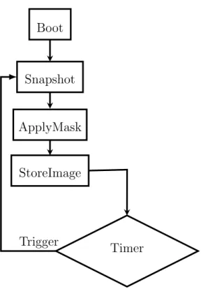
This implementation used the computer setup described in Appendix A. These sky images are taken automatically each minute and one mask is applied to them.

Figure 4.7 illustrates the system operation from booting onwards:

Snapshot: the routine that takes the snapshot of the sky was declared on crontab1 _to

run every minute during the entire year;

Apply Mask: applies an external mask which covers buildings or any other visual inter-ference that affects the components being studied;

Store Image: stores the processed image in a predefined directory, for further analysis;

Timer: triggered every minute, using linux crontab service;

Trigger Snapshot ApplyMask StoreImage Timer Boot

Figure 4.7: Flow chart for implementation A

(40)

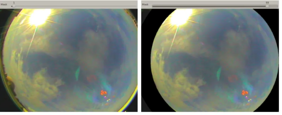
should be positioned in a high location, without taller buildings or other structures nearby, but in urban areas this is quite impossible. This mask allows the user to define the outline for the outer mask of the image, blackening whatever might appear on the image that is not supposed to be classified as clear sky or cloud.

The mask is applied using a software application, where a circle is drawn with a thickness specified by the user (see Figure 4.8). This is done during the setup stage of the system. The user selects the thickness of the circle by moving a slider in the application’s window, which is saved in a file when the application is closed, and used in the sun’s mask algorithm in a production environment.

(a) Before mask definition (b) After mask definition

Figure 4.8: External mask

4.4.1.1 System testing

The implementation was tested mainly on sunny days at noon, to test its behav-ior when exposed to bright light conditions. These conditions were considered as most relevant, since they are one of the types of conditions that lead to many cloud misclassi-fication. Despite the fact that the auto-iris made a difference by reducing the sun’s glow, the lens caused a reflection that can be seen on Figure 4.8. This reflection was not ac-ceptable, since it leads to a misclassification of that part of the image (i.e. clear sky to a cloud). To solve this problem, a shadow band was considered and implemented.

(41)

4.4.2 Implementation B: with a shadow band

This second implementation aims to improve the results obtained using the approach described on section 4.4.1, by adding a shadow band (see Figure 4.9) that follows the sun path position during the day, in order to eliminate the problems caused by the reflection previously mentioned.

Figure 4.9: General view of the shadow band

4.4.2.1 Shadow band

To control the shadow band and its positioning, the following equipment was used: a unipolar stepper motor (see Figure 4.10), N M BP M 55L − 048 − HP 69; an Arduino Duemilanove; a PVC strip to make the shadow band; a CD-ROM belt, to control the shadow band positioning; two plastic discs with 4cm each to couple the shadow band and obtain the desired resolution; and a GlobalSatEM − 406A GPS module (see Figure 4.11) coupled with the Arduino to obtain the geographic location of the system.

The stepper motor used has a full step resolution of 7.5o_{/step, but using a half step}

sequence instead, the resolution is of 3.8o/step. Since the cdrom belt had no teeth, and the teeth of both stepper motor hub and the 4cm disc did not match, its resolution was

(42)

Figure 4.10: Stepper motor

determined using equation 4.1.

Stepper motor resolution = 360

o

number of steps in a turn =

360o

326steps ' 1.1

o _(4.1)

As for the control of the motor and initialization process of the shadow band, it was done using the Arduino. The first action after the system boot is the shadow band initialization. Once the system has power, the band starts moving from north to south until it pushes an end switch. The switch is used to control the initialization process of the band, determining a deference point from where it will start moving. Then the band moves a predetermined number of steps until it reaches de 0o _{position, that is perfectly}

aligned with the zenith, becoming the origin for the upcoming steps.

4.4.2.2 Geographic positioning

The next step of the system initialization depends on the GPS. This is one of the parts that can take more time to initialize, because it has to wait for reliable data from the satellites. Therefore it might take a while depending on the amount of satellites available for connection. The amount of time it takes to connect and retrieve its geographical position and UTC time, depends also on the systems location. It is important to point out, that during tests on our location this procedure was actually very fast.

Once the device is connected and has a fix, the system continues its normal flow. The scheme below, shows the string retrieved from the GPS, and a brief explanation of its fields. The geographic location and UTC time and date, will then be used as inputs to the sun path algorithm.

(43)

Figure 4.11: GPS

GPRMC, 225446, A, 4916.45, N, 12311.12, W, 0.5, 54.7, 191194, 20.3, E *68

1 2 3 4 5 6 7 8 9 10 11 12

1 : UTC time of fix

2 : Data status (A=Valid position, V=navigation receiver warning)

3 : Latitude of fix

4 : N or S of longitude 5 : Longitude of fix

6 : E or W of longitude

7 : Speed over ground in knots

8 : True course

9 : UTC date of fix

10: Magnetic variation degrees (Easterly variation subtracts from true course)

11: E or W of magnetic variation 12: Checksum

(44)

4.4.2.3 Sun path calibration

The sun path calibration was computed using an algorithm based on the study of Carruthers D et al. (1990), which takes as input: time, date, latitude and longitude; and outputs the azimuth, solar declination, solar altitude (in degrees), sunrise time and sunset time. With the calculated data, it is possible to make a stereographic projection of the sun’s path (see Figure 4.12). By plotting this projection on top of a ground sky image with the coordinates perfectly aligned, it becomes possible to see the sun’s path in that specific image.

Analysing Figure 4.12, the vertical axis gives the altitude of the sun. It’s altitude starts on 0o and ends on 90o. The circle represents the angle of the azimuth, its value vary from 0o _{to 360}o_.

Contrary to the system described in chapter 3, the solution to the positioning prob-lem of the prototype depends on both the altitude and the azimuth of the sun.

Figure 4.13 represents the base model used to calibrate the shadow band, it is important to consider that the shadow band is displaced along the yy’s axis, and only moves along the xx’s axis. Figure 4.13 has a representation of the shadow band on the point where the sun is intercepted. On the model, φ represents the altitude of the sun, θ represents the azimuth of the sun,r represents the radius of the shadow band and the black dot represents the point where the sun intercepts the shadow band.

Using the model in Figure 4.13, a conversion from polar to Cartesian coordinates was made, which is represented in Figure 4.14. This represents the triangulation of the three points ABC, which results on the angle (β) that the shadow band has to move to intercept the sun. By computing this angle , the number of steps is computed using equations 4.1 and 4.2