Route planning in wireless sensor networks for data gathering purposes

(1)

UNIVERSIDADE DO ALGARVE

Route Planning in Wireless Sensor Networks for Data

Gathering Purposes

Andriy Mazayev

Master Thesis in Computer Science Engineering

Work done under the supervision of: Profa _{No´elia Correia (FCT/DEEI) e Prof}a_Gabriela Sch¨utz (ISE/DEE)

(2)

Statement of Originality

Route Planning in Wireless Sensor Networks for Data Gathering Purposes Statement of authorship: The work presented in this thesis is, to the best of my knowl-edge and belief, original, except as acknowlknowl-edged in the text. The material has not been submitted, either in whole or in part, for a degree at this or any other university.

Candidate:

——————————— (Andriy Mazayev)

Copyright c Andriy Mazayev. A Universidade do Algarve tem o direito, perpétuo e sem limites geográficos, de arquivar e publicitar este trabalho através de exemplares impressos reproduzidos em papel ou de forma digital, ou por qualquer outro meio conhecido ou que venha a ser inventado, de o divulgar através de repositórios cient´ıficos e de admitir a sua cópia e distribuição com objetivos educacionais ou de investigação, não comerciais, desde que seja dado crédito ao autor e editor.

(3)

NE T W O R K I N G

Work done at Research Center of Electronics Optoelectronics and Telecommunications (CEOT)

(4)

Abstract

Recent studies have shown that mobile elements (ME) in wireless sensor networks (WSN) can drastically reduce energy consumption in such type of networks and thus prolong the sensor network lifetime. Most recent mobile elements used for data gathering are called unmanned aerial vehicle (UAV), commonly known as drones. Although these elements are far faster than terrestrial mobile elements, and used in a wide range of situations, there is a small number of studies on the effectiveness of their use.

In this thesis, after making an analysis of some of the solving methods that might be useful for data gathering, an algorithm is proposed that can provide an efficient use of UAV elements in WSNs. A performance analysis and comparison with existing ap-proaches is done. Results show that the proposed algorithm is able to solve the data gathering problem efficiently presenting, for most data sets and time delivery deadline ranges, a high certainty degree regarding the quality of the solution.

(5)

Resumo

As redes de sensores têm vindo a ganhar importância em vários setores da nossa so-ciedade, sendo a aplicação mais vis´ıvel a monitorização ambiental. Estas redes têm inúmeras aplicações que vão desde a detecção de fogos, medições do n´ıvel de emissões de radiação, detecções de danos estruturais e muito mais, sendo capazes de fazer medições de forma sistemática, e possibilitando desta forma, tomar decisões antecipadas e, assim, evitar acidentes que podem custar vidas humanas.

O envio de dados recolhidos pelos sensores é tradicionalmente feito através de múltiplos saltos (multi hop). Este método baseia-se na passagem dos dados de dispositivo para dis-positivo, através da infraestrutura da rede, permitindo que a informação viage desde a fonte até ao destino graças à passagem dos dados entre elementos vizinhos. Para en-contrar a forma mais eficiente e rápida de fazer chegar a informação ao destino foram propostos, e estão dispon´ıveis na literatura, vários algoritmos que tentam garantir o uso eficaz dos recursos da rede durante o envio dos dados. No entanto, nem mesmo os algo-ritmos mais eficientes são capazes de resolver um problema inerente a esta arquitectura: a entrega dos dados está dependente de vários elementos intermediários. Para além disso, o próprio meio ambiente em que as redes de sensores são utilizadas pode ser um obstáculo durante a comunicação. Poss´ıveis acidentes tais como fogos ou desabamentos podem danificar os canais de comunicação e, desta forma, tornar uma rede de sensores inuti-lizável. As desvantagens presentes na abordagem clássica de recolha de dados levou os investigadores a procurarem outras alternativas.

Estudos recentes têm mostrado que a utilização de elementos móveis em redes de sensores sem fio pode reduzir drasticamente o consumo de energia neste tipo de redes e, assim, prolongar o seu tempo de vida. As abordagens mais recentes no processo de recolha dos dados numa rede de sensores têm reca´ıdo sobre o ve´ıculo aéreo não tripulado, frequentemente conhecido como drone. Embora estes elementos sejam mais velozes do que os elementos móveis terrestres, e devido à sua natureza que permite a sua utilização numa vasta gama de situações, há um pequeno número de estudos sobre a eficácia da sua utilização.

Ao contrário da abordagem multi salto, onde os algoritmos procuram caminhos efi-cientes dentro da própria infraestrutura de rede, a abordagem que envolve elementos móveis necessita de algoritmos que criem caminhos para os próprios elementos móveis. O processo de desenho e criação das rotas é conhecido por problema de recolha de dados

(6)

(Data Gathering Problem). O problema de recolha de dados a ser resolvido nesta tese pode ser descrito como o processo de criação de caminhos para um conjunto de ve´ıculos aéreos não tripulados que têm de recolher dados alojados nos sensores. Terão que ser considerados os seguintes aspectos:

• Janelas temporais de cada sensor. Intervalo de tempo em que o drone tem que visitar o sensor em causa;

• Volume dos dados a serem enviados pelos sensores;

• Tempo de vida útil dos dados. Intervalo de tempo máximo permitido para que a informação seja entregue no destino;

• Conjunto de ve´ıculos aéreos. Cada ve´ıculo aéreo tem a sua capacidade de memória, isto é, limite máximo da quantidade de dados que um drone é capaz de recolher. O processo de criação dos caminhos tem que respeitar todas as restrições temporais dos sensores e, ao mesmo tempo, terá que ser minimizada a distância necessária para recolher os dados de todos os sensores.

A utilização dos ve´ıculos aéreos não tripulados é uma abordagem recente e, talvez por isso, ainda não ganhou a merecida atenção. Como tal, de momento, não existem standards de medição de desempenho de diferentes algoritmos capazes de resolver este tipo de problemas. Nesta tese, tentamos preencher esta lacuna propondo um padrão de medição de desempenho que pode ser utilizado por todos.

São apresentadas duas formalizações matemáticas do problema, uma genérica que pode ser utilizada em vasta gama de situações com semelhantes restrições e uma formaliz-ação estendida que representa o problema a ser resolvido nesta tese. A formalizformaliz-ação genérica permite, identificar este problema com o do encaminhamento de ve´ıculos com janelas temporais (Vehicle Routing Problem with Time Windows).

´

E feita ainda uma análise aprofundada de algumas classes de algoritmos já existentes que podem ser úteis na resolução deste tipo de problemas. Heur´ısticas construtivas, de melhoramento e meta-heur´ısticas são introduzidas e alguns dos seus principais métodos são discutidos. Com base nestes métodos foi desenvolvida uma heur´ıstica h´ıbrida capaz de criar caminhos eficientes não só para o problema recolha de dados numa rede de sensores mas também capaz de resolver o problema de encaminhamento de ve´ıculos. A heur´ıstica apresentada é baseada em três etapas de optimização. A primeira, pré-optimização, que com base nos dados de entrada, cria uma boa solução parcial que será utilizada nos passos seguintes. A segunda fase, designada por optimização, que recebe a solução parcial criada no passo anterior, é responsável pela construção de uma solução inicial que satisfaça todas as restrições de entrada. A última fase, pós-optimização, que recebe como dado de entrada a solução obtida durante a optimização, através de uma combinação de métodos

(7)

tanto determin´ısticos como não determin´ısticos explora de forma eficiente o espaço de procura em busca da melhor solução.

Para medir o desempenho da heur´ıstica h´ıbrida desenvolvida nesta tese foi feito um extensivo conjunto de testes considerando de redes de sensores de várias dimensões, redes com 25, 50, 75 e 100 sensores, e diferentes n´ıveis de restrições temporais. Os resultados obtidos mostram que o algoritmo proposto é capaz de resolver o problema de recolha de dados de forma bastante eficiente apresentando, para a maioria dos conjuntos de dados e para diferentes intervalos de prazos de entrega, um alto grau de certeza relativamente à qualidade da solução.

(8)

Acknowledgements

I would like to thank my parents for their encouragement, education, for their belief in me and for their effort to make my graduation possible. Also, I am grateful to my sister for providing me support during all this time. And finally, I would like to thank my little niece for making my days brighter with her smile.

Special thanks to all my friends that have been by my side since the beginning of this journey. Thanks for your support, all the funny moments that we lived and just for being there for me when I needed it. Without you nothing of this would have been possible.

In academic environment I would like to thank my supervisors, No´elia Correia and Gabriela Sch¨utz. Without their support and guidance I would not have been able to finish this project. Their experience and advices were invaluable.

(9)

1.3.1 Topology Design . . . 4 1.3.2 Network Layer . . . 5 1.4 Problem Definition . . . 6 1.4.1 Practical Applications . . . 7 2 Mathematical Optimization 8 2.1 Introduction . . . 8 2.2 Combinatorial Optimization . . . 8 2.3 NP-Hardness . . . 9 2.4 Mathematical Formulation . . . 10 3 Solving Methods 14 3.1 State Of The Art . . . 14

3.2 Vehicle Routing Problem . . . 15

3.3 Two Step-Algorithm Approaches . . . 15

(10)

3.3.2 Routing Second . . . 16

3.4 Heuristics . . . 18

3.4.1 Constructive Heuristics . . . 18

3.4.2 Nearest Neighbour Heuristic . . . 19

3.4.3 Clarke and Wright Savings Heuristics . . . 19

3.4.4 Push Forward Insertion Heuristic (PFIH) . . . 20

3.5 Improvement Heuristics . . . 22

3.5.1 Ruin and Recreate Principle . . . 22

3.5.2 Local Search . . . 23

3.6 Meta-heuristics . . . 24

3.6.1 Genetic Algorithms . . . 26

3.6.2 Tabu Search . . . 27

3.6.3 Simulated Annealing . . . 28

3.6.4 Multiple Ant Colony Systems (MACS) . . . 29

3.6.5 Guided Local Search . . . 30

4 Data Gathering in WSNs 31 4.1 Introduction . . . 31

4.2 Extended Problem . . . 31

4.2.1 Input and Output . . . 33

4.3 Proposed Hybrid Heuristic Algorithm . . . 34

4.3.1 Problem Limits . . . 34

4.3.2 Adapted Push Forward Insertion Heuristic . . . 34

4.3.3 Seeded Partial Solution . . . 35

4.3.4 Improvement Methods . . . 36

4.3.5 Node Ejection . . . 38

4.3.6 Band Neighbourhood Ejection . . . 39

4.3.7 Overall Procedure . . . 40

5 Performance evaluation 43 5.1 Introduction . . . 43

5.2 Data Set and Best Known results . . . 43

5.2.1 Generating Data Sets . . . 43

5.2.2 Best Known Results . . . 44

5.3 Getting the Results . . . 45

5.3.1 Heuristic Results . . . 45

5.3.2 Exact Results . . . 45

5.4 Analysis of the Results . . . 46 5.4.1 Optimal vs Heuristic Solutions for Sets C1 and C2 with 25 Nodes 46

(11)

5.4.2 Heuristic Solutions for all Sets with 25 Nodes . . . 48 5.4.3 Best known vs Heuristic results with 100 Nodes . . . 51

6 Conclusion and Future Work 54

6.1 Conclusion . . . 54 6.2 Future Work . . . 54

(12)

List of Figures

1.1 Choke point. . . 6

1.2 Problem illustration. . . 7

2.1 Graph representation. . . 10

3.1 Example of a problem before clustering process. . . 16

3.2 Example of a problem after clustering. . . 17

3.3 Example of a problem solution. . . 17

3.4 Solution produced by constructive heuristic. . . 18

3.5 Example of route merging between node i and j. . . 20

3.6 Solution produced by improvement heuristics. . . 23

3.7 Intra route operators (Cari´c et al., 2008). . . 24

3.8 Inter route operators (Cari´c et al., 2008). . . 25

3.9 Solution produced by meta-heuristic. . . 26

3.10 Entropy rate. . . 28

3.11 Multiple ant colony systems Gambardella et al. (1999). . . 29

4.1 Seeded partial solution. . . 36

4.2 Solution representation . . . 37

4.3 2-Opt operator. . . 37

4.4 Crossover operator. . . 38

4.5 Band neighbourhood ejection. . . 40

5.1 Average distance increase factor. . . 49

5.2 Lowest distance increase factor. . . 49

5.3 Highest distance increase factor. . . 50

5.4 Average number of UAVs increase factor. . . 50

5.5 Lowest number of UAVs increase factor. . . 51

(13)

List of Tables

1.1 Comparison between different data gathering approaches. . . 4

2.1 Solutions for perimeter minimization. . . 9

5.1 Heuristic’s performance for delivery limit equal to ∆3 and ∆4 . . . 47

5.2 Heuristic’s performance for delivery limit equal to ∆5 and ∆6 . . . 48

5.3 Results obtained with the proposed method for instances with infinite de-livery limit of the Solomon’s benchmark with 100 nodes. . . 53 A.1 Adapted Solomon instances with 25 nodes . . . A-2 A.2 Adapted Solomon instances with 50 nodes . . . A-3 A.3 Adapted Solomon instances with 75 nodes . . . A-4 A.4 Adapted Solomon instances with 100 nodes . . . A-5

(14)

List of Algorithms

1 Nearest neighbour heuristic. . . 19

2 Clarke and Wright savings heuristic. . . 21

3 Push forward insertion heuristic. . . 22

4 Local search. . . 25

5 Genetic algorithm. . . 26

6 Tabu search. . . 28

7 Simulated annealing. . . 29

8 Seeded partial solution. . . 35

9 Band neighbourhood ejection. . . 39

(15)

List of Publications

1. Pedro J.S. Cardoso, Gabriela Sch¨utz, Andriy Mazayev, Emanuel Ey, ”Solutions in under 10 seconds for vehicle routing problems with time windows using com-modity computers”, 8th International Conference on Evolutionary Multi-Criterion Optimization, EMO 2015; Guimar˜aes, Portugal, 29 March – 1 April 2015.

2. Pedro J.S. Cardoso, Gabriela Schütz, Jorge Semião, Jânio Monteiro, João Ro-drigues, Andriy Mazayev, Emanuel Ey, Micael Viegas, Carlos Neves, Sérgio Anastácio, ”Integration of a food distribution routing optimization software with an enterprise resource planner”, International Conference on Geographical Information Systems Theory, Applications and Management, Barcelona, Spain, 28-30 April, 2015. 3. Pedro J. S. Cardoso, Gabriela Schütz, Andriy Mazayev, Emanuel Ey, Tiago Corrêa,

”A Solution for a Real-time Stochastic Capacitated Vehicle Routing Problem with Time Windows”, 15th International Conference on Computational Science, Reyk-jav´ık, Iceland, 1–13 June (accepted).

4. Andriy Mazayev, No´elia Correia, Gabriela Sch¨utz, ”Heuristic Approach for Data Gathering in Wireless Sensor Networks”, IEEE International Conference on Com-munications, London, United Kingdom, 8–12 June (accepted).

(16)

C H A P T E R

1

Introduction

1.1 Background

Sensor networks are ad-hoc networks composed of sensors that are connected wirelessly. The main goal of sensors it to capture the state of the environment (temperature, humidity, luminosity, etc.) and to relay this information to an entity (sink node or base station) more suited for data processing, visualization, analysis and decision making upon the informa-tion received. A sensor node, also called node, is a small sensing capable device with limited processing capability, reduced memory capacity and bandwidth, and a limited source of energy (Rodrigues and Neves, 2010). Despite of all these hardware limitations, sensors are very useful nowadays. They are cheap, small in size, easy to install and highly flexible. This allows them to be used in a high range of situations, from simple luminosity measurements to radiation measurements in atomic plants (Chin et al., 2010).

Since sensor nodes are limited in processing capabilities, local data analysis may not be a viable option and, therefore, it becomes crucial to forward the data to a device with higher capabilities for further processing. Usually this is done by the network infrastruc-ture itself without any third part involved in this operation. This type of data forwarding is called multi-hop and it involves one or more nodes to forward the data from a sensor to a sink node. In such cases, a power consumption problem arises. In order to send the data from one point to another, other nodes must first receive the information and then forward it, even without having anything do to with the data itself. It is known that, in sensors net-works, the transmission process is the one spending more energy. Hence, the lifetime of a network is reduced if data is simply forwarded with no energy concern in mind. Replac-ing the energy source of a sensor may not be viable because of the surroundReplac-ing conditions where the sensors are installed (atomic plant, underground, etc.). In most cases once the sensor is discharged there is nothing left to be done. All these constraints mean that data transmission must be thoughtful and must be used only when necessary in order to extend network operation.

Another and more recent approach to gather the data in sensor networks involves mo-bile elements. By moving directly to the source, receiving the information directly from

(17)

1.2 Data Gathering Approaches

it and then delivering it to the destination, mobile elements allow multi-hop communica-tion, which is energetically inefficient, to be avoided and thus the lifespan of a network to be extended. A mobile element can be of terrestrial type, travelling over the land, or an aerial element, called unmanned aerial vehicle (UAV).

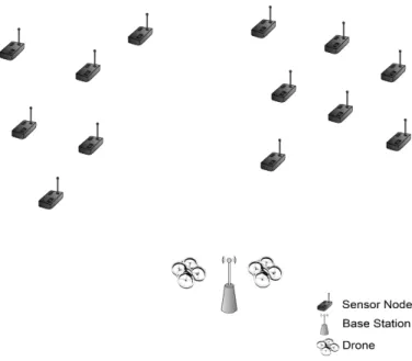
This thesis focus on data gathering in WSNs using elements of UAV type. The goal is to develop an algorithm that can design a set of efficient paths to gather the data generated by sensor nodes, which are scattered over a given area. More specifically, the contribu-tions of this thesis are:

• A mathematical formalization of the data gathering problem is presented;

• A deep analysis of the existing solving methods, useful in these kind of problems, is done;

• A hybrid heuristic algorithm is proposed;

• A standardized benchmark is introduced to measure the performance of the pro-posed algorithm;

• A head-to-head comparison between the results obtained by the proposed algorithm and the optimal solutions is done

1.2 Data Gathering Approaches

As stated earlier there are two approaches to gather the information in a sensor network. Each of these has it own pros and cons that will be discussed in the following subsections.

1.2.1 Classical Networks

In classical networks the data is transferred through the network infrastructure itself from the sensor node to the base station. Due to energy concerns the throughput in a sensor network is very limited, normally reaching only a few Kbps. Transmission is the most energy demanding task that sensor nodes perform. This means that any communication, and specially multi-hop communication, must be avoided and used only when it is strictly necessary to maintain network operation for a long time. The main advantage of this approach is the small delay on data delivery, which can reach a few seconds or even less.

1.2.2 Networks with Terrestrial Elements

In this approach mobile robots are used to collect the data from sensors for a later delivery to a base station for further processing. In this case bandwidth is higher, capable to achieve

(18)

1.3 Network Design Problems in Sensor Networks

few Mbps. The most prominent issue with this approach is a time delay between receiving the data from all sources and delivering it to destination. Since the travelling speed of terrestrial elements is considerably low, in most cases inferior to one meter per second (Tekdas et al., 2009) (Richard Pon, 2005) the delay between sensing the data at the sensor and processing it at the base station is significant. It may take several hours to gather all the data and deliver it to a base station.

Similarly to the previous approach a power consumption problem also arises. Power consumption at mobile elements is very high since mobile elements may have consider-able size and must visit all the nodes to gather the information. However, in this case, replenishing the power source of the mobile element is not a problem since it is easily accessible. This approach can fully eliminate multi-hop communication at the expense of delay.

1.2.3 Network with UAV Elements

A UAV approach is in all similar to the approach stated above. The main advantage in this case is the drastic reduction of the delay. Since we are talking about an element with fly-ing capabilities its travellfly-ing speed is much higher than terrestrial elements. Therefore, it can collect data scattered across all the sensors much more efficiently and quickly. Some research has been done on the use of UAVs in WNS (Sujit et al., 2013), (Pignaton de Fre-itas et al., 2010), (Costa et al., 2012). However, the UAV approach has still not reached the deserved attention.

Performance metrics Multi-Hop Terrestrial Element UAV

Delay Low (second) High (hours) Medium (minutes)

Energy Consumption High

(non rechargeable) High (rechargeable) High (rechargeable) Bandwidth Medium (few Kbps) Medium-High (few Mbps) Medium-High (few Mbps)

Table 1.1: Comparison between different data gathering approaches.

1.3 Network Design Problems in Sensor Networks

1.3.1 Topology Design

Designing an efficient sensor network may be a problem by itself. How to know where to put the sensors in order to achieve a good performing network? What to do if sensor nodes are scattered or randomly placed? The physical distribution of nodes can be a difficult

(19)

1.3 Network Design Problems in Sensor Networks

task by itself. In case of random sensor distribution there is no guaranty whatsoever that multi-hop based protocols will work. Some of the sensor nodes may be out of range of the network thus compromising its quality. A network should always be carefully designed and optimized in order to work properly, which usually involves environment analysis and studies. Different topologies have been proposed to maintain the reliability of the sensor network (Mamun, 2012). In a star topology the sensor nodes maintain a direct communication line with the base station. This basic approach is suitable for simple cases. However, due to direct communication limitation this topology in not capable to cover extensive areas and requires predetermined positioning of nodes. A tree topology is capable to solve this coverage issue. As in a star topology, each node has a single communication path toward the base station but in this case other nodes can act like forwarding elements and thus the covered area is extended. However, the topology is not fault tolerant because if a single routing node fails the sensor nodes will lose their communication path toward the base station. The mesh topologies, by adding redundant communication paths, remediate the reliability issues of tree topologies at the expense of additional hardware.

The use of mobile elements that can go directly to a source and gather the information could greatly relief the process of topology design because of routing flexibility.

1.3.2 Network Layer

Even if the topology is well designed there are still issues with sensor networks. How to correctly disseminate the data? How to efficiently forward data provenient from another node? The layer responsible for creation of paths between a source and a destination is called network layer. This layer is strongly influences the efficient use of network infrastructure. The process of data delivery through the network is called routing. In case of predetermined node distribution it is possible to create delivery paths a priori. However, in a random distribution that can result in non uniform topologies the sensors must be able to determine their positions, discover their neighbours and identify paths to a base station, which can be a difficult task.

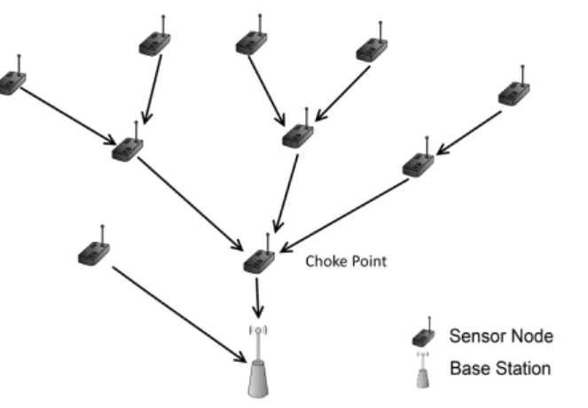
Another critical issue in wireless sensor networks are choke points (Figure 1.1). As shown in Figure 1.1 a sensor node where choking occurs not only has to send its own data to a base station but also has to forward the data from many other nodes. As a result the power consumption of this node will be extremely high and it will deplete its power source much quicker than the other sensor nodes. When this occurs the network becomes unusable since the information does not reach its destination. Moreover, if a sensor network is composed of sensor nodes of different types and different sampling rates then network traffic becomes unbalanced resulting in performance inefficiency. Paths must be designed in a balanced way in order to extend the life span of a network. To solve

(20)

1.4 Problem Definition

Figure 1.1: Choke point.

the issue presented in Figure 1.1 traffic could be split between two sensors nodes that are in the vicinity of the base station.

Another approach to deliver the data can be achieved with a mobile element. In this case, instead of designing paths for a multi-hop communication, the paths are designed for the mobile element itself. This way, the mobile element travels throughout all the network in an efficient way and gathers all the information directly from the source before delivering it to a base station. An optimization of paths is a crucial point of a good performing sensor network.

After exposing all these issues it is now possible to generally describe the problem to be solved in this thesis.

1.4 Problem Definition

Given a set of nodes distributed on a surface with respective coordinates and their time restrictions, given a sink node with its own coordinates and also a set of UAVs that can freely travel over the surface, the goal is to create paths in such a way that:

• All node are visited only once

• All routes begin and end at the sink node • All time restrictions are respected

• The number of mobile elements is kept minimum during the data gathering process • Total travelling distance is minimized

In this thesis it is assumed that the distance between any pair of nodes can be given by the euclidean distance, which may not be possible in reality but since we are trying to make a theoretical demonstration euclidean distance will suffice. Also, the distribution of

(21)

1.4 Problem Definition

Figure 1.2: Problem illustration.

nodes may be random (R), clustered (C) or both random and clustered (RC). Finally, each sensor nodes has its own unique time restrictions.

The problem described in this section is NP-hard. A more detailed description of this implication will be done in Chapter 2.

1.4.1 Practical Applications

Due to the existence of some delay when using mobile elements the approach presented in this thesis should not be used in critical situations, such as fire, radiation, structural damage monitorization and detection when it is required response at the time. In these cases every second counts and, therefore, the classical multi-hop approach is preferable. However, even in these cases, due to structural damage and possible disruptions in com-munication channels drones may become handy as they do not require additional infras-tructure to gather the data. In other cases where the delay is not an important aspect mobile elements can and should be used.

At the research center where this thesis was developed, this problem, is expected to be applied, in the future, to detect the cork tree decease at an early stage. This project is just starting at the Center of Electronics Optoelectronics and Telecommunications (CEOT) and is currently in an early development stage.

The UAV approach can also be used to forecast eventual wildfire occurrences and to warn about the necessity to perform prevention measures. In order to accomplish this it is necessary to place temperature, humidity and wind sensors over the area being mon-itorized and periodically gather the data from them. In Portugal, especially during the summer, the wildfire is a common event and monitorization could reduce drastically the number of fire incidents.

(22)

C H A P T E R

2

Mathematical Optimization

2.1 Introduction

Mathematical optimization is a field of mathematics whose goal, depending of the prob-lem to be solved, is to minimize or maximize the value of the objective function through the combination of feasible variables. Generally, a mathematical optimization can be described in the following way:

minx∈Sf (x) (2.1)

where:

• f (x) is the objective function;

• S is the set of feasible values that x can take; • x, depending of the problem, can be integer or real.

The expression 2.1 means that variable x can only take values of set A and for each of these values the objective function gives a quantitative description about the solution. In this case in particular, the goal is to find x in such way that the f (x) is minimum.

The duality theorem allows to rewrite the function 2.1 as maximization problem. However, since we are tackling a cost minimization problem, the remaining part of this report will only focus on minimization functions.

2.2 Combinatorial Optimization

Combinatorial optimization is one of the branches of the mathematical optimization. Likewise the mathematical optimization, the goal is to minimize the cost of the objective function. However, in combinatorial optimization the variables are discrete and belong to a finite set.

(23)

2.3 NP-Hardness

For a better understanding of the combinatorial optimization concept let us take a look at a simple example.

Minimize the perimeter of a square in such a way that the product of length and width is equal to 10.

min2x + 2y (2.2)

subject to:

xy = 10 (2.3)

x, y ∈ N (2.4)

Table 2.2 presents the set of possible solutions for the problem stated above. Solution x y Perimeter

1 1 10 22

2 2 5 14

3 10 1 22

4 5 2 14

Table 2.1: Solutions for perimeter minimization.

As shown in Table 2.2, all solutions are feasible since all of them satisfy the con-straints. However, only solution 2 and 4 minimize the perimeter and thus only these two solutions suit this problem.

2.3 NP-Hardness

Routing and scheduling problems complexity have been largely explored and studied and it has been consistently proven that routing problems are NP-hard. NP problems are not solvable in polynomial time O(nk) where n is the input size of a problem and k is some constant. In fact, NP class consists of a set of problems whose solution can be efficiently verified but finding the actual solution is a quite difficult task.

The fact that the problem studied in this thesis is NP-hard implies that alternative ap-proaches are required to solve it, namely heuristic methods. A more detailed explanation about routing and scheduling problems complexity can be found in (Lenstra and Kan, 1981).

(24)

2.4 Mathematical Formulation

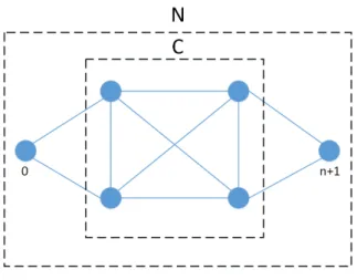
A generic data gathering problem consists in collecting the data of a set of nodes using a set of UAVs. The problem can be represented by a graph G = {N, A} where N = {0, 1, . . . , n, n + 1} is a set of vertices, A ⊂ {(i, j) : i, j ∈ N } is a set of edges and C = N \ {0, n + 1} is the set of sensor nodes (Ombuki et al., 2006).

Figure 2.1: Graph representation.

Nodes 0 e n + 1 represent the base station, starting and ending points for all UAV’s paths. The remaining nodes 1, 2, ..., n represent the sensor nodes that must be visited. If in a real case the starting and ending points are the same then node n + 1 can be seen as a virtual node for formulation purposes. The set of edges of a graph, represented by A, contains all possible link between all the nodes, including the base station, of the problem. In this case in particular it is assumed that the graph is complete, i.e., it is possible to travel from a node ni ∈ N to any other node from nj ∈ N \ ni

Each edge has its own cost cij and a time tij, (i, j) ∈ A. The cost cij represents the cost associated to a travel between the vertex i and vertex j. Similarly, tij represents the time required to travel from vertex i to vertex j. In this case, and for theoretical purposes, it is assumed that the cij = tij = dijwhere dij is the euclidean distance between vertices i and j. But the developed algorithm is generic and can perform optimization even in cases where the equality is not met.

The set of UAVs is denoted by V and each UAV v ∈ V has it own buffer size qv. Each sensor node n, represented by a vertex at the graph, has data dnto be gathered, n ∈ C. Each sensor node n can have a time window [stn, etn], where stn and etn represent the start time and end time of a sensor node, respectively. An UAV can arrive to a node n before its start time but it will have to wait until sti to receive the data. In the other hand, an UAV is not allowed to arrive to a node n after end time etn.

All UAVs must start at the base station within the range [st0, et0] and arrive to a base station within [stn+1, etn+1]. These intervals represent time windows of a base station.

(25)

In this particular case, the start time restriction is irrelevant because base stations are, normally, always active and we can assume that st0 = 0, i.e., all routes start at instant 0. However, to design a generic algorithm that could operate even in cases when a base station has other time windows, this restriction should be taken into account.

The model described results in a problem with three decision variables, x, v and a. For each edge (i, j), where i 6= j, i 6= n + 1, j 6= 0, and for each UAV v, the decision variable xijv is equal to 1 if UAV v travels from node i to node j, 0 otherwise. The decision variable aiv represents the arrival time of UAV v ∈ V to node i, i ∈ C. The decision variable ϑv is equal to 1 if current UAV is required to gather the data, 0 otherwise.

The goal of the gathering problem is to gather the data from nodes C by using UAVs from V in a way that the distance during the gathering process is minimized. This con-straint can be expressed using a cost function because smaller distance implies smaller costs. However, these requirements must comply with the following constraints:

• Buffer size of UAV • Time windows

• Each node must be visited only once

• All routes begin at node 0 and end at the node n + 1 The problem is formulated as follows:

minX v∈V X i∈N \{n+1} X j∈N \{0} cijxijv (2.5) Subject to: X v∈V X j∈N \{0} xijv = 1, ∀i ∈ C (2.6) X v∈V X i∈N \{n+1} xijv = 1, ∀j ∈ C (2.7) X i,j∈sXs xijv ≤ |S| − 1, ∀v ∈ V, S ⊆ {1, ..., n} , 2 ≤ |S| ≤ n − 1 (2.8) X i∈C di X j∈N \{0} xijv < qv, ∀v ∈ V (2.9) X j∈N \{0} x0jv = ϑv, ∀v ∈ V (2.10) X i∈N \{n+1} xihv− X j∈N \{0} xhjv = 0, ∀v ∈ V, ∀h ∈ C (2.11)

(26)

2.4 Mathematical Formulation X i∈N \{n+1} xi,n+1,v = ϑv, ∀v ∈ V (2.12) a0v = 0, ∀v ∈ V (2.13) aiv+ si+ tij − K(1 − xijv) ≤ ajv, ∀v ∈ V, ∀i ∈ N \ {n + 1} , ∀j ∈ N \ {0} , i 6= j (2.14) ϑvsti ≤ aiv≤ ϑveti, ∀v ∈ V, ∀i ∈ N (2.15) xijv ∈ {0, 1}, ϑv ∈ {0, 1}, aiv≥ 0, ∀v ∈ V, ∀i ∈ N, ∀j ∈ N (2.16) Where: Sets V = {1, 2, ..., v} set of UAVs

N = {0, 1, ..., n, n + 1} set of nodes including the base station

C = {1, 2, ..., n} set of nodes

A = {(i1, j1) : i, j ∈ N, i 6= j} set of edges

Constants

di amount of data to be gathered

at node i ∈ N

sti start of the time window

of node i ∈ N

eti end of the time window

of node i ∈ N

qv buffer size of UAV v ∈ V

cij cost of travelling from node i

to j, i, j ∈ N

tij travel time from node i

to j, i, j ∈ N

si service time at node i ∈ C

K is a large value

Decision variables

xijv one if UAV v ∈ V

travels from node i to node j, i, j ∈ N

aiv arrival time of UAV v ∈ V

to node i ∈ N

ϑv one if vehicle v ∈ V

is required to gather the data The objective function (2.5) indicates that the costs must be minimized. Constraints (2.6) and (2.7) indicate that each node must be visited by a single UAV. Constraints (2.8)

(27)

avoid the formation of subcircuits. Constraints (2.9) indicate that buffer size of the UAV v can not be exceeded. Constraints (2.10), (2.11) and (2.12) are flow restrictions. The first one (2.10) indicates that all UAVs must start at the base station, the second one (2.11) indicate that UAV can not stay at the node, i.e., the UAV must arrive to a node, gather the data and depart. Constraints (2.12) indicate that paths must end at the base station. Constraints (2.13) indicate that all UAVs start gathering process at instant zero. Constraints (2.14) indicate that UAV v can not arrive at node j before aiv+ si+ tij if it travels from node i to node j. Constraints (2.15) state that time window restriction must be met. Finally, the (2.16) restrictions define variables.

Note that this formalization can be applied to many gathering problems. In the fol-lowing sections this will be adapted to the data gathering problem in WSNs using UAVs, where data collected can also have a period of validity (Time-To-Live), which is not in-cluded in this formalization.

(28)

C H A P T E R

3

Solving Methods

Most of the research on data gathering in WSNs uses adaptations or variations of the Ve-hicle Routing Problem (VRP) that was and continues to be a hot topic in the optimization field. The main reason is attached to economic grounds. More and more transport com-panies are embracing software utilities which can improve their business models in many aspects such as cost reduction and more efficient use of resources during the distribution and/or gathering of the goods. Another but not less important reason is the inexistence of a good performing algorithm which could solve all routing problems seamlessly. This simple fact draws the attention of researchers from all over the globe.

Mobile element routing have not draw much attention in academic field. As result, when compared with other optimization problems, such as the VRP, mobile element rout-ing is just a drop in an ocean. Due to little research about mobile element routrout-ing in WSNs and due to its similarity with the VRP we will gather knowledge about solving methods in a known and largely studied area and adapt them to the mobile element routing.

3.1 State Of The Art

In this section we will take a look at some of the mobile element routing problems tackled by researchers.

In Data Gathering problem (Bhadauria and Isler, 2009) all sensor nodes must be vis-ited in such way that the expended time to perform this task is minimum. This problem is a variation of k-Travel Salesman Problem.

Time-constrained Mobile Element Scheduling (Almi’ani et al., 2010) state that all sensor nodes must be visited within their own time window, i.e., period of time when sen-sor is awake and capable to communicate. This problem is a straightforward adaptation of VRP-TW in a sensor network.

In Deadline Scheduling (Somasundara et al., 2007) a set of sensor nodes with limited buffer size and different sampling rate must be visited before their buffer overflows. In Calibration Scheduling (Bychkovskiy et al., 2003) sensor nodes must be visited and cali-brated before the error of sensed data exceeds a certain threshold. These problem can also

(29)

3.2 Vehicle Routing Problem

be viewed as VRP-TW where the deadline to visit a node represents a time window. In Rendezvous Planning (Xing et al., 2008) there are intermediate buffer nodes (ren-dezvous points) where the data from the sensor nodes is stored. In this problem the data generated by sensors must be delivered to a base station within a certain deadline. The delivery is done by mobile elements that travel to rendezvous points to gather the data and deliver it to destination. This problem can be viewed as simplified VRP-PD (Pickup and Delivery) where the data must be picked up at rendezvous points and delivered to the destination.

As seen, all these are adaptations of VRP. Therefore we will take a close look at the original problem and its solving methods and then apply them to a WSN with mobile elements problem.

3.2 Vehicle Routing Problem

In the VRP the goal is to find the best set of routes to visit all the clients distributed across a certain geographical area. However, in order to understand this definition it is necessary to define clearly what is the ”best route”. Best route is one that results in a minimum usage of resources without violating any of restrictions imposed by the problem. Usually VRP has time and capacity restrictions.

• Time Restriction (Time Windows) - the vehicle must visit the clients in a time win-dow defined by clients. Time winwin-dows can correspond to a normal working day. For example, let us assume that there is a client with the following time window -from 9 a.m. until 5 p.m.. This means that the distribution vehicle is obliged to visit and serve this client during this time window. In case of a mobile element routing in sensor networks this could correspond to a state when the sensor is in awake mode and is performing some activity. Similarly to a vehicle in VRP, the UAV must visit a sensor when it is active and has some data to send, or due to a deadline to visit a node with a limited buffer size.

• Restriction Capabilities (Capacitated Problem) - this restriction limits the number of visiting clients. A vehicle can not serve a client if it does not have the capacity to transport the required goods. In sensor networks with mobile elements this could correspond to data to be gathered by the UAV. An UAV can not visit and gather the data of a sensor node if its buffer does not have the capacity to receive the data.

3.3 Two Step-Algorithm Approaches

By nature, the human being has difficulty to process large quantities of information. Usu-ally this task is done through the decomposition of the data into smaller and independent

(30)

3.3 Two Step-Algorithm Approaches

parts followed by processing and analysis of those parts. This strategy is called divide-and-conquer. The division step implies the decomposition of a problem in small parts and conquer stands for a resolution of decomposed parts which, when combined, result in a solution to the original problem. This simple method has large applications in science, and computer science is no exception, not even the most powerful computers are able to solve, in a reasonable time, optimization problems with extremely large number of vari-ables. In order to accelerate the search for the solution a two step algorithm can be used, Cluster First - Route Second.

3.3.1 Clustering First

Clustering is done in the initial phase, before solving the problem. At this stage all nodes (clients or sensor nodes) are equal and belong to a single set (Figure 3.1).

Figure 3.1: Example of a problem before clustering process.

The clustering process is done according to some criteria, normally by geographical localization but it also could be done following any other criteria that can allow the cluster formation based on the similarity features of the nodes (Figure 3.2).

Upon the completion of clustering stage, the original problem is decomposed in a set of independent sub-problems with a smaller size and easier to solve. Normally, each cluster can be seen as a travelling salesman problem (TSP) (Baker, 1983) to which time windows restrictions can be added.

3.3.2 Routing Second

Once the clustering is complete and the problem is divided, each of the clusters can be separately solved. For each cluster, a mobile element or a set of mobile elements will

(31)

3.3 Two Step-Algorithm Approaches

Figure 3.2: Example of a problem after clustering.

be assigned. They will be responsible for the data collection from their cluster (Figure 3.3). During this step a numerous amount of methods can be applied, exact approaches or heuristic and meta-heuristics.

Figure 3.3: Example of a problem solution.

The two step algorithm facilitates the search of the solutions as it divides the prob-lem in a set of independent sub-probprob-lems. The division of the original probprob-lem reduces drastically the search space, which consequently results in a more efficient search of the solution for the original problem.

(32)

3.4 Heuristics

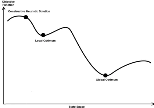
Heuristics are a set of algorithmic methods whose goal is to find the optimum solution for an optimization problem. These methods have a certain degree of ”knowledge” about the problem, which allows them to perform a relatively small search in the search space. Usually heuristics are capable to generate acceptable solutions in short periods of time.

However, it is important to mention that there is no guarantee that the solution found is optimum or even if it is near it. The only way to evaluate the quality of the generated solution is to solve the problem and find the optimum solution but, as seen earlier in Chapter 2.3, this is a difficult task.

3.4.1 Constructive Heuristics

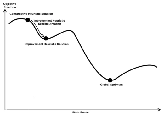
Constructive heuristics build the solution in an iterative way. These heuristics start with an empty solution and at each iteration the current solution is extended. This process is repeated until the complete solution is constructed. Usually constructive heuristics are greedy and do not possess backtracking mechanics, i.e., once an element is inserted in the solution it is impossible to remove it.

Figure 3.4: Solution produced by constructive heuristic.

Figure 3.4 is an example of what a constructive heuristic can produce. As shown, the solution generated can be far from optimum and could offer a lot of space for improve-ments. Improvements that can be done by other set of heuristics, which will be addressed in Chapter 3.5.

(33)

3.4 Heuristics

3.4.2 Nearest Neighbour Heuristic

Nearest neighbour heuristic is probably the most intuitive and, perhaps because of that, it is the easiest to understand. As the name suggests, the idea behind this algorithm is to choose always the closest node to the current position of the mobile element. However, a possible time restriction must be taken into account, meaning that choosing the closest node is not a straightforward process. In order to find the closest neighbour the following cost function can be used (Jaheruddin, 2010):

cij = δ1dij + δ2tij + δ3vij (3.1) Where:

• cij travelling cost between node i and j • dij distance between node i and j

• tij time difference between completing node i and staring node j • vij remaining time until last possible start of j following i • δ1+ δ2+ δ3 = 1 and δ1 ≥ 0, δ2 ≥ 0, δ3 ≥ 0

The nearest neighbour heuristic can be described in a generic way by Algorithm 1. Algorithm 1: Nearest neighbour heuristic.

input : G = (N , A) and set of UAVs V. output: Feasible solution

1 Start with first mobile element at the base station 2 while there are nodes to be visited do

3 while mobile element is not full or there are nodes to visit do 4 Find closest and unvisited node to current node

5 Assign closest node to the current mobile element

6 end

7 Choose next mobile element 8 end

3.4.3 Clarke and Wright Savings Heuristics

The main concept of this method is to reduce costs by merging two or more routes in a single one (Florˆencio, 2011). However route merging must comply to all the restrictions imposed by the problem being solved.

(34)

3.4 Heuristics

Figure 3.5: Example of route merging between node i and j.

The economy of resources by route merging can be quantified by a mathematical formula. For a better understanding of the formula let us apply it to Figure 3.5. In case (a) the travelling cost can be expressed in a following way:

da = c0i+ ci0+ c0j + cj0 (3.2)

Where cab is the cost of travelling from node a to a node b. Similarly for case (b):

db = c0i+ cij + cj0 (3.3)

The amount of saved resources is given by the difference between the resources used in case (a) and in case (b)

Sij = da− db = ci0+ c0j − cij (3.4) However, before merging the two paths it is necessary to check if the resulting route will be able to satisfy all the restrictions imposed by the problem. There are cases where one route can be merged with two or more other routes. In this case, the tie is broken by the value of Sij, route with the highest value of Sijis chosen, as the goal is to minimize the costs. A generic description of Clarke and Wright savings heuristic is done in Algorithm 2.

The Clarke and Wright algorithm has two variations, the sequential one and parallel one. In the parallel version multiple routes are built simultaneously. Usually, the parallel version produces sightly better results.

3.4.4 Push Forward Insertion Heuristic (PFIH)

Push forward insertion heuristic (PFIH) is a greedy heuristic presented by Solomon (1987). This method has been implemented and tested by several authors (Thangiah et al., 1993), (Russell, 1995), (Thangiah, 1999), (Tan et al., 2001). The operational sequence of this algorithm is quite simple. First step is to classify and define the sequence by which nodes will be inserted in the solution. Usually, this is done by the following cost function

(35)

3.4 Heuristics

Algorithm 2: Clarke and Wright savings heuristic. input : G = (N , A) and set of UAVs V.

output: Feasible solution

1 Create a direct route for each node 2 while cost saving merge exists do 3 Choose a route

4 Compute all possible cost saving merges for current route 5 Sort all merges by S_ij

6 while current route is mergeable do

7 if merge does not violate restrictions then

8 Merge routes 9 end 10 end 11 Next route 12 end Thangiah et al. (1994): ci = −α × di,0+ β × eti+ γ((pi/360) × di,0) (3.5) Where:

• ciPFIH cost of node i.

• di,0 distance between node i and base station. • eti upper limit of time window of node i.

• pipolar angle between node i and the base station. • α + β + γ = 1

Different α, β and γ values can be used to give more or less importance to formula parcels, resulting in distinct ordering of the nodes. For instance, large values of α will make more preferable nodes farther from the depot. Larger values of β will make nodes with earlier closing window preferable. Larger values of γ will make preferable to insert the nodes in a circular spanning mechanism (like a ”radar”). Normally, α is set to 0.7, β to 0.1 and γ to 0.2. However, these values were empirically established by Thangiah et al. (1994), Ghoseiri and Ghannadpour (2009) and other values can be used. Given the cost of all nodes, insertion is quite straightforward (Algorithm 3).

Usually this method is used to establish the upper bound of the problem. The solution produced by this heuristic is mostly used as input information in other methods for further improvements.

(36)

3.5 Improvement Heuristics

Algorithm 3: Push forward insertion heuristic. input : G = (N , A) and set of UAVs V. output: Feasible solution

1 Calculate PFIH cost for each node 2 Sort all the nodes by their PFIH cost 3 while there are nodes to be visited do 4 if number of routes != 0 then

5 Insert in the route where the insertion causes minimal distance increase 6 if not possible then

7 Create new route

8 Insert current node into recently created route

9 end

10

11 else

12 Create new route

13 Insert current node into recently created route

14 end

15 16 end

3.5 Improvement Heuristics

Unlike constructive heuristics that start with an empty solution and build a new solution in an iterative way, improvement heuristics start with an already existing and feasible solution. At each iteration the improvement heuristic explores the neighbourhood of the current solution to find a better one.

The main problem with this process and with all improvement methods in general is that they do not possess mechanisms to escape local optimums. When a local optimum is found, the algorithm enters in a stagnation stage, i.e, all neighbours are worse than the current solution and no further improvement is possible. Figure 3.6 represents the search direction of the improvement heuristic, the sequence of the explored neighbours and the solution produced by it.

In this example the improvement heuristic received as input the solution produced in Figure 3.4.

3.5.1 Ruin and Recreate Principle

Since the constructive heuristics are usually greedy methods, i.e., at each iteration the decision is made by a local criteria, the final solution may be far from optimum. Hence solutions produced by constructive heuristics offer room for improvements most of the times. The ruin and recreate principle (Schrimpf et al., 2000) is a two step improvement method that can be used to improve current solution. During the first stage of this method

(37)

3.5 Improvement Heuristics

Figure 3.6: Solution produced by improvement heuristics.

a set of nodes is ejected from the solution. There are many criteria to eject a set of nodes: • Random ejection - from each route a random number of nodes is ejected;

• PFIH cost based ejection (obtained after execution of PFIH (Chapter 3.4.4) - from each route nodes are ejected by their PFIH;

• Proximity ejection - a node is selected and a set if its neighbours is ejected.

During the second stage, recreate principle, the solution is restored in best possible way. In other words, during this stage ejected nodes are reinserted into solution. Usually the reinsertion is done by constructive heuristics but other methods can be used. Despite of the simplicity of this method its systematic repetition could greatly improve the solution given as input.

3.5.2 Local Search

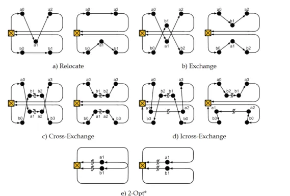
Local search is an improvement heuristic and as such it needs an initial solution as input. This set of methods perform a set of operations on a given solution aiming to improve it (Cari´c et al., 2008). Local search operators can be divided in two large sets - intra routes and inter routes.

Intra routes operators (Figure 3.7) perform operations on a single route at the time. These operators rearrange the sequence of the nodes in a route in order to make it more efficient. Some of the intra routes operators are:

(38)

3.6 Meta-heuristics • Relocate • Exchange • 2-Opt • Or-Opt

Figure 3.7: Intra route operators (Cari´c et al., 2008).

On the other hand, inter route operators (Figure 3.8) perform operations on two routes. These methods swap or rearrange the nodes between two routes in order to improve their quality and, consequently, to improve the solution. Some of the inter route operators are:

• Relocate • Exchange • Cross-Exchange • Icross-Exchange • 2-Opt*

Algorithm 4 describes generically the sequence of steps of the local search methods. As stated earlier, improvement heuristics can stop when it is not possible to improve the current solution. Like the constructive heuristics there is no guarantee that the pro-duced solution is the global optimum. Improvement heuristics do not possess mechanisms to escape local minimums and to explore new directions. Escaping mechanisms and tech-niques belong to a different set of heuristics, usually called meta-heuristics.

3.6 Meta-heuristics

Meta-heuristics are a set of procedures that combine heuristic and non-deterministic meth-ods in order to perform an efficient search in the search space. Heuristic methmeth-ods allow

(39)

3.6 Meta-heuristics

Figure 3.8: Inter route operators (Cari´c et al., 2008).

Algorithm 4: Local search. input : Feasible Solution output: Best solution found

1 while stopping criteria is not satisfied do

2 Apply intra routes operators on current solution 3 Apply inter routes operators on current solution 4 if new solution is better than current solution then 5 Replace current solution with new solution

6 end

7 8 end

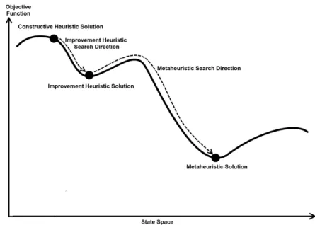
meta-heuristics to perform guided search to where a good solution might be. On the other hand, non-deterministic methods are used to escape local minimums and to explore new search directions. Usually meta-heuristics are used in combinatorial optimization prob-lems, in which routing problems are included.

Figure 3.9 represents the application of meta-heuristics to the solution produced by improvement heuristics in Figure 3.6. In this example the solution found by the meta-heuristic is indeed the global optimum but actually, in real cases there is no guarantee of its optimality.

It is important to mention that the input given to a meta-heuristic can be produced by any other methods, it does not have to be necessarily produced by improvement heuristics. Figure 3.9 is just an example of a possible sequence of steps to find an optimum solution.

(40)

3.6 Meta-heuristics

Figure 3.9: Solution produced by meta-heuristic.

3.6.1 Genetic Algorithms

Genetic algorithm is a meta-heuristic inspired on nature and on the way species evolve. According to the observations of Darwin, stronger species have greater probability to survive and to produce descendants at least as strong as their parents. In a similar way, weak species tend to produce weak descendants that tend to disappear over time. Genetic algorithms follow the idea described above and adapts it to solve numerous optimization problems.

Genetic methods systematically apply a set of operators (genetic operators) on a pop-ulation (set of possible solutions) in order to find an optimal or a near optimal solution (Ombuki et al., 2006).

Algorithm 5: Genetic algorithm.

input : G = (N , A) and set of UAVs V. output: Best solution found

1 Generate initial population

2 while stopping criteria is not satisfied do

3 Apply selection operators on initial population 4 Apply crossover on a newly formed population

5 Apply mutation operators on population from crossover 6 Replace initial population with a new one

7 end

Genetic algorithms are easy to implement and when all of the parameters are properly tuned it can produce good results. However, tuning genetic algorithms is a difficult and a time consuming task, it requires large set of tests in order to discover the best combination

(41)

3.6 Meta-heuristics

of parameters. Also it is important to notice that for different input the best combination of parameters may not be the same, meaning that it may be necessary to repeat the tun-ing process again. Another issue with genetic algorithms are the super individuals, i.e., solutions that are far better that the rest of the population. These solutions can quickly dominate the population and cause early convergence.

A more detailed description about different steps of genetic algorithms can be found in paper made by (Moura, 2008).

3.6.2 Tabu Search

Tabu search is an iterative meta-heuristic that performs an efficient space search by ex-ploring neighbours of the solution given as input (Tam and Ma, 2008). The tabu search accepts neighbours that are slightly worse than current solution. The admissibility of an inferior solution may seem as a bad strategy, however this method allows to escape local minimums and to explore new search directions.

To avoid exploration in an already explored directions, all solutions generated by tabu search are placed, for a certain number of iterations, in a tabu list. Tabu list is a mecha-nism that makes the search more efficient and guided. This way, each time a new solution is generated it is necessary to check if it is already on the tabu list. If a newly produced so-lution is better than the current one but, is already in the tabu list, then it will be dismissed. Tabu list can also be called as short term memory, since it only ”blocks” solutions for a short period of time. Besides the short term memory, tabu search has also an intermediate memory and a long term memory, which make the search even more efficient.

• Intermediate memory - contains rules of intensification that allow to perform guided search in a direction where an optimum solution might be. Intensification rules perform only small changes in current solution in order to avoid deviation from the current search direction.

• Long term memory - contain rules of diversification that allow the algorithm to explore new search directions. Diversification rules are a set of methods that can change the current solution in a drastic way and thus explore new search direc-tions. Normally, diversification rules are used when tabu search enters the stagna-tion phase.

Tabu search is a widely studied method and was largely applied in vehicle routing optimization problems. Results obtained by (Br¨aysy and Gendreau, 2002) show that tabu search is capable to find good solutions in short periods of time.

(42)

3.6 Meta-heuristics

Algorithm 6: Tabu search.

input : G = (N , A) and set of UAVs V. output: Best solution found

1 while stopping criteria is not satisfied do 2 Generate neighbourhood

3 Select best neighbour 4 Update current solution 5 Update tabu memory 6 end

3.6.3 Simulated Annealing

Simulated annealing is a set of procedures inspired on thermodynamic laws that describe atom’s behaviour at different temperature levels (Lin et al., 2011). When the temperature is high the atoms can move more easily, in routing optimization this state corresponds to a stage when it is possible to make drastic changes in the current solution. A lower temperature reduces the atoms movements (Figure 3.10). In optimizations problems this correspond to a neighbourhood exploration, i.e., only small changes are made in the cur-rent solution.

Figure 3.10: Entropy rate.

The main limitation of this method is the fact that it is difficult to discover when the temperature must be reduced. Despite that, results obtained by Chiang and Russell (1996) in VRP are very promising.

(43)

3.6 Meta-heuristics

Algorithm 7: Simulated annealing. input : G = (N , A) and set of UAVs V. output: Best solution found

1 while temperature != lower bound do

2 while number of tries for current temperature != 0 do 3 Randomize according to the current temperature 4 if new solution is better that current solution then 5 Replace current solution with new solution

6 end

7

8 end

9 Decrease temperature by specified rate 10 end

3.6.4 Multiple Ant Colony Systems (MACS)

This algorithm is based on the behaviour of ant colonies, where ants cooperate to achieve a certain goal. In multi ant colony systems (MACS), each colony tries to minimize a single objective of the original problem (Gambardella et al., 1999). For instance, in vehicle routing problems, one colony minimizes the number of mobile elements required and the other one minimizes the travelling time. However, optimizing each objective separately does not solve the original problem. This requires a cooperation between the ant colonies which is done by pheromones exchange that are left by each colony.

Figure 3.11: Multiple ant colony systems Gambardella et al. (1999).

Research by Gambardella et al. (1999) has a more detailed description about MACS and its methods.

(44)

3.6 Meta-heuristics

3.6.5 Guided Local Search

This method (Mills et al., 2003) is quite similar to the Local Search (Chapter 3.5.2). The main difference is that Guided Local Search can penalize the current solution in order to escape local optimums. When the algorithm enters into a stagnation phase, i.e., is trapped in local optimum, an augmented cost function is used. The idea behind the augmented cost function is to penalize neighbourhood solutions and consequently make all neigh-bourhood less attractive than other solutions located in more distant neighneigh-bourhoods and thus, deviate the search direction to other search spaces. The augmented cost function can be expressed in the following way:

h(s) = g(s) + λ × n X i=1 Pfi× Ifi (3.6) Where: • s current solution • g original cost function

• { f1, ..., fn } is a set of attributes that a solution possess

• Binary indication function Ifi, which determines if a certain attribute is present in a

solution.

• Penalization value Pfi, which penalizes solutions that have attribute fi. Initially set

to 0 but is adapted with time.

The parameter λ can be adapted to allow diversification or intensification of the search. Higher the value of λ more diverse will be the search, inversely lower the value of λ more directional and guided will be the search. Research performed by Kilby et al. (1997) show that this method is capable to find near optimum solutions in multiple cases of Solomon benchmark (Solomon, 1987).

(45)

C H A P T E R

4

Data Gathering in WSNs

4.1 Introduction

In previous sections the main challenges of the data gathering process have been stated. The mathematical formulation of the problem tackled in this thesis was introduced and some of general solving methods have been explored. In this section, the tackled problem will be reformulated, to incorporate the particularities of using mobile elements in WSNs, and a new hybrid heuristic approach to design paths for mobile elements in WSN will be presented and discussed.

4.2 Extended Problem

Given a set of sensor nodes that collect data about surrounding environment and a set o UAVs that will gather the data, the goal is to design an efficient set of paths to gather the data without violating the problem constraints.

Each sensor node has it own coordinates that identify its position. Moreover, each node has different buffer size to store the information and different sampling rate. This means that each node will fill its own buffer at different times. If the buffer size and the sampling are known then, it is possible to estimate the time window in which the buffer will be almost full and when it will be necessary to transfer the data to another entity, in this case the UAV. The transfer process changes according to the buffer size and throughput. By knowing these two informations it is possible to find out the time required to transfer the data from the sensor node to a UAV. To avoid losing the stored data, each node must be visited by an UAV within its own time window. Once the data is transferred to the UAV it must be delivered to the base station, for further processing, within a certain deadline. The deadline can be seen as a Time To Live (TTL), and in this case it is a time label. The data must be delivered to a base station within that TTL. However, if TTL is large the UAV can visit and gather the data from other nodes. The TTL restriction, which must be added to the initially discussed mathematical formalization of the data gathering problem (see Chapter 2.4), can be expressed mathematically as shown in expression 4.1.

(46)

4.2 Extended Problem X j∈N \{0}:ajv≥aiv X h∈N \{0} tjhxjhv ≤ DLi, ∀i ∈ C, ∀v ∈ V (4.1)

However, the constraint 4.1 can not be given as input to Mixed Integer Linear Pro-gramming (MILP) optimizers like CPLEX (IMB CPLEX, 2015) or Gurobi (Gurobi, 2015) as these solvers does not support the summation indexes that include variables. However, this limitation could be overcome by rewriting the constrain 4.1 as follows.

k_ivi = dli× X j∈N \{0} xijv, ∀i ∈ C, ∀v ∈ V (4.2) k_ivl − sj − tij + K(1 − xijv) ≥ kljv, ∀l ∈ C, ∀v ∈ V, ∀i ∈ C, ∀j ∈ N \ {0} (4.3) k_ivi ≥ 0, xijv ∈ {0, 1}, ∀i, j ∈ N, ∀v ∈ V (4.4) where: Sets V = {1, 2, ..., v} set of UAVs

N = {0, 1, ..., n, n + 1} set of nodes including the base station C = {1, 2, ..., n} set of nodes

Constants

dli delivery limit of node i

tij travel time between node i and j

si service time at node i

K is a large value

Decision variables

xijv one if UAV v ∈ V

travels from node i to node j, i, j ∈ N ki

jv remaining delivery limit time

if vehicle v ∈ V

is carrying data belonging to node i ∈ C The expanded constraints 4.2 and 4.3,originated from 4.1, ensure that the delivery limit value, of data collected at any node i ∈ C, decreases until the base station is reached. This decrease takes the travel and service time into consideration. Since all variables are non negative, data will not arrive outdated to the base station.

Overall, the problem to be solved is a Data Gathering Problem (DGP) applied to WSNs. In this case in particular, such DGP can be stated as a Vehicle Routing Problem with Time Windows (VRPTW), described in Chapter 2.4, with extra constraints so that:

(47)

4.2 Extended Problem

data collected from a specific node reaches the base station within a certain time, called delivery limit and denoted by dlni. That is, data has an expiration, or time-to-live (TTL),

label meaning that it can not arrive outdated at the base station. Vehicle routing and scheduling problems are known to be NP-hard, see (Lenstra and Kan, 1981), meaning that the DGP will also be hard to solve within an acceptable period of time.

4.2.1 Input and Output

Now that the problem has been clearly defined, it is possible to identify what will be the input and the output for the purposed algorithm. The input information must contain:

• A set of sensor nodes. Where each node has: – geographical coordinates

– buffer size

– time windows - start and end time – delivery limit (TTL)

• A set of UAVs characterized by its: – Travelling speed

– Buffer size

• A graph with information about the edges linking the sensor nodes • Throughput during data transfer

With these input parameters, the algorithm must minimize the distance and the number of paths required to gather the data from all sensor nodes. The output must provide detailed information about the obtained solution:

• Number of paths • Total distance

• Distance of each route • Duration of each path • Sequence of visited nodes • Arrival time to each sensor node • Departure time from each node

Route planning in wireless sensor networks for data gathering purposes

UNIVERSIDADE DO ALGARVE