Publishing House A K A P I T
C
OMPUTER
M
ETHODS IN
M
ATERIALS
S
CIENCE
Informatyka w Technologii Materiałów
Vol. 9, 2009, No. 2
AN IMPLICIT NUMERICAL INTEGRATION ALGORITHM FOR
BAI & WIERZBICKI (2007) ELASTO-PLASTIC MODEL
LUCIVAL MALCHER,FRANCISCO M.ANDRADE PIRES,
JOSÉ M.A.CÉSAR DE SÁ,FILIPE X.C.ANDRADE
Department of Mechanical Engineering, Faculty of Engineering, University of Porto Rua Dr. Roberto Frias, Porto 4200-465, Portugal
Corresponding Author: [email protected]; (L. Malcher)
Abstract
This contribution describes an implicit algorithm for numerical integration of a recently proposed model for metal plasticity and fracture [2]. The constitutive equations of the material model critically include both the effect of pressure through the triaxiality ratio and the effect of third deviatoric stress invariant through the lode angle in the description of material. These effects are directly introduced on the hardening rule of the material. The theoretical basis of the material model is presented in the first part of the paper. Then, the necessary steps required to implement the model within an im-plicit quasi-static finite element environment are discussed. In particular, the stress update procedure, which is based on the so-called operator split concept resulting in the standard elastic predictor/return mapping algorithm, and the computa-tion of tangent matrix consistent with the stress update are described. Finally, the simulacomputa-tion of a flat grooved specimen subjected to tension [1] is presented to illustrate the robustness and efficiency of the proposed algorithm.
Key words: finite element method, elasto-plastic model, hydrostatic pressure sensitivity, lode angle dependence
1. INTRODUCTION
One of the most commonly used models to de-scribe the behavior of metals is the von Mises model. According to this model, plastic yielding begins when the second invariant of the deviatoric stress tensor, , reaches a critical value. The pres-sure component of the stress tensor does not take part in the definition of yielding and consequently the model can be regarded as “pressure-insensitive” [5]. Another feature of the model, when compared to other material models, is that it is also independent of the third invariant of the deviatoric stress tensor. Both parameters have got a well known influence on the yield surface [8]. The level of hydrostatic is re-sponsible for controlling the size of the yield surface and the third invariant is responsible for the shape of the yield surface [1].
The importance of the hydrostatic stress and lode angle has been recognized by several authors and introduced into the constitutive description of some materials such as soils, rocks and concrete [2,8]. In the case of ductile materials, which are addressed in this paper, many researchers have conducted exten-sive experimental studies. Richmond and Spitzing [6] were among of the first researchers to investigate the effect of pressure on yielding of aluminum alloys.
Ductile fracture is a local phenomenon and the state of stress and strain, at the expected fracture location, must be determined with accuracy. Frac-ture initiation is often preceded by large plastic de-formation and there are considerable stress and strain gradients around the point of fracture. In this case, the theory is not accurate enough and more refined plasticity models have to be introduced.
C OMPUTER M ETHODS IN M ATERIALS S CIENCE
The determination of an adequate shape of the yield surface has become an important issue in sheet metal forming. In this case, the von Mises plane stress ellipse does not lead to a correct prediction of necking instability. To overcome some of the previ-ous limitations, Bai & Wierzbicki [2] have proposed a model that includes both the effect of pressure and the third invariant on the evolution of plastic flow.
Preliminaries
For the sake of completeness and notation clar-ity, we will briefly summarize some fundamental relations commonly used in plasticity. The stress tensor can be split in two components: an hydro-static and a deviatoric component, which can be represented as:
(1) The strain tensor can also be split in two
compo-nents:
(2)
where, is the stress tensor, 2 is
the deviatoric stress tensor,
represents the pressure or hydrostatic stress, is the elastic strain tensor, is the deviatoric strain tensor and represents the volumetric strain. The con-stants and are, respectively, the shear modulus and the bulk modulus. We can also define the equivalent stress, which is a function of the second invariant of deviatoric stress tensor, as:
3 (3)
where, is the equivalent stress, is the second invariant of the deviatoric stress and represents the norm of the deviatoric stress tensor.
The third invariant is a scalar quantity that is ob-tained by computing the determinant of the devia-toric stress tensor, denoted by . Alterna-tively, the third invariant can be expressed by:
(4) The influence of pressure on the von Mises elasto-plastic model can be introduced through the triaxiality ratio which is a dimensionless hydrostatic stress. The triaxiality ratio is defined as the ratio between the pressure and the equivalent stress:
(5)
The third invariant of the deviatoric stress tensor can be normalized and related with the so-called lode angle through the expression:
. cos 3 (6)
where, is the normalized third invariant and is the lode angle. Since the range of the lode angle is 0 ⁄ , the range of has to be 13
1. The lode angle can also be normalized by:
1 1 (7)
where, is the normalized lode angle. The range of is 1 1. The parameter will be called the lode angle parameter hereinafter.
2. THE BAI & WIERZBICKI YIELD FUNCTION
Bai & Wierzbicki [2] have proposed an elasto-plastic model that includes both the effect of pres-sure (through the triaxiality ratio) and the effect of the third invariant of the deviatoric stress tensor (through the lode angle). These effects are intro-duced by redefining the hardening rule. While in the classic von Mises model, the hardening rule is only a function of the accumulated plastic strain, , in Bai & Wierzbicki´s model the hardening rule is a function of the accumulated plastic strain, the tri-axiality ratio and the parameter , which is a function of the load angle. The hardening rule is rewritten as:
, , . 1 .
(8) where, is the material strain hardening func-tion, , , , and are experimental parame-ters, is the reference value of the triaxiality ratio and is a parameter defined as a function of the lode angle: cos ⁄6 1 cos ⁄6 1 cos ⁄6 1 ⁄ ⁄ . sec ⁄6 1 (9)
The effect of the triaxiality ratio and load angle are included on the hardening rule through the
pa-rameters 1 and
, respectively. The new yield criterion is simply obtained by replacing
C OMPUTER M ETHODS IN M ATERIALS S CIENCE
the standard hardening rule by , ,
on the von Mises yield function, which can be repre-sented by Φ, as:
Φ . 1 .
(10) In order to understand the above yield function, let us analyze the influence of some experimental pa-rameters , , , , on the behavior of the model. The parameter is a material constant that needs to be experimentally calibrated and that de-scribes the effect of the hydrostatic pressure on the material plastic flow. If 0, the model loses the dependence of the triaxiality (and of the hydrostatic pressure) and recovers, as a limiting case, the behav-ior of the von Mises model.
The reference triaxiality, , depends on both the type of load applied and the geometry of the speci-men. For a smooth bar subjected to tension, takes the value equal to 1 3⁄ , for a cylindrical specimen under compression is equal to 1 3⁄ and for both torsion and shear tests is equal to 0. With regard to the third invariant effect, the experimental parameter can assume one of two forms, ac-cording to the value of the normalized lode angle .
0
0 (11)
The parameter also depends on the type of test. For example, if a smooth bar is used in a tensile test 1, if a torsion test 1, if a cylinder specimen is used in a compressive test 1. The convexity of the yield surface is controlled by the ratio of these parameters. The range of the parameter
is between 0 1. When 0 it
corre-sponds to plane strain or shear condition, when 1 it corresponds to axisymmetric problem. The introduction of the term is done to ensure the smoothness of yield surface and its differentiability with respect to lode angle around 1.
3. NUMERICAL INTEGRATION ALGORITHM
An algorithm treatment of the model summa-rized in section 2 relies on the operator split meth-odology, which results in an elastic predictor/plastic corrector algorithm [4,7]. In the elastic predictor phase (obtained by freezing the plastic flow during
the time interval [ , ]), values from the previ-ous converged solution are used as initial conditions to evaluate the elastic trial state, i.e., the exact elastic solution.
If the yield condition is violated, the plastic cor-rector is initiated based on the Newton-Raphson procedure. The governing equations for one step of the Newton-Raphson iterative scheme are summa-rized in Box 1.
4. NUMERICAL EXAMPLE
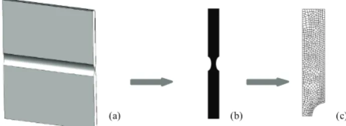
This section presents an example to illustrate ba-sic aspects of the proposed integration algorithm described previously. A tensile test of flat grooved plates, as shown in figure 1, is used to illustrate the numerical performance of the proposed algorithm within an implicit quasi-static finite element envi-ronment. The relative residual of the solution is pre-sented to show the asymptotic convergence of the algorithm.
The specimen has been subjected to monotonic axial stretching and the numerical results are com-pared with experimental results reported by Bai et al [2]. The material properties including the pressure effect and lode dependence constants, adopted in the present analysis, are listed in table 1. These parame-ters were taken from Bai [1] for an aluminum alloy.
Fig. 1. (a) Flat grooved specimen, thickness = 2.11 mm, groove
radius = 1.59 mm, width = 50 mm, plate thickness = 5 mm. (b) a longitudinal section of the specimen and (c) Finite element mesh: 1981 nodes and 616 elements.
Table 1. Calibrated material properties of aluminum 2024-T351.
Basic material properties lode constants Pressure and
Description Symbol Value η0 1/3
Density ρ 2.7 103 Kg/m3 C η 0.009 Elastic Modulus E 7.115 105 [MPa] Cθt 1.0 Poisson´s ratio ν 0.3 Cθs 0.855 Initial yield
stress σy0 370 [MPa] Cθc 0.90
Hardening
curve σy( )
908(0.0058+ )0.1742
[MPa] m 6
C OMPUTER M ETHODS IN M ATERIALS S CIENCE
where , and are the residual functions for each variable of the problem. represents the flow vector and can be defined as:
. The parameters , and are
obtained through the equations: 1
. . . . , . . . and
. . .. .
In order to highlight the convergence of the Newton-Raphson algorithm in table 2, we present the relative residual of the solution for two typical load increments when we have both pressure effect and lode angle dependence introduced. The conver-gence rates, in both of case, are clearly quadratic.
In the figure 2, we can analyze the behavior of the reaction-displacement curve (a) and the accumu-lated plastic strain-displacement curve (b) obtained numerically. Verifying first the curve reaction-displacement, figure 2(a), the result obtained without
Table 2. Convergence table for two typical load increments.
Flat grooved specimen.
including any effect 0, 1, 1,
1, 0 , reproduces the von Mises model. In this case, the error is around 17%, between experimental and numerical results. If only the pressure effect is
included 0.09, 1, 1, 1,
0 , the results are similar with Drucker Prager model and the error between the numerical simulation and the experimental one are smaller than the previous case, but still big. In this case, the error is about 13%. Finally, we can introduce both the pressure Box 1: Fully implicit Elastic predictor/Return mapping algorithm.
Iteration
number Relative residual [%] Iteration number Relative residual [%]
1 0.51275x10⁻² 1 0.17977x10⁻¹
2 0.37416x10⁻⁴ 2 0.44738x10⁻³
3 0.21888x10⁻⁸ 3 0.27548x10⁻⁶
4 0.12611x10⁻¹⁴ 4 0.10461x10⁻¹²
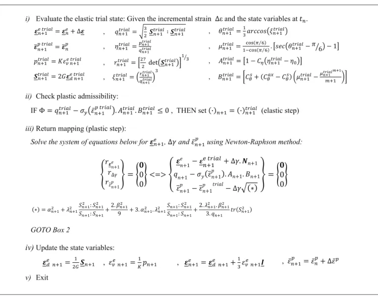
i) Evaluate the elastic trial state: Given the incremental strain and the state variables at .
, ,
, ,
, ,
, ,
ii) Check plastic admissibility:
IF , THEN set (elastic step)
iii) Return mapping (plastic step):
Solve the system of equations below for , and using Newton-Raphson method:
GOTO Box 2
iv) Update the state variables:
, , ,
C OMPUTER M ETHODS IN M ATERIALS S CIENCE
where, and represent the updated yield function and the updated von Mises equivalent stress, respec-tively, on the discretizated step . The variable
represents the accumulated plastic strain at . The variable ∆ represents the plastic
multiplier and represents the yield stress for the conventional von Mises model.
effect and lode angle dependence 0,
0.855, 1, 0.90, 6 . In this case, the
reaction-displacement curve agrees well with the experimental results. The error is less than 2%.
By analyzing the accumulated plastic strain-displacement curve, figure 2(b), we can observe the evolution of the accumulated plastic strain as a func-tion of the prescribed displacement. We can verify
that only with pressure effect and with both pressure effect and lode angle, the growth rate of the accumu-lated plastic strain is faster than without effects intro-duced. In addition, we can conclude that the Bai & Wierzbicki elasto-plastic model reaches higher levels of plastic strain, even for lower levels of equivalent stress, when we have both effects included.
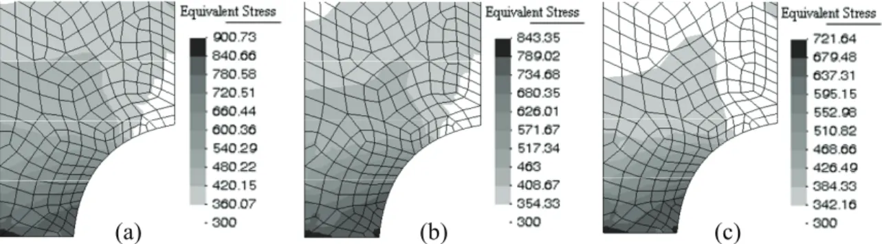
From figure 3, we can determine the point of maximum and minimum equivalent stress for all numerical simulations. For the von Mises model, the maximum equivalent stress attains a value of 900.73 MPa. If only the pressure effect is included, the maximum equivalent stress is equal to 843.35 MPa. When both effects are included, the maximum equivalent stress is equal 721.64 MPa. The maxi-mum value is always located on the central point of Box 2: The Newton-Raphson algorithm for solution of the return mapping system of equations.
1) Initialize iteration counter, , set initial guess for , and
corresponding residual:
2) Perform Newton-Raphson iteration
New guess for , and :
, and
Update stress tensor:
, and
together with other elasto-plastic parameters: , , , , and
3) Check for convergence
IF THEN RETURN to Box 1.
C OMPUTER M ETHODS IN M ATERIALS S CIENCE
the specimen. The experimental results agree with the numerical simulations when we have the pres-sure effect and lode dependence introduced.
5. CONCLUSION
In this paper was presented an implicit numerical integration for a recently proposed elasto-plastic model that includes the pressure effect and lode an-gle dependence into the hardening rule. The conver-gence of the Newton Raphson algorithm is similar between von Mises model and Bai & Wierzbicki model without effects introduced and between Drucker Prager and Bai & Wierzbicki model with only pressure effect introduced. The numerical
simu-lation of a flat grooved specimen of the aluminum alloy was used to illustrate the robustness of the proposed algorithm, we verified that both effects
have to be taken into account on the plastic flow. The error in the reaction-displacement curve for a total displacement of 0.2 [mm] was reduced from 17% to 2% by including both the effect of pressure and lode angle.
REFERENCES
1. Bai, Y., Effect of Loading History on Necking and Frac-ture, Ph.D Thesis, Massachusetts Institute of Technology, 2008.
2. Bai, Y., Wierzbicki, T., A new model of metal plasticity and fracture with pressure and lode dependence, Int. J. of Plasticity, 2007, doi:10.1016/j.ijplas.2007.09.004.
a) b)
Fig. 2. Reaction-displacement curve (a) and accumulated plastic strain-displacement curve (b) for Bai and Wierzbicki model: without
effects (or von Mises model), with only pressure effect included (or Drucker Prager model) and both pressure effect and lode angle dependence included.
Fig. 3. Equivalent stress parameter plotted through the mesh. (a) without effects or von Mises model, (b) only with pressure effect or
Drucker Prager model, and (c) both pressure effect and lode angle dependence.
C OMPUTER M ETHODS IN M ATERIALS S CIENCE
3. Bao, Y., Predition of Ductile Crack Formation in Un-crecked Bodies, Ph.D Thesis, Massachusetts Institute of Technology, 2003.
4. De Souza Neto, E. A., Peric, D., & Owen, D. R., Computa-tional Methods for Plasticity: Theory and Application. Wiley, 2008.
5. Hill, R., The Mathematical Theory of Plasticity, Oxford Univ. Press, London, 1950.
6. Richmond, O., Spitzig, W.A., Pressure dependence and dilatancy of plastic flow. In Theoretical and Applied Me-chanics, Proc. 15th Int. Congress of Theoretical and Ap-plied Mechanics., Toronto, North-Holland Publ Co, Am-sterdam, 1980, 377–386.
7. Simo, J., Hughes, T., Computational Inelasticity, Springer, 1998.
8. Wilson, C.D., A critical reexamination of classical metal plasticity, Journal of Applied Mechanics, Transactions ASME, 69(1), 2002, 63–68.
NIEJAWNY ALGORYTM CAŁKOWANIA NUMERYCZNEGO DLA SPRĘŻYSTO-PLASTYCZNEGO MODELU BAI – WIERZBICKIEGO
Streszczenie
Niniejszy artykuł opisuje niejawny algorytm całkowania numerycznego modelu plastyczności i pękania metali. Równania konstytutywne modelu materiału uwzględniają zarówno wpływ ciśnienia przez wprowadzenie współczynnika trójosiowowości i wpływ trzeciego niezmiennika dewiatora tensora naprężenia. Te efekty bezpośrednio wpływają na sposób umacniania się materiału. W pierwszej części artykułu przedstawiono podstawy teoretyczne modelu materiału. Następnie omówione są kroki niezbędne do implementacji modelu w niejawnym quasi-statycznym środowisku elementów skończonych. W szczegól-ności opisane zostały: procedura uaktualniania naprężenia, która opiera się na tak zwanym podziale operatora oferującym stan-dardowy algorytm odwzorowania w stanie sprężystym oraz na procedurze obliczania macierzy stycznych spójnej z uaktualnia-niem wartości naprężeń. W końcowej części pracy przedstawio-no symulację rozciągania płaskiej próbki z rowkami w celu pokazania wiarygodności i skuteczności proponowanego algo-rytmu.
Received: October 8, 2007 Received in a revised form: November 6, 2007 Accepted: November 6, 2007