Crop data retrieval using earth observation data to support agricultural water management

ISSN: 1809-4430 (on-line) www.engenhariaagricola.org.br

2 _{Instituto Dom Luiz (IDL), Faculdade de Ciências, Universidade de Lisboa, 1749-016 Lisboa/ Lisboa, Portugal.} 3 _{Faculdade de Ciências, Universidade de Lisboa, 1749-016 Lisboa/ Lisboa, Portugal.}

Received in: 5-7-2018 Accepted in: 3-21-2019

Doi: http://dx.doi.org/10.1590/1809-4430-Eng.Agric.v39n3p380-390/2019

TECHNICAL PAPER

CROP DATA RETRIEVAL USING EARTH OBSERVATION DATA TO SUPPORT

AGRICULTURAL WATER MANAGEMENT

João Rolim

_{, Ana Navarro}

_{, Pedro Vilar}

_{, Cátia Saraiva}

_{, Joao Catalao}

1*_{Corresponding author. LEAF - Linking Landscape, Environment, Agriculture and Food, Instituto Superior de Agronomia,}

Universidade de Lisboa, 1349-017 Lisboa/ Lisboa, Portugal.

E-mail: joaorolim@isa.ulisboa.pt | ORCID ID: https://orcid.org/0000-0003-1782-2732

KEYWORDS

remote sensing,

irrigation, software,

NDVI, crop

phenology, crop

coefficient.

ABSTRACT

Accurate crop data are essential for reliable irrigation water requirements (IWR)

calculations, which can be acquired during the crop growth season for a given region

using earth observation (EO) satellite time series. In addition, a relationship between crop

coefficients and the NDVI can be established to allow for crop evapotranspiration

estimation. The main objective of the present work was to develop a methodology, and its

implementation in an application software, to extract crop parameters from EO image

time series for a set of parcels of different types of crops, to be used as input data for a soil

water balance model to compute IWR. The methodology was tested at two distinct test

sites, the Vila Franca de Xira (site I) and Vila Velha de Ródão (site II) municipalities,

Portugal. Landsat-7 and -8 images acquired from April to October 2013 were used for site

I, while SPOT-5 Take-5 images from April to September 2015 were considered for site II.

EO data were used to estimate the basal crop coefficients, planting dates, and crops

growth stage lengths. Based on crop, soil and meteorological data, the IWR for the main

crops of both test regions were estimated using the IrrigRotation model. The crop

coefficient curves obtained from the EO data proved to be reliable for IWR estimation.

INTRODUCTION

Reliable IWR estimation requires available and accurate data (e.g., crop coefficients, planting dates, and crop growth stage lengths) to determine the soil water balance. Crop data can be estimated using acquired earth observation (EO) data, along the crop growth cycle, at time intervals suitable for the detection of changes in crop phenology (D’Urso & Calera Belmonte, 2006; Vilar, 2015; Vilar et al., 2015; Navarro et al., 2016; Rolim et al., 2016). Presently, the availability of free and open access to high spatial resolution EO data with a short revisit time allows for accurate crop parameter estimation as well as crop growth cycle characterization, improving the identification of each growth cycle stage, which is often imperceptible when lower temporal resolution data are used (El Hajj et al., 2009; D’Urso et al., 2010; Ramme et al., 2010; Johann et al., 2013; Johann et al., 2016; Navarro et al., 2016; Rolim et al., 2016; Grzegozewski et al., 2017; Toureiro et al., 2017).

EO methodologies have been widely used for crop evapotranspiration (ETc) and IWR estimation because of

the reflective properties of vegetation that allow one to estimate crop biophysical parameters and plant processes such as transpiration (Neale et al., 1989; Calera Belmonte et al., 2005; D’Urso et al., 2010; Paço et al., 2014; Vuolo et al., 2015; Ferreira et al., 2016; Oliveira et al., 2016). ETc

can be estimated from EO data using empirical methods based on the use of vegetation indices (VIs) to estimate crop coefficients (Neale et al., 1989; Calera Belmonte et al., 2005; D’Urso et al., 2010) or using physics-based methods based on the surface energy balanceto estimate the latent heat flow based on EO thermal images (Bastiaanssen et al., 1998; Allen et al., 2007; Eldeiry et al., 2016). The empirical methods have been more widely used because of their simplicity, with the most common VI, the normalized difference vegetation index (NDVI), used to estimate several crop parameters, such as fraction of ground cover (fc), single crop coefficient (Kc), and basal

crop coefficient (Kcb), among others, used as input data for

soil water balance simulations (D’Urso et al., 2010). IWR estimation is commonly performed using the crop coefficient approach(Allen et al., 1998), computing ETc based on the use of crop coefficients that relate the ETc

to the reference evapotranspiration (ETo). ETo is calculated

by using the standard FAO Penman–Monteith method (Allen et al., 1998). The crop coefficients can be estimated using the single crop coefficient (Kc) or the dual crop

coefficient approach, based on Kcb and on the soil

evaporation coefficient (Ke) (Allen et al., 1998). As

proposed by several authors (Neale et al., 1989; Calera Belmonte et al., 2005; D’Urso & Calera Belmonte, 2006; D’Urso et al., 2010), the Kcb-NDVI approach establishes

an empirical relationship between the Kcb values, obtained

through field measurements (soil water balance, lysimeters, micrometeorological techniques, etc.), and NDVI values retrieved from optical EO time series. The equations used to estimate crop coefficient values based on VIs require field campaigns to be calibrated and validated for a given location. Once calibrated, they can accurately estimate ETc, enabling one to replace in situ data, which

are difficult and expensive to collect at field evaluations (D’Urso et al., 2010; Toureiro et al., 2017).

In both crop coefficient approaches the main source of uncertainty in the IWR estimation is the incorrect characterization of the crop growth stage lengths and hence of the crop coefficient curves (Allen et al., 1998; Toureiro et al., 2017). In fact, IWR estimation for water management purposes is often performed using FAO 56 tabulated crop coefficients values and lengths of crop growth stages that can lead to large errors (Allen et al., 1998). The uncertainty resulting from the use of these values is increasingly relevant because of climate change, with impacts on crop calendars and phenology, requiring field observations for new crop data collection. Therefore, EO techniques are a viable and cost-effective alternative to complement traditional field evaluations.

The main objective of this work was the development of a methodology to extract crop data from EO time series, for several crop parcels of an irrigation perimeter, to be used as input data for a soil water balance model, enabling crop IWR calculation at a regional level. More specifically, it was intended to use EO data to estimate basal crop coefficients, planting dates, and crop growth stage lengths. The developed methodology was

implemented in an application software (Vilar, 2015) and applied to two different test sites in Portugal, the Vila Franca de Xira (site I) and Vila Velha de Ródão (site II) municipalities, where EO images of different spatial and temporal resolutions were used.

METHODOLOGY NDVI TIME SERIES

NDVI values were calculated for each EO data acquisition date using the red and near infrared bands using [eq. (1)] (Rouse et al., 1974) as follows:

R NIR R NIR

NDVI















in which ρNIR and ρR are the surface reflectance in the near

infrared and red bands, respectively. Based on the NDVI time series, for each crop parcel, characterization of the behaviour of each crop type throughout the entire growing season and extraction of crop data were possible.

BASAL CROP COEFFICIENT CURVE

Kcb values are empirically determined from the Kcb

-NDVI relationships applied within the PLEIADeS project using [eq. (2)] (Calera Belmonte et al., 2005; D’Urso & Calera Belmonte, 2006) as follows:

1

0

5625

1

.

NDVI

.

K







in which NDVI is the mean value of each parcel for each acquisition date. This equation was defined using several types of annual crops, including maize, in a pilot campaign in the Barrax municipality in Spain, with a Mediterranean climate, and showed good agreement between field measurements and estimated Kcb-NDVI values (Calera

Belmonte et al., 2005; D’Urso, & Calera Belmonte, 2006). NDVI time series were used to define the crop coefficient curve, enabling one to identify the crop growth stage lengths (initial, crop development, mid-season and late season) and the corresponding Kcb coefficients for

the initial (Kcb ini), mid-season (Kcb mid), and end of late

season (Kcb end) stages (Figure 1), reflecting the actual crop

growth conditions.

IRRIGATION WATER REQUIREMENTS (IWR) IWR are defined as the net amount of water, expressed as the depth of water (mm), applied to the crop throughout the entire irrigation season to fully satisfy the water loss via evapotranspiration that is not satisfied by rainfall or soil water storage and not considering irrigation losses (Doorenbos & Pruitt, 1977; Allen et al., 1998). In this study, IWR were computed using the IrrigRotation soil water balance simulation model (Rolim & Teixeira, 2008). This model simulates the soil water balance using a daily time step and computes ETc according to the dual crop

coefficient approach proposed by Allen et al. (1998), as defined in [eq. (3)] as follows:





c

K

K

K

ET

ET









in which ETc is the crop evapotranspiration (mm·day−1),

Kcb is the basal crop coefficient, Ke is the soil evaporation

coefficient, Ks is the water stress coefficient and ETo is the

reference evapotranspiration (mm·day−1_{). K}

s describes the

effect of water stress on crop transpiration, yet, in this case, no water stress was considered when simulating the soil water balance. Alternatively, Kcb values retrieved from

EO data are already adjusted to the actual field conditions, which already incorporate water stress. ETo was computed

using the FAO Penman–Monteith (FAO-PM) method (Allen et al., 1998).

The soil water balance equation adopted in the IrrigRotation model is defined as follows:



P

ET

R

E

A

D



R















in which ΔR is the variation in the volume of water stored in the root zone (mm), Δt is the time step (day), P is the precipitation (mm·day−1_{), Rg is the irrigation (mm·day}−1_),

Ac is the capillary rise (mm·day−1), ETc is the crop

evapotranspiration (mm·day−1_{), E}

s is the runoff

(mm·day−1_{) and D}

r is the drainage and deep percolation

(mm·day−1_{). In the present study, an irrigation strategy of}

no water restrictions was evaluated because the water deficit is included in the Kcb obtained using the EO data.

CROP DATA RETRIEVAL FROM EO DATA

A realistic estimate of the IWR depends on the choice of representative crop parcels. The analysis of just one or a few parcels for each type of crop might not allow for the identification of the standard pattern for each crop along its growth cycle, for one given region, because of noise and clouds in the satellite images and the lack of representativity. Thus, it is more useful to consider a broad set of crop parcels, with similar phenological behaviour, to extract average crop data values, as performed by Esquerdo et al. (2011) and Johann et al. (2013, 2016), which are more representative and reliable than those individually obtained, reducing uncertainty resulting from sensor errors and cloud cover and improving data reliability when IWR is calculated at a regional or irrigation perimeter level. Hence, two different approaches were adopted to retrieve crop data as follows:

Average curve: The average NDVI and Kcb values

were obtained for each parcel and for each acquisition epoch. Based on these values, the crop growth cycle curves were defined by calculating the average NDVI and

Kcb values of all the crop parcels of the same type, also

determining the maximum and minimum values, to present the dispersion of the values acquired by the satellite. This approach aimed to extract the Kcb time series and the

identification of the crop growth stages dates using an average value for each crop to be used as an input for the soil water balance model.

A set of curves: The NDVI, and Kcb time series

were determined for each individual parcel, as previously mentioned. The crop growth cycle curve of all parcels, of the same type of crop, were simultaneously plotted in one single chart, showing the dispersion of the results. This second approach allowed one to identify different crop growth behaviours, and consequently to detect different crop varieties or the presence of outlier parcels. Removing these parcels, or separating them into subsets, improved the representativeness of each type of crop data. Comparing the NDVI (or Kcb) curves obtained for several

parcels enabled us to distinguish different crop developmental patterns, reflecting distinct crop growth and management conditions such as different crop varieties, planting date, plant density, irrigation, fertilization and pest and diseases control levels, allowing for the detection of different productivity levels. Esquerdo et al. (2011) generated NDVI time series for several soybean parcels in Brazil, aggregated at the municipality level, demonstrating the usefulness of adopting several parcels to generate an average NDVI profile allowing for an accurate characterization of this crop’s phenological cycle.

COMPUTATIONAL APPLICATION DEVELOPED APPLICATION STRUCTURE

A computational application was developed using MATLAB® 2014 to implement the proposed methodology (Vilar, 2015). This application was composed of three

computational modules, including a Geographic

Information System (GIS) graphical user interface and a geospatial database in ArcCatalog®. The database stores information regarding the crop parcels and crop biophysical parameters provided by the EO data. This application was developed to automate EO time series processing for a large number of crop parcels.

APPLICATION SOFTWARE WORKFLOW

The application comprises three modules (Figure 2) as follows:

- Module I – Optical digital image processing for data extraction: This module aims to extract information from EO optical images time series. NDVI values are calculated based on [eq. (1)]. Results, for each input file, are the NDVI images. Land Surface Temperature (LST) values are also calculated by this software for each crop parcel, despite not being used in this study.

- Module II – Kcb calculation using the GIS

interface: This module performs the average Kcb

calculation for each crop parcel based on the NDVI images using the ArcMap® Zonal Statistics tool. The Kcb

estimation is performed based on the NDVI time series images using [eq. (2)]. Kcb values are then used to generate

- Module III – Crop growth stages estimation: This module plots the NDVI and Kcb time series curves

graphs for each crop type based on the attribute table previously generated by module II and on the approach selected (average curve or a set of curves), allowing one to observe crop behaviour along the entire growing season. INPUT DATA

The main input data used for this application software are composed of the following:

- Optical image time series acquired by the Landsat-7 Enhanced Thematic Mapper plus (ETM+)

sensor and the Landsat-8 Operational Land Imager (OLI) from April to October 2013 for test site I.

- Optical image time series acquired by the SPOT-5 Take-5 HRG (High Resolution Geometric) sensors, from April to September 2015, for test site II.

- Vector files extracted from the National Land Parcel Identification System (NLPIS) containing each agricultural parcel’s limits, as well as the crop type, for the 2013 (site I) and 2015 (site II) subsidy control campaigns. These files were provided by the Portuguese Control and Paying Agency (Instituto de Financiamento da Agricultura e Pescas – IFAP).

FIGURE 2. Flowchart of the application software. OUTPUT DATA

- NDVI images generated, using module I, to be used as input to the Kcb calculation procedure (module II).

The NDVI and LST images can also be used for other type of applications beyond the scope of IWR estimation, such as crop parcel classification (Vilar et al., 2015).

- NDVI and Kcb time series graphs that allow one to

characterize the crop behaviour along the growth cycle and, consequently, distinguish the four different crop growth stages and the corresponding Kcb ini, Kcb mid and Kcb end values, enabling the definition of the crop coefficient

curve as shown in Figure 1.

EXPERIMENTAL APPLICATION

The developed methodology was applied to evaluate its suitability to retrieve crop parameters from EO data to be used as input data for a soil water balance model to estimate IWR. This study was conducted at two test sites in central Portugal (Figure 3). For both sites, the location of the agricultural parcels belonging to the crop types of interest was selected based on the NLPIS data. For each acquisition date, and for every parcel, the average NDVI values were determined to estimate the Kcb values,

planting dates and crop growth stage lengths. Based on crop, soil and meteorological data, the IWR were estimated using the IrrigRotation model for the main crops at both sites.

TEST SITE I – VILA FRANCA DE XIRA

The first test site is in the Vila Franca de Xira municipality, in the Lisbon District, Portugal, as shown in Figure 3. The main annual irrigated crops produced in this region are maize, tomato, rice and melon (Vilar et al., 2015). The Vila Franca de Xira climate, according to the Köppen classification system, is Csa, i.e., a temperate climate with a hot and dry summer. Climate normal data, from 1971 to 2000, for the Lisboa weather station (38º 43’

N, 9º 08’ W, 77 m in altitude) of the Instituto Português do Mar e da Atmosfera (IPMA) network, show that the hottest month is August, with a monthly average temperature of 23ºC, and the lowest average temperature of 11.3ºC is observed in January. The highest monthly precipitation occurs in December (121.8 mm), while July is the driest month (6.1 mm). The average annual precipitation during the period of record is 725.8 mm.

FIGURE 3. Location of the test sites: Vila Franca de Xira (test site I) and Vila Velha de Ródão (test site II) municipalities. DATA

Earth Observation (EO) data

Two Landsat-7 satellite ETM+ and 9 Landsat-8 OLI/TIRS sensor images acquired from April to October 2013 were used (Vilar, 2015; Vilar et al., 2015),

corresponding to the spring/summer crop growing season (Table 1). The spatial resolution of both images is 30 m with a revisit time of 16 days. The acquisition dates, and the corresponding day of the year (DOY) and type of image, are listed in Table 1.

TABLE 1. Landsat-7 (L7) and Landsat-8 (L8) images acquisition dates for site I (DOY - Day of the Year, 2013 in this case).

Satellite L8 L7 L8

Date 17/04 11/05 12/06 20/06 6/07 22/07 7/08 23/08 8/09 24/09 10/10

DOY 107 131 163 171 187 203 219 235 251 267 283

Radiometric calibration and normalization of the Landsat images

Landsat-7 and Landsat-8 data were downloaded as Level-1 data products consisting of quantized and calibrated scaled Digital Numbers (DN) representing the multispectral image data. All images were rescaled to top of atmosphere (TOA) reflectance using radiometric rescaling coefficients provided in the metadata file (MTL.txt) that is delivered with the Level-1 product. The conversion to TOA reflectance was performed using equations provided at the United States Geological Survey (USGS) website. Landsat-7 images were used in this study to fill missing data in the time series, as most of the crop parcels were covered by clouds in the Landsat-8 images

acquired during May (DOY 139) and in the first half of June (DOY 155), 2013. Despite the Landsat-7 Scan Line Corrector (SLC) malfunction, it was possible to use these images because Vila Franca de Xira (site I) is in the central part of the images not affected by the sensor error.

To compare data from different sensors (with slightly different wavelength intervals), a relative radiometric normalization was applied to both Landsat datasets (Du et al., 2002). The images normalization of the same region acquired at two different times (or by different sensors) is completed using a linear regression, assuming that the spectral reflectance properties of the sampled pixels did not change during the time interval. Based on two sets of pseudo-invariant features, bright (bare soil) and

dark (water), selected on both Landsat images (L7-DOY 131/L8-DOY 139 and L7-DOY 163 and L8-DOY 155) via visual inspection, it was possible to calculate the linear regression coefficients.

Soil Data

Sheets 390, 391 and 404 of the soil maps of Portugal, produced by the Instituto de Hidráulica, Engenharia Rural e Ambiente (IHERA), at a scale 1:25 000, were used for test site I to identify the soil types present in each crop parcel and consequently obtain the soil hydraulic characteristics to perform the soil water balance simulation.

Meteorological data

Climatic data was obtained from the Magos Dam weather station (38º 59’ N, 8º 42’ W, 43 m in altitude) belonging to the Sistema Nacional de Informação de Recursos Hídricos (SNIRH) for the period from April to October 2013 at a daily time step. The meteorological variables considered were the following: maximum air temperature (°C), minimum air temperature (°C), maximum relative humidity (%), minimum relative humidity (%), average wind speed at 2-m height (m∙s-1_),

solar radiation (MJ∙m-2_∙day-1_{) and precipitation (mm∙day}-1_).

RESULTS AND DISCUSSION NDVI time series

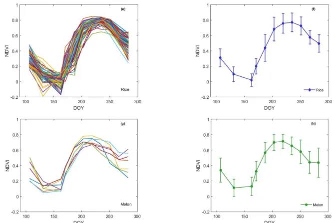
The time series of the mean NDVI for the selected crops (maize, tomato, rice, and melon) at test site I (Vilar et al., 2015) are shown in Figure 4, for the set of curves and average curve approaches, presenting the evolution of the crops’ NDVI temporal profiles as described in Ramme

et al. (2010), Johann et al. (2013) and Oliveira et al. (2016). As shown in Figure 4 the NDVI time series show, for all the selected crops, a behaviour similar to the expected theoretical growing cycle of the spring/summer annual crops (Allen et al., 1998), previously shown in Figure 1, enabling identification of the crop growth stages, in line with the results obtained by D’Urso & Calera Belmonte (2006), D’Urso et al. (2010), Ramme et al. (2010) and Johann et al. (2013). Nevertheless, for all crops, except melon, some parcels show an anomalous behaviour. The set of curves approach (Figure 4a, c, e and g) enables the identification of outlier parcels, and consequently their removal from the analysis, which is extremely useful when applying the average curve approach (Figure 4b, d, f and h). As a result, average NDVI curves were calculated considering only a subset of crop parcels that show a standard behaviour, allowing computation of more accurate average Kcb curves to be

used in the soil water balance simulation.

As shown in Figure 4, extracting crop data from a set of parcels improves identification of the crop growth stages for maize, rice and melon. In the case of tomato (tomato for industry), the set of curves approach (Figure 4c) allows the identification of different crop varieties with different cycles, with a broader range in the sowing and harvesting dates. This implies higher standard deviation values during the initial and late season stages, and consequently, the average curve will show a higher variability in minimum and maximum NDVI values (Figure 4d) when compared to the curves for the other three crops, indicating the existence of different crop development stages for a given date.

FIGURE 4. NDVI time series for maize (a), tomato (c), rice (e) and melon (g) crop parcels using the set of curves approach and mean NDVI curves obtained for maize (b), tomato (f), rice (h) and melon (d) using the average curve approach, after removing the outlier parcels (adapted from Vilar et al., 2015).

Basal crop coefficient (Kcb) curve

The crop parameters, Kcb and crop growth stage

lengths, used to compute ETc, were inferred from the

average Kcb-NDVI curves obtained, for each crop, using

the average curve approach. Kcb values obtained for each

crop from EO data were compared to the FAO 56 tabulated values (Allen et al., 1998) to avoid large errors in the IWR estimation. Figure 5 shows a comparison of the maize crop between both data sets (Vilar et al., 2015), with the Kcb

-NDVI time series presenting slightly lower values than those of the FAO 56. The produced Kcb-NDVI temporal

profile is similar to the obtained Kcb curves for the maize crop from the field trials (Trout & DeJonge, 2018). Despite the overall good results obtained using the Kcb-NDVI

relationship, the Kcb values obtained from the NDVI for

the initial stage are underestimated for all the crops considered, with the exception of melon. This can be explained by the soil’s influence on the lower NDVI values, as during the initial stage the ground cover is less than 10% (Allen et al., 1998). Thus, for the IWR calculation the FAO 56 tabulated Kcb ini values were used

for the initial stage. An unexpected behaviour in the NDVI values was also observed for some parcels during the late season stage (Figure 4). As previously mentioned, the crop stage lengths used for the soil water balance simulation were inferred from the Kcb-NDVI curves; however, in the

case of a 16-day revisit time, it is not possible to accurately identify each crop’s growth stage length. Thus, EO data with higher time resolution for IWR calculation should be used as also referred by Toureiro et al. (2017).

Irrigation Water Requirements (IWR)

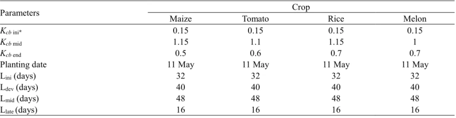
The crop parameters used as input for the soil water balance model IrrigRotation to estimate the IWR are presented in Table 2 (Vilar et al., 2015), in which the Kcb

values were empirically determined from the Kcb-NDVI

relationship (Equation 2) with the exception of Kcb ini, which was obtained from FAO 56, as

previously mentioned.

TABLE 2. Average crop parameters retrieved from EO data used to compute the IWR for the maize, tomato, rice and melon crops (adapted from Vilar et al., 2015).

Parameters Crop

Maize Tomato Rice Melon

Kcb ini* 0.15 0.15 0.15 0.15

Kcb mid 1.15 1.1 1.15 1

Kcb end 0.5 0.6 0.7 0.7

Planting date 11 May 11 May 11 May 11 May

Lini (days) 32 32 32 32

Ldev (days) 40 40 40 40

Lmid (days) 48 48 48 48

Llate (days) 16 16 16 16

* FAO 56 tabulated values.

The seasonal IWR computed for the selected crops are presented in Table 3, corresponding to the average of the crop parcels in the region. The standard deviation values resulting from the different soil types existing in the Vila Franca de Xira region are also listed.

TABLE 3. Average seasonal IWR (mm) for the rice, tomato, maize and melon crops (adapted from Vilar et al., 2015). Seasonal crop irrigation water requirements (mm)

Maize Tomato Rice Melon

average 639 611 835 587

standard deviation 15.1 15.3 0.2 26.4

TEST SITE II – VILA VELHA DE RÓDÃO

The second test site was in the Vila Velha de Ródão municipality, in the Castelo Branco district, east central Portugal (Figure 3). The main crops in the area are forage crops, maize, olive, permanent pasture and temporary pasture.

In this region, the climate according to the Köppen classification system is also Csa, i.e. a temperate climate with a hot and dry summer. Climate normal data, from 1971 to 2000, for the Castelo Branco weather station (39º 50’ N, 7º 28’ W, 386 m in altitude) of the IPMA network, show that the two hottest months are July and August, with monthly average temperatures higher than 24ºC, while winters are colder, with average temperatures lower than 10ºC from December to February. The highest monthly precipitation occurs in December (128.2 mm), while August is the driest month (8.4 mm). The average annual precipitation during the period of record is 758.3 mm.

This region was used by Rolim et al. (2016) to assess the use of both optical and Synthetic-Aperture Radar (SAR) data to estimate Kcb curves to be used for

IWR calculation. In that study, SPOT-5 Take-5 and Sentinel-1A data were used to generate, respectively, NDVI and backscattering time series for maize. Since a significant correlation between both data sets was found, a

preliminary empirical linear regression equation was proposed to estimate Kcb values from the SAR data,

demonstrating that SAR data might be useful to compute the IWR.

The developed methodology, in this study, was applied to site II to identify the eligible crop parcels, as well as to evaluate the use of optical images with higher spatial and temporal resolutions (SPOT-5 Take-5) to define the Kcb curves.

DATA

Earth Observation (EO) data

SPOT-5 Take-5 images acquired from April to September 2015 were used for site II. These images were provided by the Centre National d’ Études Spatiales (CNES) with a 10-m spatial resolution and 5-day revisit time. SPOT-5 Take-5 Level-2A images (orthorectified, bottom of atmosphere (BOA) reflectances) were used in this study because of their improved pre-processing level. Therefore, no further pre-processing steps were required. A total of 18 images without cloud cover were identified for the entire spring/summer crop growing season. The acquisition dates and the corresponding day of the year (DOY) are listed in Table 4.

TABLE 4. SPOT-5 Take-5 images acquisition dates for site II (DOY - Day of the Year, 2015 in this case).

Month Apr May Jun Jul Aug Sep

Day 13 23 28 18 23 28 17 22 27 2 7 12 22 27 1 11 26 10

RESULTS AND DISCUSSION

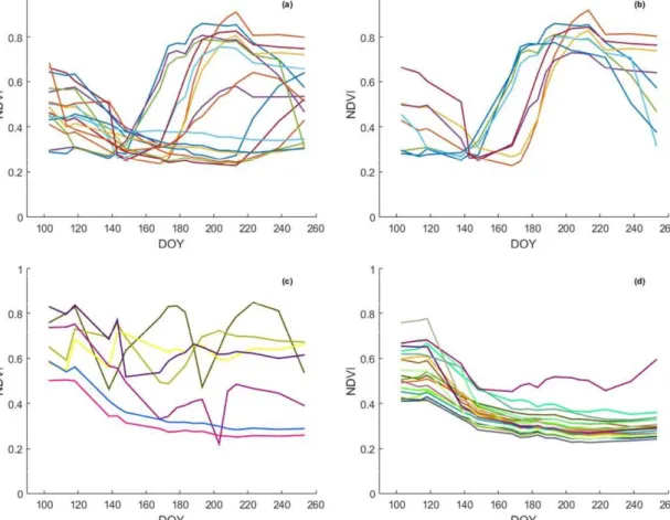
Using the set of curves approach, crop growth curves were generated for the main crops in the region. The average NDVI time series curves obtained for irrigated maize, irrigated pastures and non-irrigated meadow parcels are shown in Figure 6.

All parcels declared by the farmers as irrigated maize are plotted in Figure 6a, in which one can observe that some do not show the typical behaviour of this crop (Allen et al., 1998; Trout & DeJonge, 2018). After the removal of the outlier parcels, eight eligible maize parcels were obtained in which it was possible to identify, as shown in Figure 6b, different planting dates and lengths of the crop cycles. Therefore, it is demonstrated that it is possible to use NDVI time series with a short revisit time, 5 days in this case, to obtain better characterization of the crop growth cycle. Four parcels (sowed later) show an

anomalous behaviour during the late season (senescence), as well as an overestimation of the Kcb ini values (Rolim et

al., 2016). Both behaviours had already been observed for some parcels at site I, including for maize, using Landsat-8 data (Vilar et al., 2015). Ramme et al. (2010) also reported the occurrence of significant noise on crop NDVI temporal profiles, particularly for lower NDVI values because of the influence of soil and the need to filter the time series data. Uncertainties in the definition of the Kcb curve may also

result from the use of Kcb-NDVI empirical formulas

calibrated for other regions, and they should be validated for local conditions (D’Urso et al., 2010; Toureiro et al., 2017). However, despite these difficulties, the improved crop growth stages characterization, when using high spatial and temporal resolution satellite images such as SPOT5, is emphasized.

FIGURE 6. Mean NDVI time series for all parcels declared by the farmers as irrigated maize (a), after removing the outliers’ parcels (b), irrigated pasture parcels (c), and non-irrigated meadow parcels (d) at site II.

For irrigated pasture (Figure 6c), it is possible to detect several forage cuts given the short revisit time of the SPOT-5 Take-5 images. The NDVI curves obtained for the non-irrigated meadow parcels, shown in Figure 6d, reveal a very different pattern when compared to those obtained for the irrigated crops because of the effect of the high water stress of rainfed crops induced by the hot and dry summers characteristic of the Mediterranean climate.

Comparing these results to those obtained for site I, using Landsat-7 and -8 images, it is possible to conclude that the obtained Kcb curves are less accurate than those for

site II (SPOT5 Take-5) because of the reduced temporal resolution of the Landsat images. Therefore, it is

demonstrated that the use of EO data with higher spatial and temporal resolutions allows one to more reliably define detailed Kcb curves and consequently provide more

accurate IWR estimation. CONCLUSIONS

The proposed methodology was tested using the developed application software which proved to be suitable for the retrieval of crop data for IWR estimation at a regional level by providing accurate information relative to crop growth stages and crop coefficients. The determination of the Kcb curve using the EO-derived NDVI

time series allows for IWR estimation based on observations of the actual field crop growing conditions, and therefore, a more accurate soil water balance simulation is achieved.

This study demonstrated that the use of a single crop parcel or a small set of parcels may hamper crop behaviour characterization, particularly when the chosen parcel(s) is not representative of the crop pattern or of the management practices in the region. Considering a large sample of parcels for the estimation of crop parameters, it is possible to obtain a more representative and accurate crop coefficient curve, resulting in better ETc estimation.

It was observed that a denser EO time series enables better identification of the crop phenological stage lengths and planting/sowing dates and thus overcomes one of the major sources of uncertainty in IWR estimation. Although the results obtained using this methodology are encouraging, some difficulties were found mainly concerning the estimation of the initial and end of the late season Kcb values obtained using the Kcb-NDVI approach.

Caution should be exercised when using the Kcb-NDVI

empirical formulas, and field observations are required to validate the obtained results.

ACKNOWLEDGEMENTS

The authors would like to thank the IFAP for supplying the National Land Parcel Identification System (NLPIS) data for both municipalities. This publication was supported by FCT- project UID/GEO/50019/2019 - Instituto Dom Luiz.

REFERENCES

Allen RG, Pereira LS, Raes, D, Smith M (1998) Crop evapotranspiration: guidelines for computing crop water requirements. Rome, FAO, 300p. (Irrigation and Drainage Paper 56).

Allen RG, Tasumi M, Morse A, Trezza R (2007) Satellite-based energy balance for mapping evapotranspiration with internalized calibration (METRIC): Applications. Journal of Irrigation and Drainage Engineering 133(4):395-406. DOI:

https://doi.org/10.1061/(ASCE)0733-9437(2007)133:4(395)

Bastiaanssen WGM, Menenti M, Feddes RA, Holtslag AAM (1998) A remote sensing surface energy balance algorithm for land (SEBAL): 1 Formulation. Journal of Hydrology 212-213:198-212. DOI:

https://doi.org/10.1016/S0022-1694(98)00253-4 Calera Belmonte A, Jochum AM, Cuesta Garía A, Montoro Rodríguez A, López Fuster P (2005) Irrigation management from space: Towards user-friendly products. Irrigation and Drainage Systems 19:337-353. DOI: https://doi.org/10.1007/s10795-005-5197-x

Doorenbos J, Pruitt WO (1977) Guidelines for predicting crop water requirements. Rome, FAO, 144p. (Irrigation and Drainage Paper 24).

D’Urso G, Richter K, Calera A, Osann MA, Escadafal R, Garatuza-Pajan J, Hanich L, Perdigão A, Tapia JB, Vuolo F (2010) Earth Observation products for operational irrigation management in the context of the PLEIADeS project. Agricultural Water Management 98(2):271-282. DOI: https://doi.org/10.1016/j.agwat.2010.08.020 D’Urso G, Calera Belmonte A (2006) Operative approaches to determine crop water requirements from Earth Observation data: Methodologies and applications. In: Earth Observation for Vegetation Monitoring and Water Management, AIP Conference Proceedings 852:14-25. DOI: https://doi.org/10.1063/1.2349323

Du Y, Teillet PM, Cihlar J (2002) Radiometric

normalization of multitemporal high-resolution satellite images with quality control for land cover change

detection. Remote Sensing of Environment 82(1):123-134. DOI: https://doi.org/10.1016/S0034-4257(02)00029-9 El Hajj M, Bégué A, Guillaume S, Martiné J-F (2009) Integrating SPOT-5 time series, crop growth modeling and expert knowledge for monitoring agricultural practices: The case of sugarcane harvest on Reunion Island. Remote Sensing of Environment 113(10):2052-2061. DOI: https://doi.org/10.1016/j.rse.2009.04.009

Eldeiry AA, Waskom RM, Elhaddad A (2016) Using remote sensing to estimate evapotranspiration of irrigated crops under flood and sprinkler irrigation systems. Irrigation and Drainage 65(1):85-97 DOI:

https://doi.org/10.1002/ird.1945

Esquerdo J, Zullo Júnior J; Antunes J (2011) AVHRR time-series profiles for soybean crop monitoring in Brazil. International Journal of Remote Sensing 32(13):3711-3727. DOI: http://dx.doi.org/10.1080/01431161003764112 Ferreira E, Mannaersts CM, Dantas AA, Maathuis BH (2016) Surface energy balance system (SEBS) and satellite data for monitoring water consumption of irrigated sugarcane. Engenharia Agrícola 36(6):1176-1185. DOI:

http://dx.doi.org/10.1590/1809-4430-Eng.Agric.v36n6p1176-1185/2016

Grzegozewski DM, Uribe-Opazo MA, Johann JA, Guedes LPC (2017) Spatial correlation of soybean productivity, enhanced vegetation index (EVI) and agrometeorological variables. Engenharia Agrícola 37(3):541-555. DOI:

http://dx.doi.org/10.1590/1809-4430-eng.agric.v37n3p541-555/2017

Johann JA, Becker WR, Uribe-Opazo MA, Mercante E (2016) Uso de imagens do sensor orbital MODIS na estimação de datas do ciclo de desenvolvimento da cultura da soja para o estado do Paraná-Brasil. Engenharia Agrícola 36(1):126-142. DOI:

http://dx.doi.org/10.1590/1809-4430-Eng.Agric.v36n1p126-142/2016

Johann JA, Rocha, JV, Oliveira SRM, Rodrigues, LHA, Lamparelli RAC (2013) Data mining techniques for identification of spectrally homogeneous areas using NDVI temporal profiles of soybean crop. Engenharia Agrícola 33(3):511-524. DOI:

http://dx.doi.org/10.1590/S0100-69162013000300008 Navarro A, Rolim J, Miguel I, Catalão J, Silva J, Painho M, Vekerdy Z (2016) Crop Monitoring Based on SPOT-5 Take-5 and Sentinel-1A Data for the Estimation of Crop Water Requirements. Remote Sensing 8(6):525. DOI:

https://doi.org/10.3390/rs8060525

Neale CM, Bausch WC, Heerman DF (1989) Development of reflectance-based crop coefficients for corn.

Transactions of the ASAE 32(6):1891-1899. DOI:

https://doi.org/10.13031/2013.31240

Oliveira T, Ferreira E, Dantas A (2016) Temporal variation of normalized difference vegetation index (NDVI) and calculation of the crop coefficient (Kc) from NDVI in areas cultivated with irrigated soybean. Ciência Rural 46(9):1683-1688. DOI:

http://dx.doi.org/10.1590/0103-8478cr20150318 Paço TA, Pôças I, Cunha M, Silvestre JC, Santos FL, Paredes P, Pereira LS (2014) Evapotranspiration and crop coefficients for a super intensive olive orchard. An application of SIMDualKc and METRIC models using ground and satellite observations. Journal of Hydrology 519:2067-2080. DOI:

https://doi.org/10.1016/j.jhydrol.2014.09.075

Ramme FLP, Lamparelli RAC, Rocha JV (2010) Perfis temporais NDVI MODIS, na cana-soca, de maturação tardia. Engenharia Agrícola 30(3):480-494. DOI: http://dx.doi.org/10.1590/S0100-69162010000300012 Rolim J, Teixeira J (2008) IrrigRotation, a time continuous soil water balance model. WSEAS Transactions on Environment and Development 4(7):577-587.

Rolim J, Navarro A, Saraiva C, Catalão J (2016) A synergistic approach using optical and SAR data to estimate crop's irrigation requirements. Neale CM, Maltese, A (ed). In: Remote sensing for agriculture, ecosystems, and hydrology. Proceedings… DOI:

https://doi.org/10.1117/12.2241054

Rouse J, Haas R, Schell J, Deering D, Harlan J (1974) Monitoring the vernal advancement of retrogradation of natural vegetation, Type III, Final Report. Greenbelt: NASA/GSFC.

Toureiro C, Serralheiro R, Shahidian S, Sousa A (2017) Irrigation management with remote sensing: Evaluating irrigation requirement for maize under Mediterranean climate condition. Agricultural Water Management 184:211-220. DOI:

https://doi.org/10.1016/j.agwat.2016.02.010

Trout T, DeJonge K (2018) Crop water use and crop coefficients of maize in the great plains. Journal of Irrigation and Drainage Engineering 144(6):04018009. DOI: 10.1061/(ASCE)IR.1943-4774.0001309

Vilar P (2015) Utilização de imagens de detecção remota para monitorização das culturas e estimação das

necessidades de rega. Dissertação Mestrado, Lisboa, Faculdade de Ciências da Universidade de Lisboa. Vilar P, Navarro A, Rolim J (2015) Utilização de imagens de deteção remota para monitorização das culturas e estimação das necessidades de rega. In: Conferência Nacional de Cartografia e Geodesia, Lisboa, Proceedings... Vuolo F, D’Urso G, De Michele C, Bianchi B, Cutting M (2015) Satellite-based irrigation advisory services: A common tool for different experiences from Europe to Australia. Agricultural Water Management 147:82-95. DOI: https://doi.org/10.1016/j.agwat.2014.08.004