Can fire spread simulations contribute to support decisions in a fire suppression context ? An evaluation using MaxEnt, FARSITE and satellite active fire data

(1)

Can fire spread simulations contribute to support

decisions in a fire suppression context?

An evaluation using MaxEnt, FARSITE and satellite active fire data.

Rafael Coelho Baptista

Dissertação para a obtenção do grau de mestre em

Engenharia Florestal e dos Recursos Naturais

Orientadores: Doutora Ana Cristina Lopes de Sá

Doutor José Miguel Cardoso Pereira

Júri:

Presidente:

Doutora Maria da Conceição Brálio de Brito Caldeira, Professora Auxiliar, Instituto Superior de Agronomia

Vogais:

Doutor José Miguel Oliveira Cardoso Pereira, Professor Catedrático, Instituto Superior de Agronomia

Doutor João Manuel das Neves Silva, Investigador Integrado, Fundação para a Ciência e Tecnologia.

(2)

Abstract

This work is of an exploratory nature and describes and evaluates a method to simulate fire spread which, in an operational context, has the potential to be used as a decision-support tool for fire management and suppression.

The use of fire spread models has, for the most part, followed a deterministic approach, which does not account for predictions uncertainty. However, fire spread models are subject to assumptions and limitations that inherently produce errors during simulations and so should be integrated in the simulations themselves. For that matter uncertainty was propagated through Farsite fire behavior model by randomly defining 100 different independent combinations of some of the most important input variables. The simulations were run with three different fuel maps, one standardized and two customized.

For the evaluation of the fire spread predictions a qualitative and a quantitative analysis were made. Both analyses used MaxEnt derived reference perimeters, and active fire data was used on the qualitative analyses to add temporal depth to the evaluation.

Results showed that uncertainties in wind speed and direction, location of ignitions (spatial and temporal), fuel model assignment and typology may have major impact on prediction accuracy. Overall, fuel models presented better results when compared with the standard model and generally showed higher Kappa and burned class agreement values and lower omission errors. This thesis suggests that this method has major potential to optimize fuel management practices, especially if simulations are run with fuel maps derived Portuguese landcover maps.

(3)

Resumo

Esta tese é de natureza exploratória e descreve e avalia um método para simular a propagação de fogo.

A utilização de modelos que simulam a propagação de fogo tem, em grande parte, seguido uma abordagem determinística, que não tem em conta a incerteza das previsões. No entanto os modelos de propagação de fogo estão sujeitos a pressupostos e limitações que inerentemente produzem erros durante as simulações e deviam por isso ser integrados nas previsões. Propõe-se, para esse efeito, a aferição das previsões probabilísticas de doze fogos com áreas ardidas superiores a 500 ha ocorridos na região centro-norte de Portugal no ano de 2015, integrando a incerteza de algumas das variáveis de input nessas previsões.

Para simular a propagação dos fogos foi utilizado o simulador FARSITE e a incerteza foi propagada definindo aleatoriamente combinações independentes de 100 para os parâmetros e variáveis de input: ignição, vento e humidade relativa. As simulações foram corridas com três mapas de combustível diferentes, um standard e dois customizados.

.Para a avaliação das previsões de propagação do fogo foram feitas uma análise qualitativa e uma quantitativa. Ambas fizeram uso de perímetros de referência derivados do classificador MaxEnt. Foram também utilizados dados térmicos de satélite de modo a adicionar uma dimensão temporal à avaliação qualitativa.

Os resultados mostram que a incerteza relacionada com a velocidade e direção do vento, localização (temporal e espacial) das ignições

No geral, as previsões corridas com os mapas de combustivel costumizados apresentaram resultados melhores quando comparados com os mapas standard, apresentando valores de Kappa e Burnt Class Agreement mais elevados e erros por omição mais baixos. Esta tese sugere que este metodo de simulação da propagação de fogo tem um grande potencial para otimizar a gestão e combate do fogo, especialmente quando utilizados os mapas de combustível derivados de mapas de ocupação do solo Portugueses.

(4)

Resumo alargado

Esta tese é de natureza exploratória e descreve e avalia um método para simular a propagação de fogo que, num contexto operacional, têm potencial de ser utilizado como ferramenta de apoio à decisão em operações de gestão e combate do fogo.

A utilização de modelos que simulam a propagação de fogo tem, em grande parte, seguido uma abordagem determinística, que não tem em conta a incerteza das previsões. No entanto os modelos de propagação de fogo estão sujeitos a pressupostos e limitações que inerentemente produzem erros durante as simulações e deviam por isso ser integradas nas previsões. Propõe-se, para esse efeito, a aferição das previsões probabilísticas de doze fogos com áreas ardidas superiores a 500 ha ocorridos na região centro-norte de Portugal no ano de 2015, integrando a incerteza de algumas das variáveis de input nessas previsões.

Para simular a propagação dos fogos foi utilizado o simulador FARSITE por ser um modelo temporal e espacialmente explicito sendo, portanto, capaz de produzir previsões detalhas. A incerteza foi propagada definindo aleatoriamente combinações independentes de 100 para os parâmetros e variáveis de input: ignição, vento e humidade relativa.

Para cada caso de estudo as simulações de propagação do fogo foram executadas com mapas de combustível standard e customizados. O mapa standard foi criado traduzindo as classes de ocupação do solo da CORINE em classes de combustível de acordo com a os serviços florestais norte-Americanos e os modelos customizados foram criados traduzindo classes de ocupação do solo da CORINE em classes de combustível customizadas e classes de ocupação do solo dos serviços florestais Portugueses em classes de combustível customizadas.

Foram utilizadas duas abordagens distintas para avaliar a precisão das simulações, uma qualitativa e outra quantitativa, usando dados térmicos de satélite na última. A analise qualitativa das simulações foi feita comparando os mapas de previsão de propagação do fogo com perímetros de referência e com dados térmicos de satélite adicionando uma dimensão temporal à avaliação. Os perímetros de referência com os quais as previsões foram comparadas foram obtidos por meio do classificador MaxEnt. Imagens Landsat foram utilizadas para retirar áreas de treino para input no classificador, alguns índices de vegetação foram também utilizados como input de modo a melhorar os outputs do classificador.

Os dados térmicos de satélite foram também utilizados para definir ignições e datas de inicio e fim de alguns dos casos de estudo e foram comparados com as progressões de algumas das melhores simulações de modo a aperfeiçoar a avaliação.

As previsões de propagação do fogo foram avaliadas quantitativamente procedendo a elaboração de matrizes fruto de comparações binarias entre os mapas probabilísticos de propagação do fogo e os perímetros de referência. Baseadas nessas matrizes foram

(5)

calculadas: a tendência relativa (RelB), o Kappa de Coen, concordância entre as classes “burned” (ardido, BCA), o erro geral (DP), e os erros de omissão (OE) e comissão (CE) para cada uma das 36 previsões.

São apresentados os resultados das simulações de todos os casos de estudo corridas com os três mapas de combustível, mas apenas as previsões obtidas usando os modelos de combustível customizados são discutidas dada a qualidade inferior das simulações quando corridas com o modelo standard. A discussão foi limitada a seis casos de estudo, que foram considerados representativos do todo, cobrindo um leque alargado de assuntos.

Do ponto de vista qualitativo, as previsões dos casos de estudo de Mangualde da Serra, Sá e Valdosende mostraram bons resultados, e uma razoável correspondência entre as simulações de propagação do fogo e os respetivos perímetros de referência. As

simulações dos casos de Candemil, Espadanedo e Lavandeira apresentaram resultados comparativamente piores, ainda assim, foi possível extrair informação relevante a cerca de como algumas das variáveis de input influenciam as previsões de propagação do fogo. As restantes previsões subestimaram claramente a progressão do fogo, não mostrando qualquer direção dominante de progressão.

Ambas a simulações do caso de estudo de Sá corridas com os modelos

customizados, mostraram uma boa correspondência com os respetivos dados térmicos de satélite. O caso de estudo de Mangualde da Sera, ainda que atrasado nas primeiras horas quando comparado com os dados térmicos, acabou por sobrestimar a progressão do fogo independentemente do mapa de combustível utilizado. Do mesmo modo o caso de estudo de Valdosende ultrapassou as posições dos fogos ativos sobrestimando sobretudo na fronteira sul. A simulação do caso de Lavandeira em que foi utilizado o modelo de

combustível customizado traduzido da carta de ocupação do solo portuguesa, apresar da forma complexa do seu perímetro, teve os seus contornos simulados bastante bem, mas apenas simulou 60% da área ardida de referência. Tal como esta previsão, a maior parte, 26 das 36 previsões, subestimaram a progressão do fogo pelo menos numa frente.

De um modo geral, as simulações corridas com os modelos customizados apresentaram resultados melhores, o que está de acordo com a análise quantitativa que apresenta valores de Kappa e BCA mais elevados e valores de OE mais baixos para as simulações corridas com estes modelos. Ainda assim foram encontradas algumas

discrepâncias entre a análise qualitativa e a quantitativa. O RelB revelou a tendência que as simulações têm em sobrestimar a progressão do fogo, mesmo em casos onde foi observada subestimação, tal como são exemplo as previsões dos casos de Candemil e Graça em que foram utilizados modelos de combustível customizados traduzidos da carta de ocupação da

(6)

CORINE. Ainda que a analise qualitativa depreenda que existe subestimação na fronteira sul, os seu valores de RelB estão ambos acima de 1.

Nenhum valor de Kappa foi igual a 1, e foram obtidos valores abaixo de 0 para algumas das previsões. Os valores mais elevados de Kappa foram de 0.5 e 0.4.

O índice BCA revelou resultados bastante bons para alguns dos casos de estudo. Foram registados valores de 100% e 99% para as previsões de Mangualde da Serra e Sá respetivamente. Ainda assim foram registados valores bastante baixos para as previsões Mangualde e Alvaro, 8.5% e 12.8% respetivamente.

No que diz respeito aos OE, as previsões de propagação de fogo para o caso de estudo de Mangualde da Serra e Sá tiveram valores abaixo da referência “ideal” (4.4%). As previsões para o caso de Valdosende tiveram valores abaixo da referência “razoável” (13%). As restantes têm valores acima da referência “máxima”, com as previsões dos casos de Alvaro e Mangualde a ter valores de 99% e 92% respetivamente. Cinco casos de estudo tiveram valores de DP a baixo da referência “máxima” (25%). As restantes tiveram valores acima dessa referência com máximos de 53% e 51% para as previsões Mangualde da Serra e Valdosende respetivamente.

Em última análise, o FARSITE foi capaz de apresentar bons resultados para alguns dos casos de estudo analisados e a precisão das simulações revelou-se de um modo geral superior quando utilizado o mapa de combustível traduzido do COS. Ainda assim outras tantas simulações tiveram resultados aquém do operacionalmente vantajoso. A incorreta representação da direção e velocidade do vento e a sua resolução espacial, cartas de ocupação do solo desatualizadas, localização errada das simulações e não simular a propagação do fogo através de spotting têm os maiores impactos na incorreta

representação da propagação do fogo. Ainda que as previsões com bons resultado sejam indubitavelmente uteis, num contexto operacional não existiria maneira de as distinguir de representações incorretas.

Palavras-chave: simulações probabilisticas, fogos activos, MaxEnt

(7)

Index

List of figures List of tables

List of abbreviations

1.Introduction ... 1

2.Data and Methods ... 4

2.1. Study area ... 4

2.2. Satellite data ... 5

2.3. Fire Reference Perimeters ... 6

2.4.Fire spread simulations ... 6

2.4.1. Data requirements ... 7

2.4.1. Uncertainty quantification ... 8

2.5. Qualitative and quantitative analyses ... 8

3.Results ... 11

4.Discution ... 36

5.Conclusion ... 47

References ... 48

(8)

List of Figures

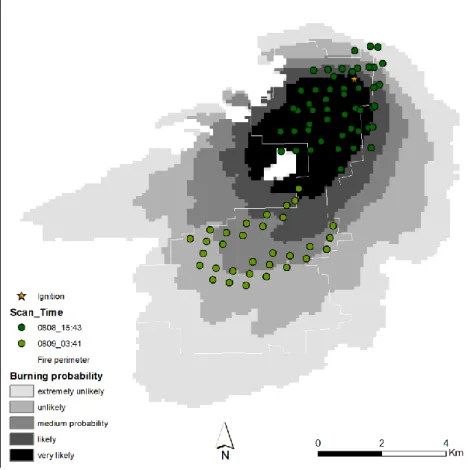
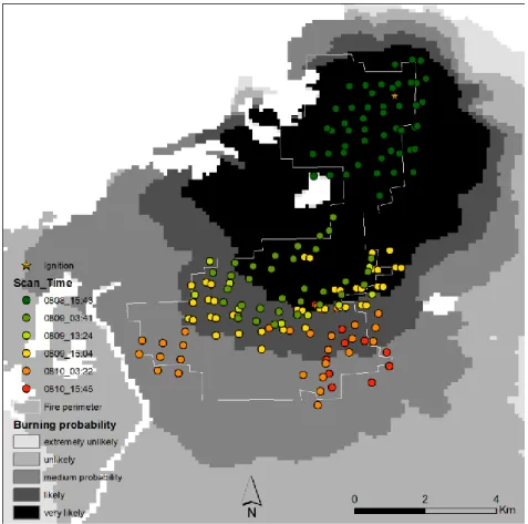
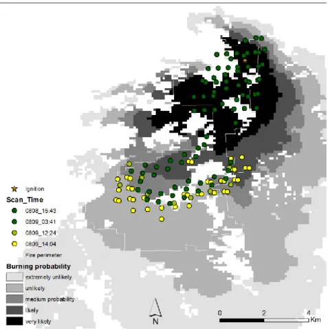
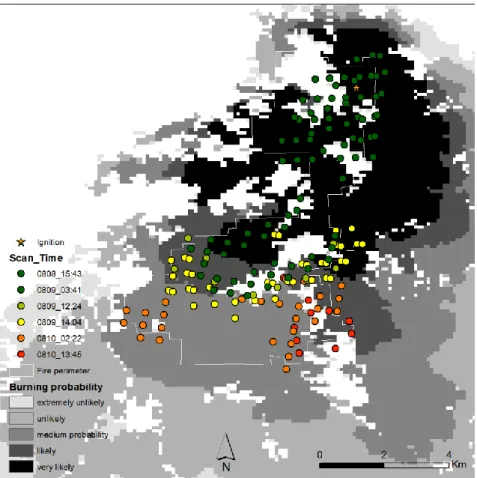
Fig. 1 – RGB composite of the study area made with the Landsat 8 images (band 5,4,3) for October 2015, borders of the reference perimeters highlighted in red; HRL for the area obstructed by the clouds (left corner) ...4 Fig. 2 – Fire spread simulations for ASTM(A1), ACM1(A2) and ACM2(A3) are presented in grey shading according to burning probability. Reference perimeters are presented in red ... 12 Fig. 3 – Fire spread simulations for BSTM(B1), BCM1(B2) and BCM2(B3) are presented in grey shading according to burning probability. Reference perimeters are presented in red ... 13 Fig. 4 – Active fires for BCM1 6h after ignition represented in green. Respective fire spread simulation in grey shading ... 13 Fig. 5 – Active fires for BCM1 16h after ignition represented in a colour gradient. Respective fire spread simulation in grey shading ... 14 Fig. 6 – Active fires for BCM1 26h after ignition represented in a colour gradient. Respective fire spread simulation in grey shading ... 14 Fig. 7 – Active fires for BCM1 28h after ignition represented in a colour gradient. Respective fire spread simulation in grey shading ... 15 Fig. 8 – Active fires for BCM1 40h after ignition represented in a colour gradient. Respective fire spread simulation in grey shading ... 15 Fig. 9 – Active fires for BCM1 51h after ignition represented in a colour gradient. Respective fire spread simulation in grey shading ... 16 Fig. 10 – Active fires for BCM2 6h after ignition represented in green. Respective fire spread simulation in grey shading ... 16 Fig. 11 – Active fires for BCM2 16h after ignition represented in a colour gradient. Respective fire spread simulation in gray shading ... 17 Fig. 12 – Active fires for BCM2 26h after ignition represented in a colour gradient. Respective fire spread simulation in grey shading ... 17 Fig. 13 – Active fires for BCM2 28h after ignition represented in a colour gradient. Respective fire spread simulation ... 18 Fig. 14 – Active fires for BCM2 40h after ignition represented in a colour gradient. Respective fire spread simulation in grey shading ... 18 Fig. 15 – Active fires for BCM2 51h after ignition represented in a colour gradient. Respective fire spread simulation in grey shading ... 19 Fig. 16 – Fire spread simulations for CSTM(C1), CCM1(C2) and CCM2(C3) are presented in grey shading according to burning probability. Reference perimeters are presented in red... 19 Fig. 17 – Fire spread simulations for DSTM(D1), DCM1(D2) and DCM2(D3) are presented in grey shading according to burning probability. Reference perimeters are presented in red... 20 Fig. 18 – Fire spread simulations for ESTM(E1), ECM1(E2) and ECM2(E3) are presented in grey shading according to burning probability. Reference perimeters are presented in red... 20

(9)

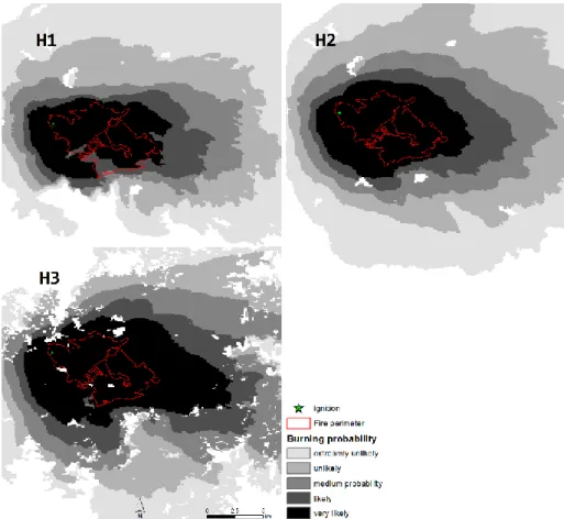
Fig. 19 – Fire spread simulations for FSTM(F1), FCM1(F2) and FCM2(F3) are presented in grey shading according to burning probability. Reference perimeters are presented in red ... 21 Fig. 20 – Fire spread simulations for GSTM(G1), GCM1(G2) and GCM2(G3) are presented in grey shading according to burning probability. Reference perimeters are presented in red. ... 21 Fig. 21 – Fire spread simulations for HSTM(H1), HCM1(H2) and HCM2(H3) are presented in grey shading according to burning probability. Reference perimeters are presented in red. ... 22 Fig. 22 – Active fires for HCM1 13h after ignition represented in green. Respective fire spread simulation in grey shading ... 22 Fig. 23 – Active fires for HCM1 14h after ignition represented in a colour gradient. Respective fire spread simulation in grey shading ... 23 Fig. 24 – Active fires for HCM1 24h after ignition represented in a colour gradient. Respective fire spread simulation in grey shading ... 23 Fig. 25 – Active fires for HCM1 36h after ignition represented in a colour gradient. Respective fire spread simulation in grey shading ... 24 Fig. 26 – Active fires for HCM1 38h after ignition represented in a colour gradient. Respective fire spread simulation in grey shading ... 24 Fig. 27 – Active fires for HCM1 60h after ignition represented in a colour gradient. Respective fire spread simulation in grey shading ... 25 Fig. 28 – Active fires for HCM2 13h after ignition represented in green. Respective fire spread simulation in grey shading ... 25 Fig. 29 – Active fires for HCM2 14h after ignition represented in a colour gradient. Respective fire spread simulation in grey shading ... 26 Fig. 30 – Active fires for HCM2 24h after ignition represented in a colour gradient. Respective fire spread simulation in grey shading ... 26 Figure 31 – Active fires for HCM2 36h after ignition represented in a colour gradient. Respective fire spread simulation in grey shading ... 27 Figure 32 – Active fires for HCM2 38h after ignition represented in a colour gradient. Respective fire spread simulation in grey shading ... 27 Fig. 33 – Active fires for HCM2 60h after ignition represented in a colour gradient. Respective fire spread simulation in grey shading ... 28 Fig. 34 – Fire spread simulations for ISTM(I1), ICM1(I2) and ICM2(I3) are presented in grey shading according to burning probability. Reference perimeters are presented in red ... 28 Fig. 35 – Fire spread simulations for JSTM(J1), JCM1(J2) and JCM2(J3) are presented in grey shading according to burning probability. Reference perimeters are presented in red ... 29 Fig. 36 – Active fires for JCM1 4h after ignition represented in green. Respective fire spread simulation in grey shading ... 29 Fig. 37 – Active fires for JCM1 13h after ignition represented in a colour gradient. Respective fire spread simulation in grey shading ... 30 Fig. 38 – Active fires for JCM1 15h after ignition represented in a colour gradient. Respective fire spread simulation in grey shading ... 30

(10)

Fig. 39 – Active fires for JCM1 18h after ignition represented in a colour gradient. Respective fire spread simulation in grey shading ... 31 Fig. 40 - Active fires for JCM1 38h after ignition represented in a colour gradient. Respective fire spread simulation in grey shading ... 31 Fig. 41 - Active fires for JCM2 4h after ignition represented in green. Respective fire spread simulation in grey shading ... 32 Fig. 42 – Active fires for JCM2 13h after ignition represented in a colour gradient. Respective fire spread simulation in grey shading ... 32 Fig. 43 – Active fires for JCM2 15h after ignition represented in a colour gradient. Respective fire spread simulation in grey shading ... 33 Fig. 44 - Active fires for JCM2 28h after ignition represented in a colour gradient. Respective fire spread simulation in grey shading ... 33 Fig. 45 – Active fires for JCM2 38h after ignition represented in a colour gradient. Respective fire spread simulation in grey shading ... 34 Fig. 46 – Fire spread simulations for KSTM(K1), KCM1(K2) and KCM2(K3) are presented in grey shading according to burning probability. Reference perimeters are presented in red... 34 Fig. 47 – Fire spread simulations for LSTM(L1), LCM1(L2) and LCM2(L3) are presented in grey shading according to burning probability. Reference perimeters are presented in red. ... 35 Fig. 48 – Fuel models for KCM1 (left) and KCM2 (right) with each fuel class represented by a different colour (fuel model classes described in Table 6), “very likely” class in black and reference perimeter in yellow ... 38 Fig. 49 – Cumulative wind direction histogram (left) and wind speed graphic (right) computed with the weather information used for the simulations of case study K. ... 38 Fig. 50 – Modis aqua for 22th of August (≈12h after ignition) overlaid with the simulation for KCM2 in grey shading and corresponding reference perimeter in red and ignition in green ... 39 Fig. 51 – Google Earth image with the reference perimeter shaded in red and a road highlighted in blue

... 39 Fig. 52 – Fuel models for BCM1 (left) and BCM2 (right) with each fuel class represented by a different color (fuel model classes described in Table 6), “very likely” class in black and reference perimeter in yellow ... 40 Fig. 53 – Cumulative wind direction histogram (left) and wind speed graphic (right) computed with the weather information used for the simulations of case study B ... 40 Fig. 54 – Fuel models for FCM1 and FCM2 with each fuel class represented by a different colour (fuel model classes described in Table 6), “very likely” class in black and reference perimeter in yellow .... 41 Fig. 55 – Fuel models for GCM1 and GCM2 with each fuel class represented by a different colour (fuel models described in Table 6), “very likely” class in black and reference perimeter in yellow ... 42 Fig. 56 – Fuel models for JCM1 (left) and JCM2 (right) with each fuel class represented by a different color, respectively and corresponding “very likely” class in black and reference perimeter in yellow. Numbers in the legend correspond to the descriptions in table ... 42

(11)

Fig. 57 – Cumulative wind direction histogram (left) and wind speed graphic (right) computed with the weather information used for the simulations of case study J ... 43 Fig. 58 – Google Earth image with the reference perimeter for case study J shaded in red and a road highlighted in blue ... 43 Fig. 59 – Google Earth image with the reference perimeter for case study J shaded in red and a road highlighted in blue ... 44 Fig. 60 – RGB composite of case H, ignition in white and Penhas Douradas weather station in blue . 44 Fig. 61 – Wind speed graphic computed with the weather information used for the simulations of case study H and Penhas Douradas weather station data ... 45 Fig. 62 – RGB close up of the road/fire containment line present in the reference perimeter of case study H ... 45 Fig. 63 – HRL aqua from the 10th of August (24h), the contours of the HCM2 simulation and respective reference perimeter ... 46 Fig. 64 – Cumulative wind direction histogram computed with the weather information used for the simulations of case study H and Penhas Douradas weather station data ... 46 Fig. 65 – Fuel models for HCM1 and HCM2 with each fuel class represented by a different colour (fuel models described in Table 6), “very likely” class in black and reference perimeter in yellow ... 46 Fig. 66 – Google Earth closeup to the west flank. Burnt scar area shaded in red. Roads in blue .. 47 Fig. 67 – Google Earth closeup to the southwest flank. Burnt scar area shaded in red. Roads in blue47

(12)

List of Tables

Table 1 Case studies with respective identification codes, ignitions, alert date, duration and both the

areas of the reference perimeters of the ones provided by ICNF ... 5

Table 2 – Landsat 8 bands designation and wavelength ... 7

Table 3 – Predictions’ probability classes ... 8

Table 4 – Confusion matrix between reference and simulated data ... 10

Table 5 – Calculated statistics, the values in dark green are the best values for each statistic, in lighter green are within their respective thresholds, in red the lowest values and in yellow other relevant values ... 36

(13)

Abbreviations

BA - Burned Area

BCA – Burned Class Agreement CE – Commission Error

CEF - Centro de Estudos Florestais CLC - CORINE Land Cover

COS – Cartografia de Ocupação do Solo DP – Disagreement Proportion

EDC - Data Center

EROS - Earth Resources Observation Systems ESA - European Space Agency

FARSITE - Fire Area Simulator GIS - Geographic Information System HRL - High Resolution Layers

ICNF – Instituto da Conservação da Natureza e das Florestas Kappa – Cohen’s Kappa Statistic

MODIS - Moderate Resolution Imaging Spectroradiometer NASA - National Aeronautics and Space Administration NDVI - Normalized Difference Vegetation Index

NFFL – National Forest Fire Laboratory OE – Omission Error

OLI - Operational Land Imager

PTFM – Portuguese custom Fuel Models RelB – Relative Bias

RGB – Composite where: R=red, G=green B=blue SRTM - Shuttle Radar Topography Mission TIRS - Thermal InfraRed Sensor

USGS - United States Geological Survey

VIIRS – Visible Infrared Imaging Radiometer Suite WRF - Weather Research and Forecasting

(14)

1

1. Introduction

The Mediterranean region is a fire-prone area with the highest fire incidence in Europe (Turco et al. 2016). Some studies have identified an increasing fire risk specially for Portugal (Pereira et al. 2013; Turco et al. 2016). In the last forty years the country suffered socio-economic and demographic changes, which led to rural abandonment and consequently to the accumulation of biomass and to the neglect of agricultural practices that shaped a structural mosaic. This promoted shrub encroachment and increased the Portuguese landscape-level flammability (Costa et al. 2010; Marques et al. 2011; Fernandes et al. 2014).

Although it is in the most densely populated areas where the greatest number of fires occur, the demographic and ecological conditions of such areas do not favor large fires. It is in the rural areas, that have undergone very sharp eco sociological changes, altering the eco-biogeographical conditions, where there are larger fires.

The largest fires tend to occur under more severe heat, drought and wind conditions. These conditions promote the spread of fires even through areas with low fuel loads or with more vegetation moisture content. Future climatic scenarios point to an increase in temperatures in spring and summer and more frequent heat waves, these combined with strong favorable winds, will likely lead to extensive and more severe fire seasons (Ramos et al. 2011).

The Portuguese fire suppression capabilities are exceeded by the more intensive and frequent wildfires likely to occur under those extreme weather conditions. The detection and suppression system can extinguish most of the ignitions during its first moments, however the remaining cause the largest damage. During the 2003 fire season, 1% of the fires were responsible for 90% of the burned area of that year (Pereira et al. 2005). Extreme weather conditions were recorded with a devastating sequence of large wildfires resulting in ca. 440,000 ha of total burned area, approximately twice the previous highest record (220,000 ha in 1998) (Trigo et al. 2006). In 2005, as a consequence of one of the longest and most severe droughts of the last century, a total of 340,000 ha burned, making it the second worst burned area record at the time. More recently, 2017 had the maximum record of burned area extent 442,418 ha (ICNF, 2017)

The context above mentioned highlights the importance of studying and modeling fire spread as a spatial phenomenon to support landscape and fire management decisions, aiming at anticipating and minimizing the impacts of large wildfires. Fire spread models are an effective tool to study interactions between the main drivers of fire behavior — meteorological conditions, topography and vegetation (Keane et al. 2004), and have been widely used to simulate fire spread for prospective fuel treatment planning (Salis et al., 2016a), informing

(15)

real-2

time suppression decision-making (Calkin et al., ;Salis et al. 2016b), assessing wildfire risk to a variety of resources (Hollingsworth et al. 2012 ) and ultimately for education and training.

The FARSITE (Fire Area Simulator, Finney 1998) is one of the main fire simulation systems developed to describe the fire spread and behavior properties. As a spatially and temporally explicit model, FARSITE can produce detailed simulations of fire behavior and provide additional information such as fire rate of spread, fire-line intensity, among other fire descriptors. It requires the support of a GIS system, to generate and provide spatial data regarding fuels vegetation, and topography (Cochrane et al., 2012). The characteristics of the vegetation are approximated using a set of standard or customized fuel models (Anderson 1982, Fernandes 2005).

A fuel model is an association of forest fuel components of distinctive species, form, size, arrangement and continuity that will exhibit a characteristic behavior under defined burning conditions (Anderson 1982). The standard fuel models were designed for US fuel types, making extrapolation to other ecosystems not always reliable and can result in biased outputs (Arca et al. 2007). For these reasons much effort has been dedicated to developing alternatives to standard fuel models, with customized fuel models being developed more recently to better represent the fuel characteristics of the Portuguese vegetation (Fernandes et al. 2001, Cruz and Fernandes 2008)

Modeling fire behavior is subject to limitations that produce errors in simulations (Alexander and Cruz 2013; Hilton et al. 2015) making it important to consider uncertainty associated with model input variables and parameters when supporting fire planning and suppression (Thompson and Calkin 2011; Pacheco et al. 2015; Banali et al. 2016). Several works have integrated the uncertainty in fire spread modelling, using probabilistic approaches (Cruz 2010; Calkin et al. 2011; Finney et al. 2011a, b; Hilton et al. 2015, Benali et al. 2016, Pinto at al. 2016) Still, in an operational context the use of fire spread models has, for the most part, followed a deterministic approach (Cruz and Alexander 2013), ignoring data uncertainty in their predictions. Although fire spread predictions become more accurate if the uncertainty associated with model input variables and parameters are integrated in model predictions (Benali, 2016), it also makes fire more difficult to predict (Thompson and Calkin 2011) due to computational constraints, information on wind and fuel variability and knowledge of the dynamic interactions between fire and its environment (Alexander and Cruz, 2013; Hilton et al., 2015).

The main purpose of this thesis is to understand how reliable fire spread predictions are by evaluating the accuracy of the fire spread predictions performed with standard and customized fuel models. For that, we propose to assess: the probabilistic predictions of fire spread during some of the biggest fires (> 500 ha) of 2015 integrating the uncertainty of input

(16)

3

variables; and the potential of these simulations as a decision-support tool for fire suppression in an operational setting.

For this purpose, we used the FARSITE simulator to predict the spread of a set of wildfires that occurred along the north-central region of Portugal. Then, we analyzed the effects of fuel models, wind and other variables on predictions’ accuracy.

(17)

4

2. Data and methods

2.1. Study area

We proposed to simulate fires with burnt area extents greater than 500 ha in the central-north region of Portugal for the year of 2015 (Fig.1). As meteorological data was only available from the 23rd_{of July onwards, we simulated only 12 out of 24 cases (Table 1). The northern}

region is characterized by a large occupation by forest (38%) and agriculture (28%) and the largest effective shrub area (23%, Caetano et al 2017). According to Instituto Português do Mar e da Atmosfera (IPMA) the month the whole month of August 2015 – when 11 out of the 12 fires occurred – was generally dry. Not only for Viana do Castelo and Braga which had cumulative precipitation values of 24.9mm and 45.8mm respectively. Temperatures ranged from 7.6 ºC (on the 14th_{) and 38ºC (10}th_{) and the mean values for maximum and minimum}

Fig. 1 – RGB composite of the study area made with the Landsat 8 images (bands 5, 4 and 3) for October 2015, borders of the reference perimeters highlighted in red; Modis aqua for the area

(18)

5

Table 1 Case studies with respective identification codes, ignitions, alert date, duration and both the areas of the reference perimeters of the ones provided by ICNF

Civil Perish CLC-NFFL code CLC-PTFM code COS-PTFM code Ignition (lat) Ignition (long) Date Alert Hour Alert Duration Area ICNF Area Ref. Per.

Álvaro ASTM ACM1 ACM2 39.966 -7.967 08/03 13:43 13h 777 714

Candemil BSTM BCM1 BCM2 41.934 -8.711 08/08 10:54 51h 3024 2649

Casteleiro CSTM CCM1 CCM2 40.277 -7.304 08/02 16:23 21h 1190 1127

Espadanedo DSTM DCM1 DCM2 41.646 -6.911 08/30 17:02 10h 570 406

Graça ESTM ECM1 ECM2 39.922 -8.256 08/06 14:00 24h 550 465

Lavandeira FSTM FCM1 FCM2 41.171 -7.284 07/26 12:27 16h 520 477

Mangualde GSTM GCM1 GCM2 40.579 -7.766 08/10 12:20 17h 761 565

Mangualde da Serra HSTM HCM1 HCM2 40.455 -7.602 08/10 14:44 60h 2557 2337

Povoa de Cervães ISTM ICM1 ICM2 40.569 -7.692 08/06 15:59 15h 985 937

Sá JSTM JCM1 JCM2 42.068 -8.344 08/08 22:56 38h 1105 952

Sortelha KSTM KCM1 KCM2 40.337 -7.244 08/22 02:36 26h 4673 4995

(19)

6

temperatures were 27.7 and 14.3 ºC, respectively. Maximum registered wind speed of 61.2 and 58.3 Km/h in Guarda (on the 30th_{) and Viseu (on the 23}rd_{), respectively}

2.2. Satellite data

The Landsat 8 images (203 31, 203 32, 204 31 and 204 32, Fig.1) for the 10th_{of October}

2015 were downloaded from the Earth Resources Observation Systems (EROS) Data Center (EDC) of the USGS (http://glovis.usgs.gov). They were used to make the RGB composites from which the training areas for the reference fire perimeters were taken. The images come in GeoTIFF data format, with 16-bit pixel values, OLI multispectral bands 1-7,9 with 30m spatial resolution, OLI panchromatic band 8 with 15 m, TIRS bands 10-11 collected at 100 m but resampled to 30 m to match OLI multispectral bands.

Although the quality of satellite active fire data is dependent on multiple factors such as revisit cycle, viewing geometry, fire size, duration and intensity, thermal contrast between the fires and the surrounding areas, cloud clover, etc. (Giglio 2010, Olivia and Schroeder 2015), active fires can systematically provide information on the spatial dynamics of wildfires thus being able to function as an evaluation tool (Sa et al., 2016).

We used active fire data from MODIS (MCD14ML) and VIIRS 375, which combine the middle-infrared and the thermal bands to identify active fires and separate them from fire-free background, to discriminate clouds, sun glint, and water bodies. They provide information about the location, date, and time of the detected active fires and are acquired on every six hours (average four times per day) for MODIS and twelve hours (average two times per day) for VIIRS, with a nominal spatial resolution of 1000 and 375m2, respectively (Giglio 2010; Schroeder et al. 2014, Olivia and Schroeder 2015).

They were used to determine fire event duration, evaluate temporal and spatial discrepancies between active fire's observations and simulated fire growth and to set ignition locations as 8 out of the 12 were outside the reference fire perimeter. The locations of the first active-fires detected were set as the ignition points for some simulations. And for some cases the last active fires detected over the reference fire perimeter were extracted to determine the end date. We ended up relying more on MODIS do set ignitions and end dates due to its higher frequency and on VIIRS for the qualitative analyses to its higher spatial resolution.

(20)

7

2.3. Fire reference perimeters

The reference perimeters to which the simulations were compared were derived from four RGB composites, and MaxEnt classifier (Phillips et al. 2006). MaxEnt uses presence-only modeling for species distribution to make probabilistic predictions from incomplete information. As burned vegetation can be interpreted as species occurrence due to its spectral characteristics, it’s outputs can be interpreted as burned probability maps. As inputs, the classifier requires: (1) a single csv file containing latitude and longitude information of points with known fire occurrence records. (2) Ecosystem variables. For input (1) a composite was made with the Landsat images where bands 5, 4 and 3 (Table 2) were set to the Red, Blue and Green channels respectively so that burnt areas would be easily identifiable. Clouds were taken from the coastal area as they were altering the images’ radiance. Training areas were acquired from the areas were fire had occurred and were subsequently converted to points. For (2) we used Landsat’s 2-8, 10 and 11 bands and NDVI, IV7 and C4C7 indexes (Sá 2000) – which defined the extent on which the Maxent probability distribution was applied. These bands and indexes were chosen for exposing the spectral characteristics of the absence of vegetation. In MaxEnt Cross-validation was set to 10x, that way we got an ascii of each of the 10 runs and an ascii for average, minimum, maximum, median and standard deviation. In the attempt of achieving a better classification we used average ascii. A threshold was applied to MaxEnt’s probability map where we excluded all probabilities below 40% to remove statistical noise. A subsequent manual edition was made to further improve the results.

Case fire B’s reference perimeter was on-screen digitized as the clouds were obstructing the view of the perimeter. LANCE Rapid Response MODIS image terra (250m) for the 11th_{of August was used as reference.}

2.4. Fire spread simulations

For being one of the most used fire propagation models (Papadopoulos and Pavlidou, 2011), we used FARSITE simulator (Finney 1998), a two-dimensional deterministic fire growth and behavior model, developed by the USDA Forest Service. It is based on Rothermel's

semi-Bands Designation* Wavelength (µm) Band 1 Ultra Blue (coastal/aerosol) 0.435 - 0.451

Band 2 Blue 0.452 - 0.512

Band 3 Green 0.533 - 0.590

Band 4 Red 0.636 - 0.673

Band 5 Near Infrared (NIR) 0.851 - 0.879 Band 6 Shortwave Infrared (SWIR) 1 1.566 - 1.651 Band 7 Shortwave Infrared (SWIR) 2 2.107 - 2.294 Band 8 Panchromatic 0.503 - 0.676

Band 9 Cirrus 1.363 - 1.384

Band 10 Thermal Infrared (TIRS) 1 10.60 - 11.19 Band 11 Thermal Infrared (TIRS) 2 11.50 - 12.51 Table 2 – Landsat 8 bands designation and wavelength

(21)

8

empirical fire spread model, using separate models for surface fire spread (Rothermel, 1972), crown fire transition (vanWagner, 1977), crown fire spread (Rothermel, 1991), dead fuel moisture (Nelson, 2000) and spotting from torching trees (Albini, 1979), and uses Huygens’ Principle of wave propagation for simulating the growth of the fire fronts. Spotting was not simulated due its stochastic nature, also fire suppression was not simulated due to unavailability of data

Fire spread was simulated for the 36 cases (Table 1) by running 100 times FARSITE in command line mode for each one, were the location of the ignition and the values for HR and wind are changed every time a simulation is made. Their information is aggregated creating probabilistic maps of burning, with the value of itch pixel being the percentage of times it burned. The output probability predictions are ASCII files, which can be brought into a GIS application. In most cases a burn probability map looks like a series of concentric polygons that represent contours of constant probability. Exterior contours have lower probability of fire occurrence than interior contours and each is represented with a specific color. The predictions’ probability classes are described in Table 3.

Table 3 – Predictions’ probability classes

Classes Burning Probability (%) Extremely Unlikely [0,10[ Unlikely [10,33[ Medium Probability [33,66[ Likely [66,90[ Very Likely [90,100] 2.4.1. Data requirements

FARSITE requires weather and ignition data and landscape related variables. Weather data were extracted from numeric weather forecasts (Ferreira, A. P., 2007). Temperature and relative humidity were provided as minimum and maximum daily data, while wind speed and direction were supplied as gridded hourly data. Ignitions were defined using the ICNF’s ignitions database (2016), the ones that were located outside the burned areas, or that were within the boundaries but in places that did not make sense upon first simulation, where excluded. As was de case of study case F, which according to ICNF’s database had its ignition within the reference perimeter but in the south of the reference perimeter instead of the north (where the fire actually started, confirmed by the active fire data). New ignitions were created using MODIS and VIIRS satellite active fire data.

Fuel maps were created based on expert knowledge by translating CLC (Bossard et al 2000) and COS (ICNF, 2014) land cover classes into fuel model classes according to the NFFL (Anderson, 1982) and the Portuguese custom fuel

(22)

9

models’ classifications (PTFM; Fernandes, 2005). The fuel maps were provided as gridded data. Fuel moisture contents (FMC) for dead and live fuels, dead fuel moisture contents (DFMC) and Live fuel moisture contents (LFMC) were obtained from Scott and Burgan (2005). DFMC were set to 6%, 7% and 8%, for 1-h, 10-h and 100-h time-lag classes respectively. LFMC were set to 60% and 90%, for herbaceous and woody fuels, respectively, for all the case studies.

Elevation data were acquired from the NASA Shuttle Radar Topography Mission (SRTM) at 90mspatial resolution (Farr et al., 2007) and Canopy Cover from the Copernicus High Resolution Layers (HRL) Slope and aspect variables were derived from the elevation data. All provided as gridded data. Canopy Height, Crown Bulk Density, Tree Height were used as constant values based on empirical knowledge.

2.4.2. Uncertainty quantification

Observed minimum and maximum daily temperature and relative humidity were acquired from over 100 meteorological stations from the Sistema Nacional de Informação de Recursos Hídricos (SNIRH, 2015) located over the entire Portuguese mainland. Uncertainty was defined as the difference between measured and simulated data. The analysis was constrained to the summer periods (July–September) of 2003, 2004 and 2005 (Benali et al., 2016). A multi-model ensemble approach (Palmer et al., 2005; Refsgaard et al., 2007) based on independent wind simulations from the Weather Research and Forecasting (WRF) model (Skamarock et al., 2005) with 5 km-3 h spatial and temporal resolution, respectively (Ferreira et al., 2012) was used to define wind speed and direction uncertainty. Ignition uncertainty was accounted by randomly sampling within an arbitrary buffer with 250m in diameter around the given ignition point, meaning that upon simulation random points within that buffer were set as ignitions.

2.5. Qualitative and quantitative analyses

Two distinct approaches were used to access the accuracy of the simulations, one quantitative other qualitative, using VIIRS thermal data on the later. The qualitative analysis of the simulations was made by comparing the fire predictions with the reference perimeters and

(23)

10

active fire data giving it temporal depth which adds value to the analyses since the predictions are to be used in an operational setting.

We evaluated fire spread predictions quantitatively by making a cross tabulation between the ‘likely’ probability maps of each prediction and the respective reference perimeters, generating error matrices (Table 4). We did that by making binary comparisons between the rasterized reference fire perimeters and the corresponding to the area occupied by the ‘likely’ classes. The extent of the comparison was set as the union between the two rasters being compared.

Table 4 – Confusion matrix between reference and simulated data Simulation Reference perimeter row total

burned unburned

burned bb bu b+

unburned ub uu u+

col. total +b +u p++

Based on the previous matrix we calculated: (1) the Relative Bias (RelB), (2) Coen’s Kappa (Kappa), (3) Burned Class Agreement (BCA), (4) the Disagreement Proportion (DP) and (5) Omission (OE) and Commission Errors (CE)

(1) the RelB index indicates overestimation (if > 0), and underestimation (if < 0); 𝑟𝑒𝑙𝐵 =𝑏˖ − ˖𝑏

˖𝑏

(2) Kappa became very popular in the field of remote sensing and map comparison, dating as back as Congalton (1981), and by 2009 it was being considered standard procedure for accuracy assessment (Congalton and Green). Kappa quantifies an overall agreement relative to the whole extent (po) minus a probability of random agreement (pr) which is the sum of the probability of a simulation and reference randomly agreeing it burned (prb) and the probability of randomly agreeing it did not burn (pru). It has the maximum value of 1, meaning total agreement between the classification and the reference perimeter.

𝐾𝑎𝑝𝑝𝑎 =𝑝𝑜 − 𝑝𝑟 1 − 𝑝𝑟 ; 𝑝𝑜 = 𝑏𝑏 + 𝑢𝑢 𝑏𝑏 + 𝑢𝑏 + 𝑏𝑢 + 𝑢𝑢; 𝑝𝑟 = 𝑝𝑟𝑏 + 𝑝𝑟𝑢; 𝑝𝑟𝑏 = 𝑏𝑏 + 𝑏𝑢 𝑏𝑏 + 𝑢𝑏 + 𝑏𝑢 + 𝑢𝑢𝑥 𝑏𝑏 + 𝑢𝑏 𝑏𝑏 + 𝑢𝑏 + 𝑏𝑢 + 𝑢𝑢; 𝑝𝑟𝑢 = 𝑢𝑏 + 𝑢𝑢 𝑏𝑏 + 𝑢𝑏 + 𝑏𝑢 + 𝑢𝑢𝑥 𝑏𝑢 + 𝑢𝑢 𝑏𝑏 + 𝑢𝑏 + 𝑏𝑢 + 𝑢𝑢;

(3) Burned class agreement (BCA) is the percent agreement between the burned class of the reference perimeter and the predictions’ Likely class;

(24)

11

𝐵𝐶𝐴 =𝑏𝑏

˖𝑏

(4) The disagreement proportion (DP), is the relative disagreement between the reference perimeter and the predictions’ Likely class;

𝐷𝑃 =𝑏𝑢 + 𝑢𝑏 𝑝˖˖

(5) Moreover, omission (OE) and commission errors (CE) were also calculated, that are respectively errors which arise from simulation’s classification as unburned and reference perimeter classification as burned simultaneously and errors which arise from simulation’s classification as burned and reference perimeter classification as unburned simultaneously. 𝑂𝐸 =𝑢𝑏

˖𝑏 ; 𝐶𝐸 = 𝑏𝑢

𝑏˖

For an improved understanding of the values of OE, CE and DP we guided ourselves by Chuvieco’s fire_cci Product Specification Document (2014), which states that accuracy of the BA product should be: ideal 5 % DP, reasonable 15 % and minimum 25 %; OE: ideal = 4.4 %, reasonable = 13.1 %, and minimum = 19.1 % and CE: ideal = 3.7 %, reasonable = 10.6 %, minimum = 17.1 %. To the best of our knowledge, no BA product has ever met these accuracy requirements

(25)

12

3. Results

Each of the 36 simulations were compared with the corresponding reference perimeters (Figs. 2, 3, 16-21, 34, 35, 46 and 47). A comparison with the active fires was made for the simulations that progressed enough so the comparison would be justifiable (Figs 4-15, 22-33, 36-45). From a qualitative standpoint, simulations of case studies H, J and L showed good results, with a reasonable match between the simulated fires and the corresponding reference perimeters (Figs 21, 46 and 47). BCM1, DCM1, DCM2, FCM2, were comparatively worse (Figs 3(B2), 17(D2,D3) and 19(F3)). However, it is possible to extract relevant information from them regarding the influence of the different inputs on fire spread predictions. The remaining simulations clearly underestimated fire spread to great extents (Figs 2, 16, 17(D1), 18, 20, 34 and 35), having no dominant fire spread direction or having specific problems like the BCM2 simulation which shows large non burned areas inside the reference perimeter Fig 3(B3)).

Two case studies (JCM1 and JCM2) showed good correspondence with their respective fire perimeters (Fig 35) and reasonable spatial and temporal correspondence with active fire data (Figs 36-45). The simulations for case study H overlapped the entire fire perimeter (Fig 21), having BACs over 99% and OEs down to 0%.

Fig. 2 – Fire spread simulations for ASTM(A1), ACM1(A2) and ACM2(A3) are presented in grey shading according to burning probability. Reference perimeters are presented in red

(26)

13

Fig. 3 – Fire spread simulations for BSTM(B1), BCM1(B2) and BCM2(B3) are

presented in grey shading according to burning probability. Reference perimeters are presented in red

Fig. 4 – Active fires for BCM1 6h after ignition represented in green. Respective fire spread simulation in grey shading

(27)

14

Fig. 6 – Active fires for BCM1 26h after ignition represented in a color gradient.

Respective fire spread simulation in grey shading

Fig. 5 – Active fires for BCM1 16h after ignition represented in a color gradient. Respective fire spread simulation in grey shading

(28)

15

(29)

16

Fig. 10 – Active fires for BCM2 6h after ignition represented in green. Respective fire spread simulation in grey shading

(30)

17

Fig. 11 – Active fires for BCM2 16h after ignition represented in green.

Respective fire spread simulation in gray shading

(31)

18

Fig. 13 – Active fires for BCM2 28h after ignition represented in a color

gradient. Respective fire spread simulation

(32)

19

Fig. 15 – Active fires for BCM2 51h after ignition represented in a color

gradient. Respective fire spread simulation in grey shading

Fig. 16 – Fire spread simulations for CSTM(C1), CCM1(C2) and CCM2(C3) are presented in grey shading according to burning probability. Reference

(33)

20

Fig. 17 – Fire spread simulations for DSTM(D1), DCM1(D2) and DCM2(D3) are

Fig. 18 – Fire spread simulations for ESTM(E1), ECM1(E2) and ECM2(E3) are presented in grey shading according to burning probability. Reference perimeters are

(34)

21

Fig. 20 – Fire spread simulations for GSTM(G1), GCM1(G2) and GCM2(G3) are presented in grey shading

according to burning probability. Reference perimeters are presented in red.

Fig. 19 – Fire spread simulations for FSTM(F1), FCM1(F2) and FCM2(F3) are presented in grey shading according to burning probability. Reference perimeters are presented in red

(35)

22

Fig. 21 – Fire spread simulations for HSTM(H1), HCM1(H2) and HCM2(H3) are

presented in grey shading according to burning probability. Reference perimeters are presented in red.

Fig. 22 – Active fires for HCM1 13h after ignition represented in green. Respective fire spread simulation in grey shading

(36)

23

Fig. 23 – Active fires for HCM1 14h after ignition represented in a color

Fig. 24 – Active fires for HCM1 24h after ignition represented in a color gradient. Respective fire spread simulation in grey shading

(37)

24

(38)

25

(39)

26

(40)

27

Figure 31 – Active fires for HCM2 36h after ignition represented in a color

Figure 32 – Active fires for HCM2 38h after ignition represented in a color gradient. Respective fire spread simulation in grey shading

(41)

28

Fig. 34 – Fire spread simulations for ISTM(I1), ICM1(I2) and ICM2(I3) are presented in grey shading according to burning probability. Reference perimeters are presented in red

(42)

29

Fig. 35 – Fire spread simulations for JSTM(J1), JCM1(J2) and JCM2(J3) are

Fig. 36 – Active fires for JCM1 4h after ignition represented in green. Respective fire spread simulation in grey shading

(43)

30

Fig. 37 – Active fires for JCM1 13h after ignition represented in a color gradient.

Fig. 38 – Active fires for JCM1 15h after ignition represented in a color gradient. Respective fire spread simulation in grey shading

(44)

31

Fig. 40 - Active fires for JCM1 38h after ignition represented in a color gradient. Respective fire spread simulation in grey shading

(45)

32

Fig. 41 - Active fires for JCM2 4h after ignition represented in green.

Fig. 42 – Active fires for JCM2 13h after ignition represented in a color gradient. Respective fire spread simulation in grey shading

(46)

33

Fig. 44 - Active fires for JCM2 28h after ignition represented in a color gradient. Respective fire spread simulation in grey shading

(47)

34

Fig. 46 – Fire spread simulations for KSTM(K1), KCM1(K2) and KCM2(K3) are presented in grey shading according to burning probability. Reference perimeters are presented in red

(48)

35

Although delayed compared with the satellite active fire detections in the first hours, the fire predictions for case H ended up overestimating fire growth (Fig 21) having DPs and CEs as high as 53% and 85% respectively (Table 5). Similarly, for case study L, fire growth simulations surpassed active fire’s positions denoting overestimation mainly in the southern border having DPs and CEs as high as 51% and 84% respectively. FCM2 had the contours of the fire simulated fairly well despite its very complex shape (Fig 19), although only accounting for 60% of the burned area (BCA, Table 5). It was the case with the lowest DP, 19% (Table 5). Nevertheless, most simulations (26 out of 36) underpredicted fire growth at least at a front (Fig. 2,3,16-20, 34, 35(J1) and 46) and ASM simulation and all C, E and K simulations had no predominant spread direction (Figs.2(A1), 16, 18 and 46).

Overall, the simulations run with PTFM presented better results when compared with the ones run with the standard model and generally showed higher Kappa and BCA values and lower OE (Table 5).

RelB reveals a tendency in which simulations tend to overestimate fire spread (notice that fire suppression is not simulated), even in cases where underestimation was observed, as case studies BCM1 and ECM1 are examples. Although Figs. 3(B2) and 18(E2) clearly show

Fig. 47 – Fire spread simulations for LSTM(L1), LCM1(L2) and LCM2(L3) are presented in grey shading according to burning probability. Reference perimeters are

(49)

36

underestimation at the southmost borders, their RelB values are both above 1. RelB values near zero, such as those from ACM2 and FCM1 (Table 5), revealed to be cases in which the underestimation was balanced by the overestimation (Figs. 2 and 19)

No Kappa values were equal to 1, and values below 0 were registered for the cases of CSM, KCM1 and KCM2 (Table 5). The highest Kappa values were obtained for FCM2 and DCM2, 0.5 and 0.4 respectively (Table 5).

BCA index shows very good results for some cases with HCM1 and JCM2 having the highest results, 100% and 99%, respectively (Table 5). On the other hand, very low values of 8.5% and 0.9% were registered for GCM2 and ASM. Concerning OE, immediately five simulations stand out (HCM1, HCM2, HSM, JCM1 and JCM2) (Table 5) for having values below what Chuvieco (2014) mentions to be the “ideal” reference OE of 4.4%. Also, there are 3 cases (LCM1, LCM2 and LSM) that have values below the “reasonable” reference 13.1%, but the remaining 18 have omission errors above the maximum threshold (25%), with the cases of ASM and GCM2 having values of 99.08% and 91.53% respectively.

Five case studies had DP values below the 25% maximum threshold, the remaining 31 were all above, with the cases of HCM1 and LCM2 having the highest values of 53.14% and 50.76% respectively (Table 5)

Simula-tion relB Kappa OE CE DP BCA

ACM1 0.79 0.12 33.5 60.3 46.0 66.5 ACM2 -0.10 0.11 64.3 62.9 37.1 35.7 ASM -0.79 0.09 87.2 38.2 39.8 12.8 BCM1 1.40 0.33 26.0 67.7 38.6 74.0 BCM2 0.36 0.03 56.1 55.7 44.9 43.9 BSM -0.44 0.10 67.6 53.5 40.3 32.4 CCM1 0.37 0.06 57.4 68.8 41.7 42.6 CCM2 0.51 0.20 48.4 65.9 32.9 51.6 CSM 0.38 -0.04 70.7 78.8 42.4 29.3 DCM1 0.44 0.37 24.8 47.8 31.1 75.2 DCM2 0.44 0.40 24.6 47.7 28.9 75.4 DSM -0.08 0.31 50.2 45.6 29.5 49.8 ECM1 1.03 0.10 37.3 69.1 46.5 62.7 ECM2 0.18 0.16 53.3 60.4 36.9 46.7 ESM -0.45 0.12 73.7 51.7 36.8 26.3 FCM1 0.09 0.38 40.1 45.2 26.6 59.9 FCM2 -0.23 0.54 40.4 22.7 19.0 59.6 FSM -0.51 0.38 61.8 21.4 23.2 38.2 GCM1 0.70 0.06 63.5 78.5 35.4 36.5 GCM2 -0.62 0.03 91.5 77.6 21.7 8.5 GSM 0.82 0.06 63.3 79.9 34.7 36.7 HCM1 3.42 0.15 0.0 77.4 53.1 100.0 HCM2 5.46 0.31 1.0 84.7 50.7 99.0 HSM 2.42 0.18 1.4 71.2 53.1 98.6 ICM1 -0.42 0.38 59.5 30.3 22.4 40.5 ICM2 -0.36 0.35 58.8 35.6 24.0 41.2 ISM -0.54 0.46 59.0 10.3 19.2 41.0 JCM1 1.40 0.37 3.3 59.7 32.3 96.7 JCM2 2.79 0.23 0.8 73.8 41.8 99.2 JSM 0.49 0.37 30.0 52.9 28.3 70.0 KCM1 -0.28 -0.03 78.7 70.5 41.9 21.3 KCM2 -0.45 -0.02 83.3 69.6 39.3 16.7 KSM -0.60 0.06 81.7 54.7 38.2 18.3 LCM1 3.56 0.15 7.7 79.8 48.2 92.3 LCM2 4.52 0.11 10.6 83.8 50.8 89.4 LSM 2.36 0.22 10.2 73.2 40.3 89.8

Table 5 – Calculated statistics, the values in dark green are the best values for each statistic, in lighter green are within their respective thresholds, in red the lowest values and in yellow other

(50)

37

4. Discussion

This study shows that the accuracy of fire spread predictions can be improved by using custom fuel models. This was observed in most of the case studies, as the set of custom fuel models (Table 6) provided a better representation of the structural characteristics of the Portuguese vegetation types, resulting in an

overall increase in simulation quality. Given the generally worse results obtained with standard fuel maps (CLC – NFFL translated), only the ones obtained using custom fuel models are discussed hereafter.

Kappa’s account for occurrence by chance has been praised and criticized for as long as it has been used (e.g. Brennan and Prediger, 1981) because it can be misleading (PontIus and Millones, 2011). It is possible that the Kappa values calculated for two predictions, are very different from each other, but the two having similar agreement/disagreement proportions. This happens because while the percentage agreement (po) is very similar or equal, the percentage agreement that would occur 'by chance' (pr) can be significantly higher or lower for a given case. The opposite can also occur, that is, two simulations with different DPs having similar Kappa values. This is the case of HCM2, with a DP of 51%, having a Kappa of 0.31 and BCM2 having a DP as different as 38% and a similar Kappa of 0.33. This turns Kappa difficult to interpret. In all case studies, K was below 1, which means the results are not perfect. Apart from that, very little can be taken from Kappa, only that higher values are desired. The values were all below 0.54, which is not a good indicator

Class nº Description Fine fuels _(t/ha)

98 non burnable -

212 Compact softwood leaf _layer 2-5

213 Leaf layer of long and medium length needles

4-7

214 Very compact leaf _{layer of short needles} 4-6

221 Leaf layer of deciduous softwoods

w/ understory shubs 8-17 222 Leaf layer of sclerophyllous w/

understory shrubs

7-17

223 Eucalyptus leaf layer _{w/ understory shrubs} 9-18

224

Discontinuous leucalyptus leaf layer w/ or w/o understory shrubs

1-4

227 Leaflayer of long and midium length needles

w/ understory shrubs 8-18

231 High grass 2-4

232 Low grass 1-1

233 High bush w/ a lot of _{dead fuel} 7-14 234 Low bush w/ a lot of _{dead fuel} 12-27

235

Green, low and frequently

discontinuous bushes with herbaceous

-

236 High bushes with few dead fuel and/or w/

coarse foliage 10-19

237

Low bushes with few dead fuel and/or w/

coarse foliage 4-8

Table 6 - PTFM’s description, fine fuels and class number (Fernades et al., 2009, 2014)

(51)

38

of simulation accuracy. We also got values below zero, which Cohen notes are unlikely in practice and they do not represent fire spread with any meaningful degree of accuracy.

Fire K was one of the cases with negative Kappa and it had no predominant spread directions regardless of the fuel model used (Figs.46 and 48). KCM1 and KCM2 had negative Kappa values and only accounted for 16.69% and 21.30% of the burned area, respectively.

Moreover, on both simulations 234 (low bush with a lot of dead fuel) is the predominant fuel class (Fig.48), which should not resist fire propagation, excluding fuels maps as the main reason for such underestimation. Wind velocities generally were above 10 km/h and its directions often coincided with the reference dominant spread direction for this fire, but weaker winds were in fact recorded in the first hours, with a minimum wind speed of 1km/h (Fig.49).

N E S O 0 h 2 h 4 h 6 h 8 h 10 h 12 h 0 h 5 h 10 h 15 h 20 h 25 h 30 h 0 km/h 5 km/h 10 km/h 15 km/h 20 km/h 25 km/h 30 km/h 35 km/h

Fig. 48 – Fuel models for KCM1 (left) and KCM2 (right) with each fuel class represented by a different color (fuel model classes described in Table 6), “likely” class in black and reference perimeter in yellow

Fig. 49 – Cumulative wind direction histogram (left) and wind speed graphic (right) computed with the weather information used for the simulations of case study K.

(52)

39

Other reason for the

underestimation seems to be not simulating spotting. Modis Aqua for the 22nd_{of August (≈12h) after ignition}

shows a large area of fire activity (Fig.50). Although there are no multiple burning areas, the size of the burning area at the time of satellite overpass is an indication of spotting occurrence. At that time both the simulations were approximately 7km delayed to the observed fire front (Fig.50). Satellite images from the 23rd_{of August were all}

cloud covered limiting the analysis of fire activity.

Beside the observed underestimation, overestimation was also observed for both fuel models in the southeast flank. This likely happened because fire suppression wasn’t simulated, as the border of the reference perimeter almost coincides with a road (Fig. 51), suggesting fire suppression on that location.

Moreover, 22 out of the 36 case studies had BCA values above zero, indicating overestimation, even in cases were underestimation occurred, as case studies BCM1 and BCM2. Although odd, this was expected as fire suppression was not being simulated, which always gives rise to overestimation and CE. This means that the values obtained for RB and

Fig. 50 – Modis aqua for 22nd_{of August (≈12h after ignition)}

overlaid with the simulation for KCM2 in grey shading and corresponding reference perimeter in red and ignition in green

Fig. 51 – Google Earth image with the reference perimeter shaded in red and a road highlighted in blue

(53)

40

CE are themselves biased. BCM2 underestimates fire spread by approximately 3 km on the southern border, probably due to the big non-burned spots inside the fire perimeter (98, Table 6, Fig.52), which seems to be the main reason for having an OE of 0.56 and only accounting for 43.87% of the total burnt area. This happened because what was classified as new plantations in COS 2007 was classified as non-burnable by ICNF in the translation to PTFM. By the year of 2015, in 8 years, those plantations grew up and would easily burn. This stresses

the need to have updated information. Moreover, winds seem to be quite accurate for this case studie: in between the VIIRS passages for 09/08 15:43 (≈6h, Fig.4) and 09/08 03:41 (≈16h, Fig.5) fire spreads very fast and wind velocities are also very fast until the 16th_{hour (Fig.53);}

and between 09/08 03:41 (≈16h, Fig.5) and 13:24 (≈26h, Fig.6) fire progression slows down a lot as do the winds (Fig.53). But in reality, simulations do not accompany the active fires.

0 h 10 h 20 h 30 h 40 h 50 h 0 km/h 5 km/h 10 km/h 15 km/h 20 km/h 25 km/h 30 km/h N E S O 0 h 5 h 10 h 15 h 20 h 25 h 30 h 35 h

Fig. 52 – Fuel models for BCM1 (left) and BCM2 (right) with each fuel class represented by a different color (fuel model classes described in table 6, “very likely” class in black and reference perimeter in yellow

Fig. 53 – Cumulative wind direction histogram (left) and wind speed graphic (right) computed with the weather information used for the simulations of case study B

(54)

41

For BCM1, underestimation on the southern border was not so accentuated (2 km) as in BCM2, as the mentioned white areas (Fig 52) do not occur, having an omission error of 26% and accounting for 74% of the burned area. Also, adding to the reasons above, there is the possibility of fire duration not being correctly defined. ICNF states that the fire’s duration is nearly 150h but according to MODIS, the fire got to the border at 14:00h 10th_{August, making}

it a 51h duration fire for the simulation time length. Real fire duration should lie between these two.

The RB for each case study was calculated for being identified as an accuracy measure of interest for BA products (Padilla 2014). The largest underestimation was observed for GCM2 (-0.62), and one of the closest to zero was FCM2 (0.09, Table 5). Both FCM1 and FCM2 underestimate the western flank and FCM1 also under estimates the north-east flank (Fig.54). FCM2 simulates fairly well the contours of the perimeter despite its complex shape, being one of the six that had a disagreement proportion lower than 25% and having one of the lowest CE (Table 5). This case shows the superiority of simulations run with the custom fuel model

translated from COS, as also shown by GCM2. Although the simulation GCM1 covers a greater area of the reference perimeter, GCM2 provides a simulation of superior quality. This particular fire was a very fragmented one due to urban and other anthropogenic areas (98, Table 6, Fig.55), suggesting that fire could only spread from some places to others through spotting.

Fig. 54 – Fuel models for FCM1 and FCM2 with each fuel class represented by a different color (fuel model classes described in table 6), “very likely” class in black and reference perimeter in yellow